Article

Predictive Modeling and Control Strategies for the Transmission of Middle East Respiratory Syndrome Coronavirus

1
Department of Mathematics, University of Malakand, Chakadara 18800, Pakistan
2
Department of Mathematics and Computer Sciences, Faculty of Science, Necmettin Erbakan University, 42090 Konya, Türkiye
3
Department of Computer Science and Mathematics, Lebanese American University, Beirut 11022801, Lebanon
4
Department of Mathematics, College of Science, Taif University, P.O. Box 11099, Taif 21944, Saudi Arabia
5
Department of Sciences and Technology, Ranyah University Collage, Taif University, P.O. Box 11099, Taif 21944, Saudi Arabia
*
Author to whom correspondence should be addressed.
Math. Comput. Appl. 2023, 28(5), 98; https://doi.org/10.3390/mca28050098
Submission received: 26 May 2023 / Revised: 8 September 2023 / Accepted: 26 September 2023 / Published: 30 September 2023

Abstract

:
The Middle East respiratory syndrome coronavirus (MERS-CoV) is a highly infectious respiratory illness that poses a significant threat to public health. Understanding the transmission dynamics of MERS-CoV is crucial for effective control and prevention strategies. In this study, we develop a precise mathematical model to capture the transmission dynamics of MERS-CoV. We incorporate some novel parameters related to birth and mortality rates, which are essential factors influencing the spread of the virus. We obtain epidemiological data from reliable sources to estimate the model parameters. We compute its basic reproduction number (R0). Stability theory is employed to analyze the local and global properties of the model, providing insights into the system’s equilibrium states and their stability. Sensitivity analysis is conducted to identify the most critical parameter affecting the transmission dynamics. Our findings revealed important insights into the transmission dynamics of MERS-CoV. The stability analysis demonstrated the existence of stable equilibrium points, indicating the long-term behavior of the epidemic. Through the evaluation of optimal control strategies, we identify effective intervention measures to mitigate the spread of MERS-CoV. Our simulations demonstrate the impact of time-dependent control variables, such as supportive care and treatment, in reducing the number of infected individuals and controlling the epidemic. The model can serve as a valuable tool for public health authorities in designing effective control and prevention strategies, ultimately reducing the burden of MERS-CoV on global health.

1. Introduction

The first identification of the Middle East respiratory syndrome coronavirus (MERS-CoV), a viral respiratory illness, took place in Saudi Arabia in 2012, as reported by multiple studies, including those conducted by [1,2,3]. MERS-CoV is believed to have originated from an animal source and has been identified in both humans and animals. The transmission of the disease occurs through close contact with an infected individual, in any form. The World Health Organization (2019) has reported a global total of 2519 laboratory-confirmed cases of MERS-CoV infection, with 866 associated deaths. One of the largest outbreaks of MERS-CoV occurred in South Korea in 2015.
Coronaviruses constitute a diverse family of viruses that are known to infect humans, causing respiratory illnesses that can vary in severity from mild cold-like symptoms to severe respiratory syndromes, such as severe acute respiratory syndrome (SARS). MERS-CoV can cause zoonotic infections in humans through direct or indirect contact with camels or camel-related products. Additionally, human-to-human transmission has been reported, particularly in healthcare settings [4,5,6]. Since 2002, three novel coronaviruses have emerged and caused deadly zoonotic diseases in humans. The first was SARS, which emerged in November 2002. The second was MERS, which emerged in April 2012. The most recent and ongoing pandemic is COVID-19, which emerged in December 2019 and has affected millions of people worldwide [7,8,9,10]. The authors in [11,12] modified a mathematical model of COVID-19 by including the quarantine class and measured the disease transmission. Shen et al. studied a mathematical model of COVID-19 by presenting the vaccinated class with an optimal control analysis [13]. The authors in [14] used the data of Saudi Arabia and investigated the transmission dynamics of COVID-19. Tsay et al. analyzed the state estimation and optimal control for the COVID-19 outbreak model in the US [15]. Libotte et al. used the optimal strategy for vaccines in COVID-19 treatment considered for both mono- and multi-objective optimization [16]. Using the optimal control models also gives information about the impact of individual vaccination during an epidemic, together with the key considerations for political and economic decision making.
MERS typically presents with symptoms such as fever, cough, and shortness of breath. It is believed to spread through respiratory secretions, such as through coughing, from an infected person, similar to other coronaviruses. Several studies have investigated the potential role of camel handlers in the transmission of the virus to determine its source of infection. To understand and predict the dynamics of infectious diseases, researchers have developed various models based on biologically feasible parameters [17,18,19]. These models are essential tools for analyzing and forecasting the spread of diseases [20]. Although several case studies have explored the transmission of MERS-CoV, the literature on its transmission dynamics is limited. Using available data, Cauchemez et al. [21] estimated the incubation period and generation time of MERS-CoV, and calculated the reproductive numbers for both animal-to-human and human-to-human transmission. Chowell et al. [22] took a different approach and compared the reproductive numbers of SARS and MERS. Assiri et al. [23] reported one of the largest outbreaks of MERS-CoV, describing the virus as transmissible from human to human. The virus has spread globally through travel-associated cases, with reported incidences in countries including Algeria, Austria, China, Egypt, Italy, Netherlands, Philippines, South Korea, Thailand, the UK, and the US. Groundbreaking research has been published by numerous esteemed researchers, delving into the exploration of various model types, such as: SIR epidemic models [24,25], the discrete-time prey–predator model [26], and the memristor system [27]. Several infectious disease models have been investigated by researchers by using different approaches, which are available in the literature, such as [28,29,30,31,32].
Members of the coronavirus family, MERS-CoV and COVID-19 (caused by SARS-CoV-2) have certain similarities. It is crucial to remember that these viruses are diverse from one another and have distinctive traits and effects on human health. The following examples demonstrate how MERS-CoV can be used to treat various illnesses, including COVID-19. Both COVID-19 and MERS-CoV can cause serious respiratory infections in people. However, their overall effects differ considerably in a number of ways. MERS-CoV and COVID-19 can also be compared to influenza viruses, particularly those that cause severe respiratory infections. Different influenza viruses (A, B, and C) are what cause the illness. Despite the fact that some symptoms and the means of transmission are similar, influenza viruses have unique genetic traits and often create seasonal outbreaks. However, MERS-CoV and SARS-CoV-2 can cause pandemics or sporadic epidemics with ongoing human-to-human transmission. Several researchers have suggested mathematical models by applying different approaches to an infectious disease and studying its dynamics from different angles [33,34,35,36,37].
As far as the novelty is concerned, we study the model presented in [38], by incorporating the natural birth rate and death rate due to MERS-CoV. We modified the mathematical model for MERS-CoV transmission dynamics. This model consists of six groups: susceptible class S , exposed class (or high risk latent) E , symptomatic and infectious class I , infectious but asymptotic class A , hospitalized class H , and recovery class R . After constructing the model, the basic reproductive number is calculated by using the next generation method, and the local and global stability of the equilibrium points are determined. Lyapunov function theory is then utilized to analyze the global behavior of the model. Furthermore, the principles of optimal control theory are employed to reduce the number of infected persons and maximize the recovery rate within a given population.

2. Model Formulation

Here, we study the mathematical formulation of the deterministic model for MERS-CoV, using a set of differential equations. Specifically, the model describes the dynamics of the host population using the following system of equations:
S ˙ ( t ) = b N φ I S N φ q H S N η 0 S , E ˙ ( t ) = φ I S N + φ q H S N ( χ + η 0 ) E , I ˙ ( t ) = χ ξ E ( ϑ a + ϑ 1 ) I ( η 0 + η 1 ) I , A ˙ ( t ) = χ ( 1 ξ ) E ( η 0 + η 2 ) A , H ˙ ( t ) = ϑ a I ϑ ϑ H η 0 H , R ˙ ( t ) = ϑ 1 I + ϑ ϑ H η 0 R ,
with initial conditions
S ( 0 ) 0 , E ( 0 ) 0 , I ( 0 ) 0 , A ( 0 ) 0 , H ( 0 ) , R 0 ,
where the used parameters in the above system are: b N represents the rate of birth for the host populace, while the transmission rate from human to human per unit time is represented by φ . The parameter q determines the relative transmissibility of hospitalized individuals. χ represents the rate at which individuals transition from the exposed compartment E to the infectious compartment I . The proportion of individuals who progress from E to I is given by ξ , while the remaining ( 1 ξ ) progress to class A . The average rate at which symptomatic persons are hospitalized is denoted by ϑ a , while ϑ 1 represents the rate of recovery without hospitalization, and ϑ ϑ represents the rate of recovery of hospitalized patients. The rate of natural death is represented by η 0 , while η 1 and η 2 represent deaths due to MERS-CoV.
Assume that the total populace is represented by N ( t ) at time t, and satisfies N ( t ) = S + E + I + A + H + R .
Adding all the equations of system (1), we have
d N d t = b N η 0 S η 0 E ( η 0 + η 1 ) I ( η 0 + η 2 ) A η 0 H η 0 R .
Therefore, from the above relation for biological applications, the considered system (1) occurred in the closed set as
F = ( S , E , I , A , H , R ) R + 6 , 0 < , S + E + I + A + H + R b N η 0 .

3. Basic Reproduction Number

The basic reproduction number determines whether an epidemic will appear or the infection will die out. It represents the expected average number of new infections that will be generated by a single infective person, both directly and indirectly, when introduced into a fully susceptible populace. In this study, we use the approach of Driessche and Watmough [39,40] to calculate the basic reproduction number for the aforementioned system (1).
F = 0 φ S 0 N φ q S 0 N 0 0 0 0 0 0 ,   V = χ + η 0 0 0 χ ξ ( ϑ a + ϑ 1 ) + ( η 0 + η 1 ) 0 0 ϑ a ϑ ϑ + η 0
to find
F V 1 = χ φ ξ S 0 ( ϑ ϑ + η 0 + q ϑ a ) I N ( χ + η 0 ) ( ϑ ϑ + η 0 ) [ ( ϑ a + ϑ 1 ) + ( η 0 + η 1 ) ] φ S 0 ( ϑ ϑ + η 0 + q ϑ a ) N ( ϑ ϑ + η 0 ) [ ( ϑ a + ϑ 1 ) + ( η 0 + η 1 ) ) ] φ S 0 q N [ ( ϑ ϑ + η 0 ) ( ϑ a + ϑ 1 ) + ( η 0 + η 1 ) ] 0 0 0 0 0 0 .
Thus, the required basic reproduction number R 0 is followed by
R 0 = χ φ ξ S 0 Q 1 N ( χ + η 0 ) Q 2 Q 3 .
The terms Q 1 , Q 2 , and Q 3 are defined as follows:
Q 1 = ( ϑ ϑ + η 0 + q ϑ a ) ;
Q 2 = ( ϑ ϑ + η 0 ) ;
Q 3 = ( ϑ a + ϑ 1 ) + ( η 0 + η 1 ) .
These terms correspond to the susceptible individuals at the disease-free equilibrium (DFE).

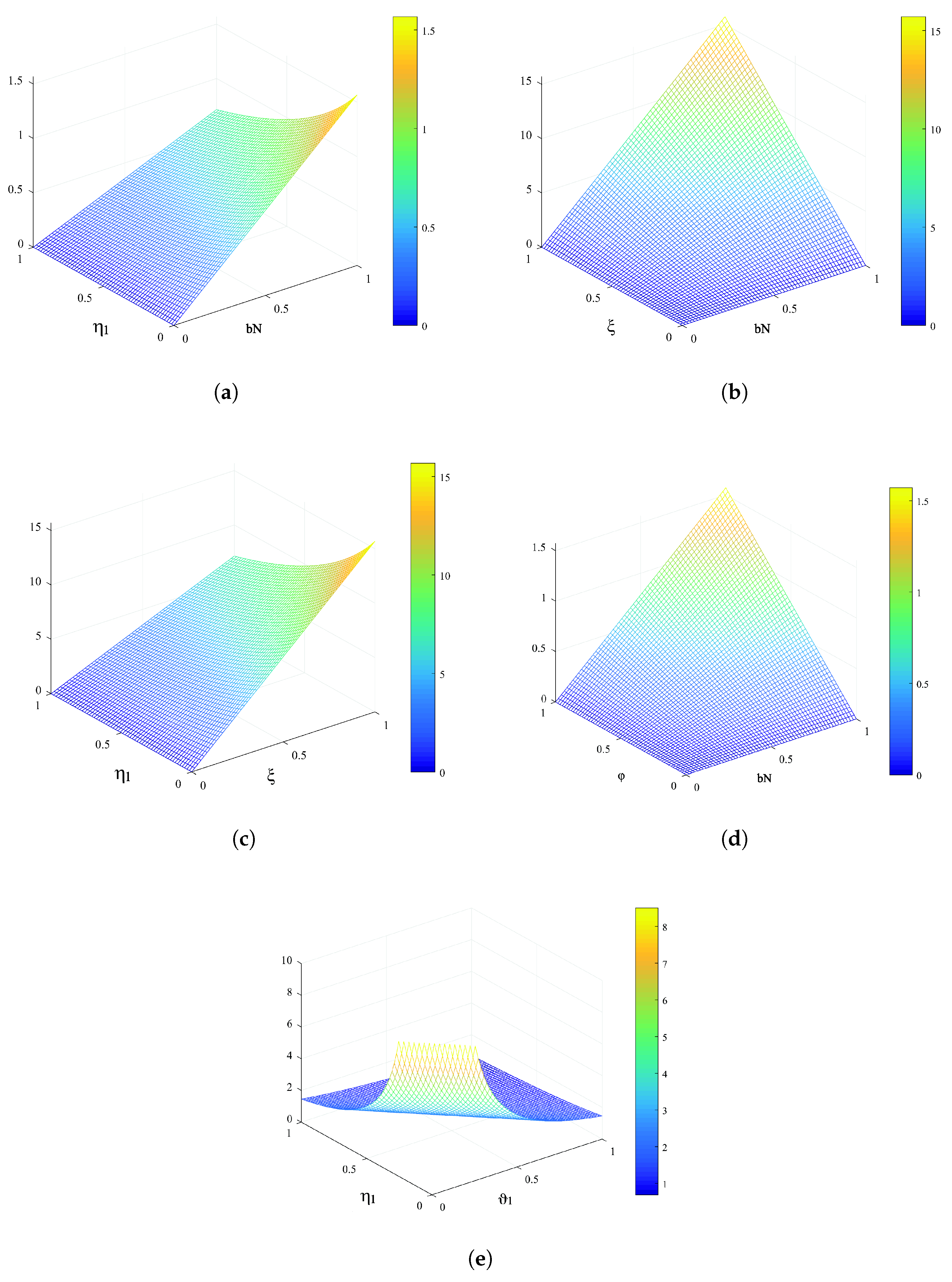
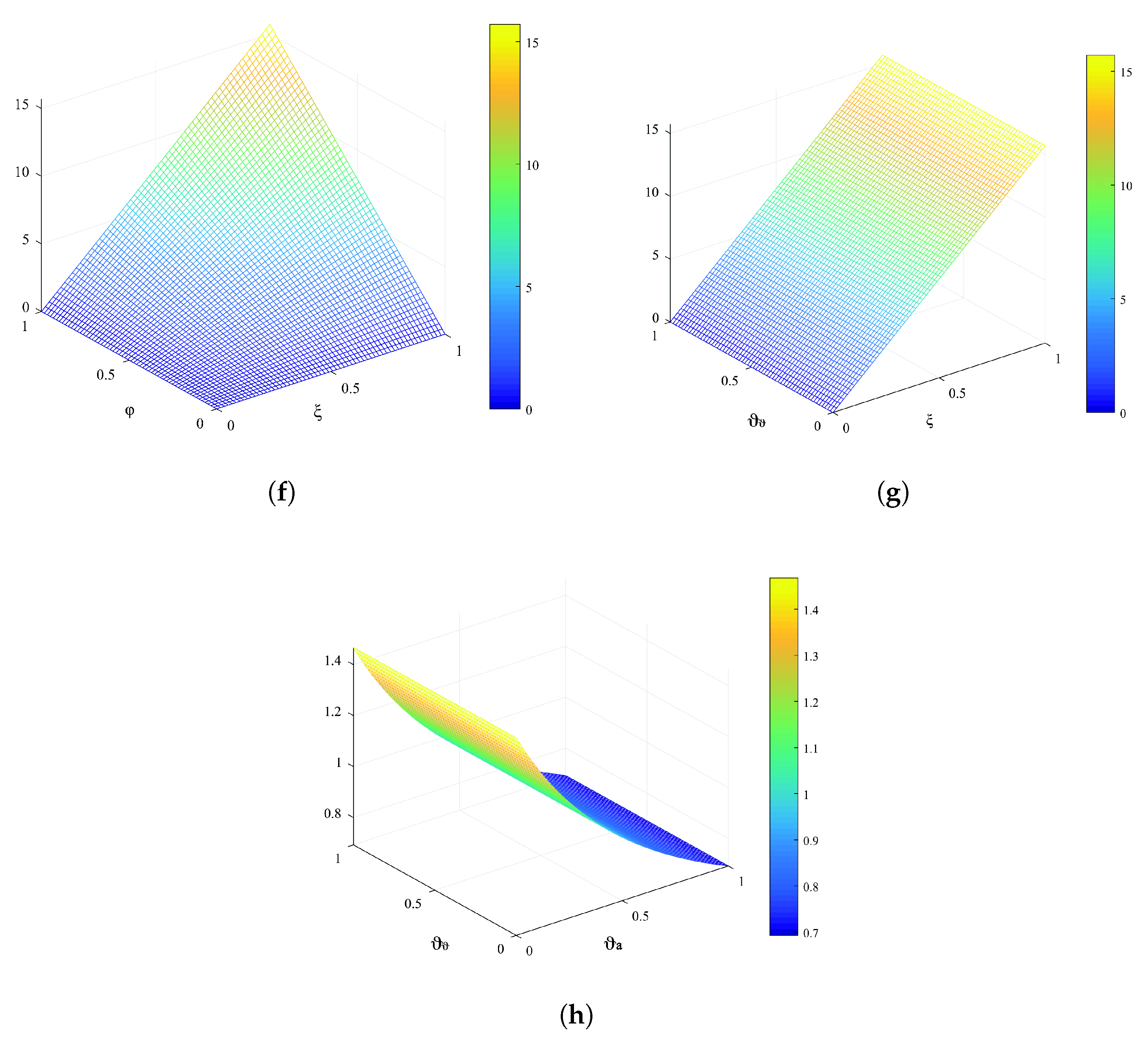
Analysis of Sensitivity

Here, we conduct a sensitivity analysis of some of the parameters used in the model. This technique helps us to identify the parameters that have a significant effect on the basic reproduction number (See Table 1 and Figure 1). We use the approach as described by Chintis [41] to calculate the sensitivity index of R 0 . Specifically, the sensitivity index Δ h R 0 of a parameter h is presented by the formula Δ h R 0 = R 0 k h R 0 .

4. Equilibria Points

The aforementioned system (1) has two possible equilibria: one is the disease-free equilibrium (DFE) and second one is the endemic equilibrium (EE). The DFE, denoted by F 0 , is given by F 0 = b N η 0 , 0 , 0 , 0 , 0 , 0 . The EE, denoted by F 1 , is found by setting “ S = S * , E = E * , I = I * , A = A * , H = H * , and R = R * , and the LHS of the resulting system to zero”. We obtain the following expression after simplification, S * , E * , I * , A * , H * , and R * at the EE.
S * = N b N Q 2 φ Q 2 + φ q ϑ a + η 0 N Q 2 , E * = N b N Q 2 + φ q ϑ a + N b N Q 2 φ Q 2 + φ q ϑ a + η 0 N Q 2 , I * = ( χ ξ ) ( N b N Q 2 + ( R 0 1 ) + N b N Q 2 ) Q 3 φ + φ q ϑ a + η 0 N Q 2 , A * = χ ( 1 ξ ) N b N Q 2 2 + φ q ϑ a + N b N Q 2 φ Q 2 + φ q ϑ a + η 0 N Q 3 , H * = ϑ a I * Q 2 , R * = Q 2 I * + Q 1 Q 2 .

4.1. Local Stability

We show the local asymptotic stability (LAS) of the DFE as well as the EE of the system (1) with the help of the following theorem.
Theorem 1. 
If the basic reproductive number R 0 is less than 1, the DFE point is LAS.
Proof. 
To show the local stability of the system, about the point DFE, the Jacobian matrix for the said system (1) is
J 0 = η 0 0 φ S 0 N 0 φ q S 0 N 0 0 ( χ + η 0 ) φ S 0 N 0 φ q S 0 N 0 0 χ ξ Q 3 0 0 0 0 χ ( 1 ξ ) 0 η 2 0 0 0 0 ϑ a 0 Q 2 0 0 0 ϑ 1 0 ϑ ϑ η 0 .
By conducting a row operation, reducing the matrix to echelon form, the following Jacobian matrix is obtained
η 0 0 φ S 0 N 0 φ q S 0 N 0 0 ( χ + η 0 ) φ S 0 N 0 φ q S 0 N 0 0 0 A φ q S 0 χ ξ N 0 φ q S 0 χ ξ N 0 0 0 B φ q S 0 χ N 0 0 0 0 0 C 0 0 0 0 0 0 D ,
A = Q 3 Q 2 ( χ + η 0 ) φ S 0 χ ξ N , B = ( η 0 + η 2 ) ( χ + η 0 ) Q 1 φ S 0 χ ξ N , C = Q 1 Q 2 Q 3 ( S 0 + η 0 ) , D = η 0 Q 3 ( κ + η 0 ) ( φ S 0 χ ξ ) N [ ( 1 R 0 ) ( N ( χ + η 0 ) Q 2 Q 3 ) φ q S 0 χ ξ ] .
According to [42], when R 0 < 1 , the matrices A , B , C , and D are all negative, and the eigenvalues have negative real parts. As a result, the DFE is LAS. □
Theorem 2. 
If  R 0  is greater than 1, the EE point is LAS.
Proof. 
Consider the Jacobian of the considered problem (1) at F 1 is,
J 0 = φ I * N φ H * q N η 0 0 φ S * N 0 φ q S * N 0 φ I * N + φ H * q N ( χ + η 0 ) φ S * N 0 φ q S * N 0 0 χ ξ Q 3 0 0 0 0 χ ( 1 ξ ) 0 ( η 0 + η 1 ) 0 0 0 0 ϑ a 0 ( ϑ ϑ + η 0 ) 0 0 0 ϑ 1 0 ϑ ϑ η 0 .
After performing a row operation and simplifying the resulting expressions, we obtain the following Jacobian matrix:
φ I * N φ H * q N η 0 0 φ S * N 0 φ q S * N 0 0 ( χ + η 0 ) ( φ I * N + φ H * q S * N + η 0 ) φ S * N 0 φ q S * N 0 0 0 Z 1 η 2 ξ 0 0 0 0 0 Z 2 Z 3 Z 4 0 0 0 0 Z 5 η 0 ϑ ϑ 0 0 0 0 0 Z 6 ,
where
Z 1 = ξ Q 3 , Z 2 = η 2 ( κ + η 0 ) ( φ I * + φ q H * + η 0 ) ϑ 1 , Z 3 = ϑ ϑ φ S * η 0 χ ξ , Z 4 = η 0 φ S * χ ( 1 ξ ) , Z 5 = Q 2 ϑ 1 ϑ a ϑ ϑ , Z 6 = η 0 Q 3 ( η 2 ( χ + η 0 ) ( φ I * + φ q H * + η 0 ) ϑ 1 ( R 0 1 ) × [ ( χ + η 0 ) Q 3 ] ( φ S * η 0 φ ( η 2 ξ ϑ I ) ( ϑ ϑ + η 0 ) ϑ 1 + ϑ a + Q 3 ( η 0 ξ Q 3 ( η 2 ( χ + η 0 ) ) ( φ I * + φ q H * + η 0 ) ϑ 1 + ( ϑ ϑ φ S * η 0 χ ξ ) η 2 ξ ϑ 1 . .
The eigenvalues are given by
ζ 1 = φ I * N φ H * q N η 0 < 0 , ζ 2 = ( χ + η 0 ) ( φ I * N + φ H * q S * N + η 0 ) < 0 , ζ 3 = ξ ( ϑ a + ϑ 1 + η 0 + η 1 ) = Z 1 < 0 , ζ 4 = η 2 ( κ + η 0 ) ( φ I * + φ q H * + η 0 ) ϑ 1 = Z 2 , < 0 , ζ 5 = ( ϑ ϑ + η 0 ) ϑ 1 ϑ a ϑ ϑ = Z 5 < 0 , ζ 6 = Z 6 < 0 . .
As per the findings reported in [43], when R 0 > 1 , all of the eigenvalues have nonpositive real parts, which indicates that the EE point is LAS. □

4.2. Analysis of Global Stability

The next theorem presents that the said system is globally asymptotically stable (GAS) for the DFE and EE point.
Theorem 3. 
The DFE of the system is GAS for R 0 < 1 , otherwise unstable.
Proof. 
We define the Lyapunov function as follows:
U ( t ) = k 1 ( S S 0 ) + k 2 E + k 3 I + k 4 A + k 5 H .
We differentiate Equation (9) and obtain:
U ( t ) = k 1 S + k 2 E + k 3 I + k 4 A + k 5 H .
Using model (1), we obtain
U ( t ) = k 1 [ b N φ I S N φ q H S N η 0 S ] + k 2 [ φ I S N + φ q H S N ( χ + η 0 ) E ] + k 3 [ χ ξ E ( ϑ a + ϑ 1 ) I ( η 0 + η 1 ) I ] + k 4 [ χ ( 1 ξ ) E ( η 0 + η 2 ) A ] + k 5 [ ϑ a I ϑ ϑ H η 0 H ] .
If we choose the positive parameter values k 1 = k 2 = k 4 = ξ , k 3 = 1 , and k 5 = q φ ρ , and simplify, we obtain:
U ( t ) = ξ η 0 ( S S 0 ) 2 φ q H S N Q 1 ξ η 0 E ( η 0 + η 2 ) A Q 3 [ 1 R 0 ] Q 2 Q 3 ( κ + η 0 ) Q 2 2 H .
where
S 0 = b N η 0 ,
Let U ( t ) be a function of time t, and let S and R 0 be constants. If S > S 0 and R 0 < 1 , then U ( t ) is negative. If S = S 0 , then U ( t ) = 0 . According to the LaSalle invariance principle [44,45], if E = I = A = H = 0 , then the set of initial conditions for which U ( t ) approaches zero as t approaches infinity is an invariant set.
Therefore, the DFE F 0 is GAS. □
Theorem 4. 
When  R 0 > 1 , the EE point is GAS at  F 1 , and unstable when  R 0 < 1 .
Proof. 
For the GAS of the EE point, we define the Lyapunov function as:
U ( t ) = 1 2 [ p 1 ( S S * ) + p 2 ( E E * ) + p 3 ( I I * ) + p 4 ( A A * ) + p 5 ( H H * ) ] 2 ,
and we introduce the constants p 1 , p 2 , p 3 , p 4 , and p 5 , which will be chosen later. Upon differentiating Equation (11), we obtain:
U ( t ) = [ p 1 ( S S * ) + p 2 ( E E * ) + p 3 ( I I * ) + p 4 ( A A * ) + p 5 ( H H * ) ] [ p 1 ( d s d t ) + p 2 ( d E d t ) + p 3 ( d I d t ) + p 4 ( d A d t ) + p 5 ( d H d t ) ] ,
U ( t ) = p 1 ( S S * ) + p 2 ( E E * ) + p 3 ( I I * ) + p 4 ( A A * ) + p 5 ( H H * ) ( p 1 ( b N φ I S N φ q H S N η 0 S ) + p 2 ( φ I S N + φ q H S N ( χ + η 0 ) E + p 3 ( χ ξ E ( ϑ a + ϑ 1 ) I ( η 0 + η 1 ) I ) + p 4 ( χ ( 1 ξ ) E ( η 0 + η 2 ) A + p 5 ( ϑ a I ϑ ϑ H η 0 H ) .
After some calculation, we obtain, and utilizing the values of p 1 , p 5 , we obtain
U ( t ) = ( φ S * ) N ( S S * ) ( R 0 1 ) Q 1 Q 2 φ q H * S * N [ E + I + A ] ( ϑ a I ϑ ϑ ) Q 2 Q 3 2 H *
For S = S * and ( ϑ a > ϑ ϑ ) for R 0 is greater than 1; thus, the proof is finished. □

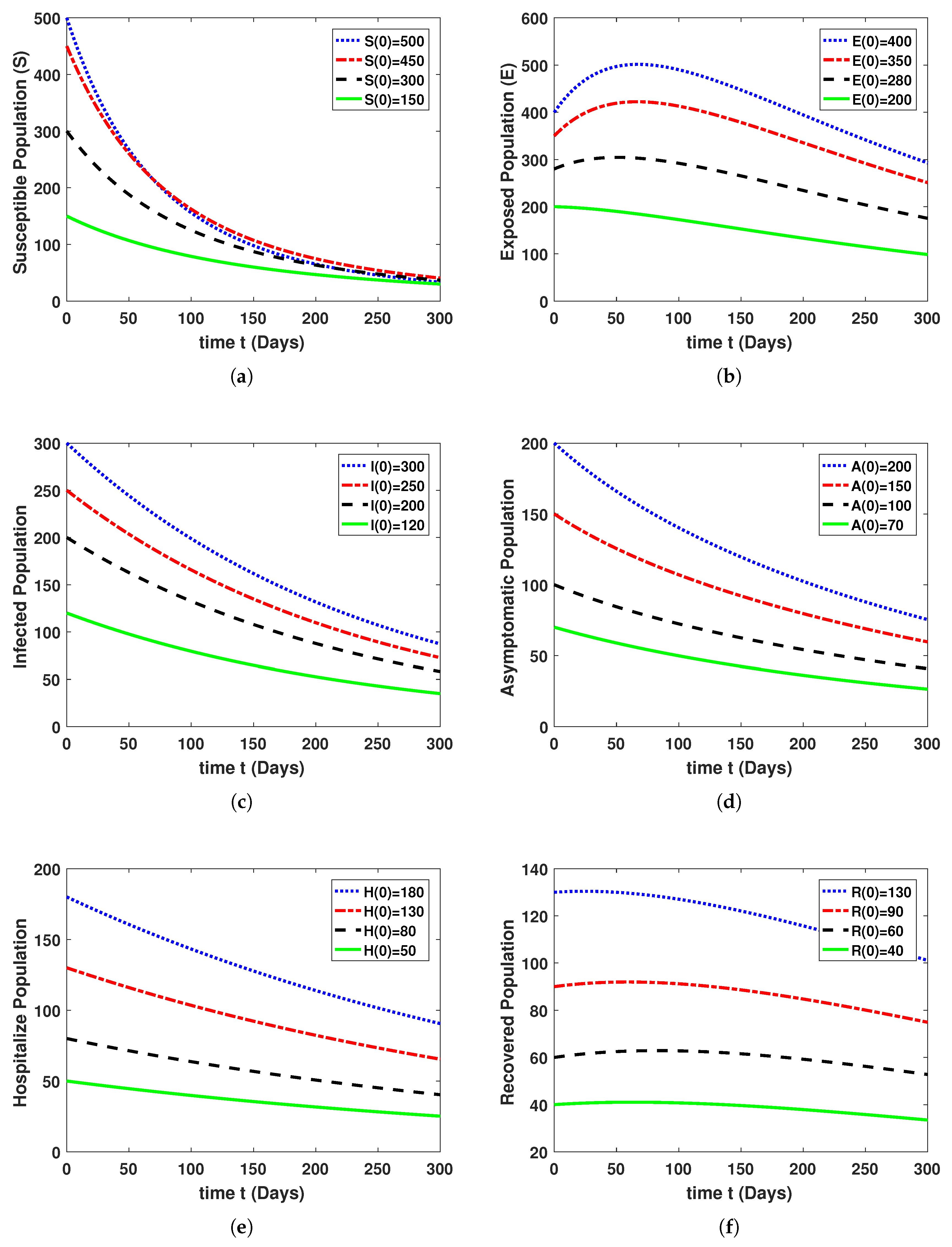
5. Results and Discussion

In this context, we substantiate our analytical discoveries through the application of the fourth-order Runge–Kutta method [46]. We select certain parameters for illustrative purposes, while obtaining others from published data sources [38]. The parameters employed in the simulation are chosen with careful consideration of their biological plausibility. The ensuing set of parameters is utilized for the subsequent analysis. φ = 0.007 ;   q = 0.003 ;   χ = 0.005 ;   ξ = 0.0001 ;   η 0 = 0.0003 ;   η 1 = 0.0001 ;   ξ = 0.002 ;   ϑ 1 = 0.001 ;   ϑ a = 0.000001 ;   ϑ ϑ = 0.0007 ;   and   b N = 0.00004 . To validate the analytical findings of the proposed model concerning the DFE, we employed the aforementioned parameter values. Subsequently, we computed the DFE point’s coordinates and the threshold parameter R 0 as ( 7.98337196 , 0 , 0 , 0 , 0 ) and ( 0.043732 ) , respectively. The simulation outcomes utilizing the aforementioned parameters are depicted in Figure 2 and Figure 3, thereby substantiating the analytical conclusions outlined in the theorem. To corroborate this, we employed the linear stability analysis technique and introduced perturbations to the initial compartmental population values. Remarkably, these perturbed values consistently converged to the DFE, underscoring its robustness against varying initial conditions, S ( 0 ) = 1000 , E ( 0 ) = 800 , I ( 0 ) = 600 , A ( 0 ) = 500 , H ( 0 ) = 400 , and R ( 0 ) = 300 . Drawing from the theoretical interpretation of the data, a definitive conclusion can be drawn: when the value of R 0 is below 1, the disease transmission will inevitably diminish over time. This is evidenced by the convergence of every solution curve to a stable position, as depicted in the corresponding plots.
S i + 1 S i l = b N φ I i S i + 1 N φ q H i S i + 1 N η 0 S i + 1 , E i + 1 E i l = φ I i S i + 1 N + φ q H i S i + 1 N ( χ + η 0 ) E i + 1 , I i + 1 I i l = χ ξ E i + 1 ( ϑ a + ϑ 1 ) I i + 1 ( η 0 + η 1 ) I i + 1 , A i + 1 A i l = χ ( 1 ξ ) E i + 1 ( η 0 + η 2 ) A i + 1 , H i + 1 H i l = ϑ a I i + 1 ϑ ϑ H i + 1 η 0 H i + 1 , R i + 1 R i l = ϑ 1 I i + 1 + ϑ ϑ H i + 1 η 0 R i + 1 .

Used Algorithm

Step 1: ( S 0 , E 0 , I 0 , A 0 , H 0 , R 0 = 0 ) .
Step 2: Let i = 1 , 2 n 1 .
S i + 1 = N l b φ I i S i + 1 + φ q H i S i + 1 l + η 0 l N + S i + 1 φ I i S i + 1 + φ q H i S i + 1 l + η 0 l N , E i + 1 = l φ I i S i + 1 N ( 1 + l ( χ + η 0 ) ) + l φ q H i S i + 1 N ( 1 + l ( χ + η 0 ) ) + E i + 1 ( 1 + l ( χ + η 0 ) ) , I i + 1 = l χ ξ E i + 1 ( 1 + l ( ϑ a + ϑ 1 ) + ( η 0 + η 1 ) l ) + I i + 1 1 + l ( ϑ a + ϑ 1 ) + ( η 0 + η 1 ) l , A i + 1 = l χ ( 1 ξ ) E i + 1 1 + ( η 0 + η 2 ) l + A i + 1 1 + ( η 0 + η 2 ) l , H i + 1 = l ϑ a I i + 1 1 + η 0 l + ϑ ϑ l + H i + 1 1 + ϑ ϑ + η 0 l , R i + 1 = l ϑ 1 I i + 1 1 + η 0 l + l ϑ ϑ H i + 1 1 + η 0 l + R i + 1 1 + η 0 l .
Step 3: Let i = 1 , 2 , 3 , , n 1 , by letting “ S * ( t i ) = S * ,   E * ( t i ) = E * ,   I * ( t i ) = I * ,   A * ( t i ) = A * ,   H * ( t i ) = H * , R * ( t i ) = R * .”
Subsequently, we proceed to explore the system’s dynamics around the EE by assuming an alternate set of parameters: φ = 0.17 , q = 0.03 , χ = 0.05 , ξ = 0.01 , η 0 = 0.03 , η 1 = 0.031 , ξ = 0.052 , ϑ 1 = 0.041 , ϑ a = 0.000001 , ϑ ϑ = 0.0007 , and b N = 0.004 . Using these parameter values acquired earlier, we calculate the endemic equilibrium points and the associated R 0 for the model (1). When R 0 > 1 , the endemic equilibrium point is determined to be ( 40.76549 , 110.908700 , 70.45321 ,   85.934214 , 85.7659321 , 120.7659321 ) , with a calculated value of R 0 = 7.13587 . Assuming the same initial population sizes for the compartments as in the previous analysis, the graphical results indicate that the populations of susceptible, exposed, infected asymptomatic, hospitalized, and recovered individuals initially undergo fluctuations before eventually stabilizing at their respective equilibrium values. For the parameter values employed in this study, the equilibrium point is ( 24.76549 , 99.908700 , 22.45321 , 90.934214 , 85.7659321 , 120.7659321 ) .

6. Analysis of Optimal Control

Here, we aim to establish an effective control strategy to prevent the spread of MERS in the population. Optimal control theory is a powerful mathematical technique that can be applied to design control schemes for a variety of infectious diseases. To achieve this, we apply optimal control theory, as described in previous works [46,47,48,49], to establish an appropriate control strategy. Our objective in this study is to reduce the prevalence of MERS in the populace by increasing the number of persons who recover from the disease, denoted as R , and decreasing the number of individuals who are infectious, denoted as I , and hospitalized, denoted as H , by implementing time-dependent control variables such as treatment v 1 ( t ) and care v 2 ( t ) . In model ( 1 ) , we take six state variables S , E , I , A , H , and R . Now, for the control problem, we take the two control variables, that is treatment v 1 ( t ) and care v 2 ( t ) . Hence, we have the successive optimal control problem to reduce the objective functional
J ( v 1 , v 2 ) = 0 T [ c 1 I ( t ) + c 2 H ( t ) + 1 2 ( c 3 v 1 2 ( t ) + c 4 v 2 2 ( t ) ] d t
subject to
S ˙ ( t ) = b N φ I S N φ q H S N η 0 S , E ˙ ( t ) = φ I S N + φ q H S N ( χ + η 0 ) E , I ˙ ( t ) = χ ξ E ( ϑ a + ϑ 1 ) I ( η 0 + η 1 ) v 1 I , A ˙ ( t ) = χ ( 1 ξ ) E ( η 0 + η 2 ) A , H ˙ ( t ) = ϑ a I ϑ ϑ H η 0 H v 2 H , R ˙ ( t ) = ϑ 1 I + ϑ ϑ H η 0 R + v 1 I + v 2 H ,
with initial conditions
S ( 0 ) 0 , E ( 0 ) 0 , I ( 0 ) 0 , A ( 0 ) 0 , H ( 0 ) 0 , R ( 0 ) 0 .
Equation (12) includes weight constants c 1 , c 2 , c 3 , and c 4 that correspond to the relative importance of infected people I and hospitalized individual H in the objective function. The parameters 1 2 c 3 v 1 2 and 1 2 c 4 v 2 2 represent the costs associated with self-care and treatment. The primary objective is to evaluate the control function to achieve a specific goal.
J ( v 1 * , v 2 * ) = m i n { J ( v 1 , v 2 ) , v 1 , v 2 U }
dependent on control system (13), where U in Equation (14) is known as the control set and is presented as,
U = { ( v 1 , v 2 ) / v i ( t ) is Lebesgue measurable on [ 0 , 1 ] , 0 v i ( t ) 1 , i = 1 , 2 } .
Before proceeding, it is important to establish the existence of control variables. According to Kamien and Aldila’s study [47], a solution for a state system can be found when the controls are bounded and Lebesgue measurable, in addition to satisfying the initial conditions. Thus, we can suppose that the considered control model can be formulated in the manner presented below.
d ϕ d t = A ϕ + B ϕ .
From the above equation ϕ = ( S , E , I , A , H , R ) , where A ( ϕ ) and B ( ϕ ) denote the linear and nonlinear bounded coefficient ∋
J 0 = η 0 0 0 0 0 0 0 ( χ + η 0 ) 0 0 0 0 0 χ ξ Q 3 0 0 0 0 χ ( 1 ξ ) 0 η 2 0 0 0 0 ϑ a 0 Q 2 0 0 0 ϑ 1 0 ϑ ϑ η 0 .
B ( ϕ ) = b N φ I S N φ q H S N φ I S N + φ q H S N 0 0 0 0 .
Letting L ( ϕ ) = A ϕ + F ϕ ,
| F ( ϕ 1 ) F ( ϕ 2 ) | m 1 | S 1 S 2 | + m 2 | E 1 E 2 | + m 3 | I 1 I 2 | + m 4 | A 1 A 2 | + m 5 | H 1 H 2 | + m 6 | R 1 R 2 | N | S 1 S 2 | + | E 1 E 2 | + | I 1 I 2 | + | A 1 A 2 | + | H 1 H 2 | + | R 1 R 2 | .
Here, N = max ( m 1 , m 2 , m 3 , m 4 , m 5 , m 6 ) is a constant that is independent of the state variables in the aforementioned system. We also express
| L ( ϕ 1 ) L ( ϕ 2 ) | M | ( ϕ 1 ) ( ϕ 2 ) | .
The solution for (13) exists due to the nonnegativity of the model state variables S , E , I , A , H , and R . Furthermore, it has been shown that the function L is Lipschitz uniformly continuous, and where M = ( N , K ) < . Based on the properties mentioned earlier, we present the following theorem to establish the existence of a solution for model (1), which we then proceed to prove.
Theorem 5. 
For the control problem in Equations (12) and (13) there exists an optimal control as v * = ( v 1 * , v 2 * ) U .
Proof. 
It is evident that the control and state variables in system (1) are positive. Additionally, the control variables set U is a closed and convex set, as mentioned in the problem statement. Furthermore, the control system is bounded, implying the compactness of the system. The integral in the objective function of the optimization problem, given by c 1 I + c 2 H + 1 2 ( c 3 v 1 2 ( t ) + c 4 v 2 2 ( t ) ) , is also convex w.r.t the control set U . This convexity guarantees the existence results for optimal control for the optimal control variables ( v 1 * , v 2 * ) . □

6.1. Methods

Next to show the optimal solution to the control model (12) and (13), we can apply the Lagrangian and Hamiltonian methods, described in the equation below
L ( I , H , v 1 , v 2 ) = c 1 I + c 2 H + 1 2 ( c 3 v 1 2 ( t ) + c 4 v 2 2 ( t ) .
To describe the Hamiltonian ( H ), by utilizing the notation ϑ = ( ϑ 1 , ϑ 2 , ϑ 3 , ϑ 4 , ϑ 5 , ϑ 6 ) and y = ( y 1 , y 2 , y 3 , y 4 , y 5 , y 6 ) , thus
H ( x , v , ϑ ) = L ( x , v ) + ϑ Z ( x , v ) ,
where
Z 1 = b N φ I S N φ q H S N η 0 S , Z 2 = φ I S N + φ q H S N ( χ + η 0 ) E , Z 3 = χ ξ E ( ϑ a + ϑ 1 ) I ( η 0 + η 1 ) v 1 ( t ) I ( t ) , Z 4 = χ ( 1 ξ ) E ( η 0 + η 2 ) A , Z 5 = ϑ a I ϑ ϑ H η 0 H v 2 ( t ) H ( t ) , Z 6 = ϑ 1 I + ϑ ϑ H η 0 R + v 1 ( t ) I ( t ) + v 2 ( t ) H ( t ) ,
Thus we apply the Pontryagin Maximum Principle [50,51] to the Hamiltonian in order to determine the optimal solution. According to this principle, if ( x * , v * ) is an optimal solution, then there must exist a function ϑ ∋:
d x d t = H ϑ , 0 = H u , ϑ ( t ) = H x .
H ( t , x * , v * , ϑ ) x = m a x v 1 , v 2 , v 3 , v 4 [ 0 , 1 ] H ( x * ( t ) , v 1 , v 2 ϑ ( t ) ) ;
with
ϑ ( t f ) = 0 ,
The principles outlined in Equation (19) are utilized to determine the adjoint system (adjoint variables) and optimal control variables. Based on these principles, the following result can be obtained.
Theorem 6. 
Suppose S * , E * , I * , A * , H * , and R * represent the optimal state solutions for the system, obtained using the combined optimal control variables ( v 1 * , v 2 * ) that were derived through the numerical solution of the optimality system. The optimal control problem is defined by the objective function (12) and the control system (13). Thenadjoint variables ϑ 1 ( t ) , ϑ 2 ( t ) , ϑ 3 ( t ) , and ϑ 4 ( t ) , ϑ 5 ( t ) , ϑ 6 ( t ) satisfy
ϑ 1 ( t ) = A 1 + ( ϑ 2 ϑ 1 ) φ I * + ( ϑ 2 ϑ 1 ) φ q H * η 0 ϑ 1 , ϑ 2 ( t ) = A 2 + ( ϑ 4 ϑ 2 ) φ N * + ( χ + η 0 ) ϑ 2 ϑ 1 v 1 * ϑ 3 ξ , ϑ 3 ( t ) = A 3 + ( ϑ 2 ϑ 1 ) φ S * + ( ϑ 5 ϑ 3 ) ϑ a + ( ϑ 6 ϑ 3 ) ϑ 1 + ( ϑ 6 ϑ 3 ) v 1 ( t ) v 1 ϑ 3 , ϑ 4 ( t ) = A 4 + ( v 2 u 0 ) ϑ 4 , ϑ 5 ( t ) = A 5 ( ϑ 2 ϑ 1 ) φ q S * + ( ϑ 6 ϑ 5 ) ϑ ϑ ( u 0 + v 2 ) ϑ 5 , ϑ 6 ( t ) = A 6 + u 0 ϑ 6 ,
with boundary conditions.
Additionally, the optimal control parameters v 1 ( t ) and v 2 ( t ) are obtained through numerical solutions of the optimality problem and are presented below.
v 1 * ( t ) = m a x { m i n { ( ϑ 6 ϑ 3 ) I * B 1 , 1 } , 0 } ,
v 2 * ( t ) = m a x { m i n { ( ϑ 6 ϑ 5 ) H * B 2 , 1 } , 0 } .
Proof. 
The adjoint problem described by Equation (21) is obtained through the uses of the Pontryagin Maximum Principle given by Equation (19), while the transversal conditions arise from ϑ ( T ) = 0 . The set of optimal functions v 1 * , v 2 is obtained using H u . In the following section, we present numerical solutions to the optimality system in order to provide a clearer understanding for the reader, as opposed to relying solely on analytical results. The optimality problem is expressed by several components, including the control problem (13), the adjoint model (21), the boundary (terminal) conditions, and the optimal control functions. By solving these components numerically, we can gain valuable insights into the behavior of the system and assess its performance. □

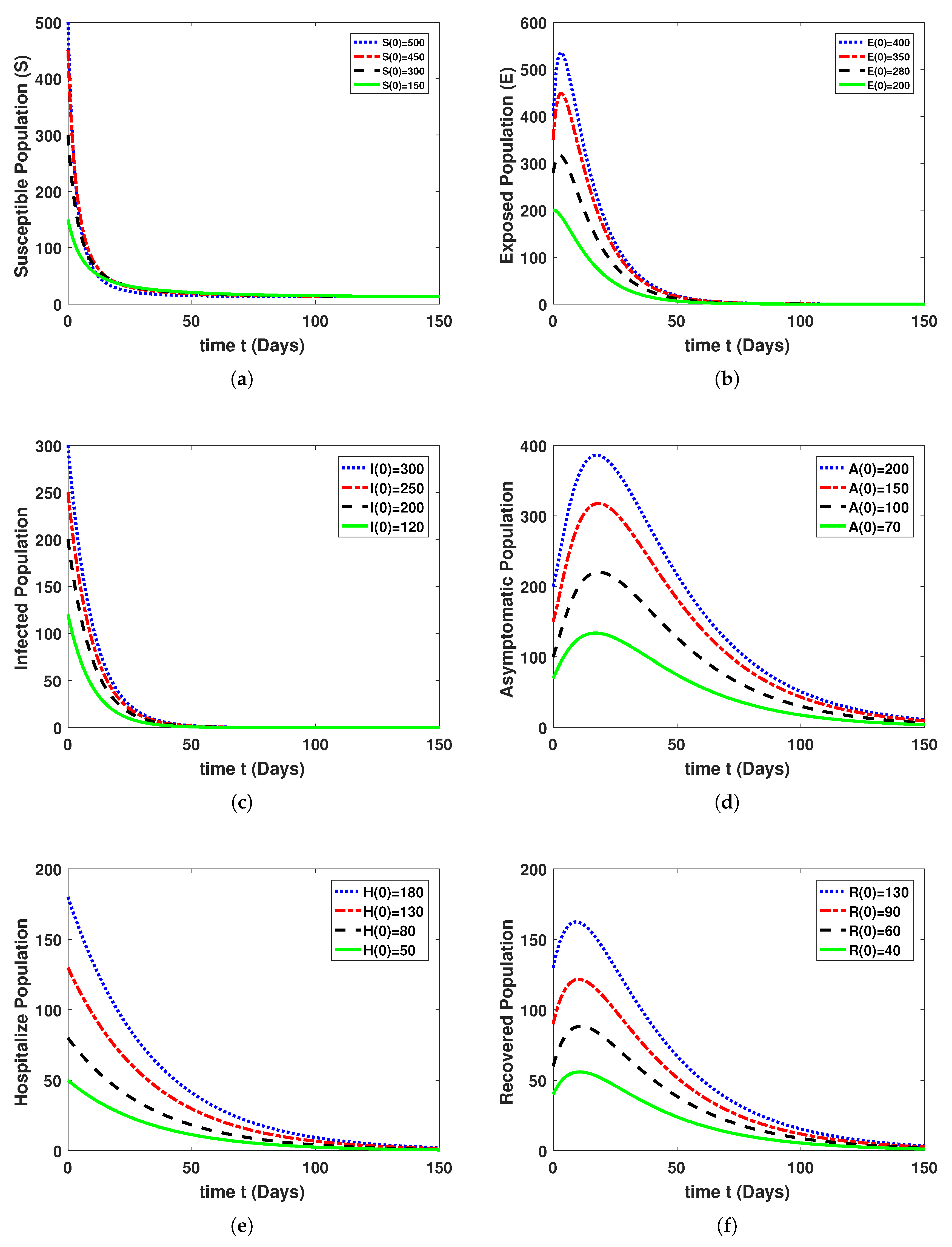
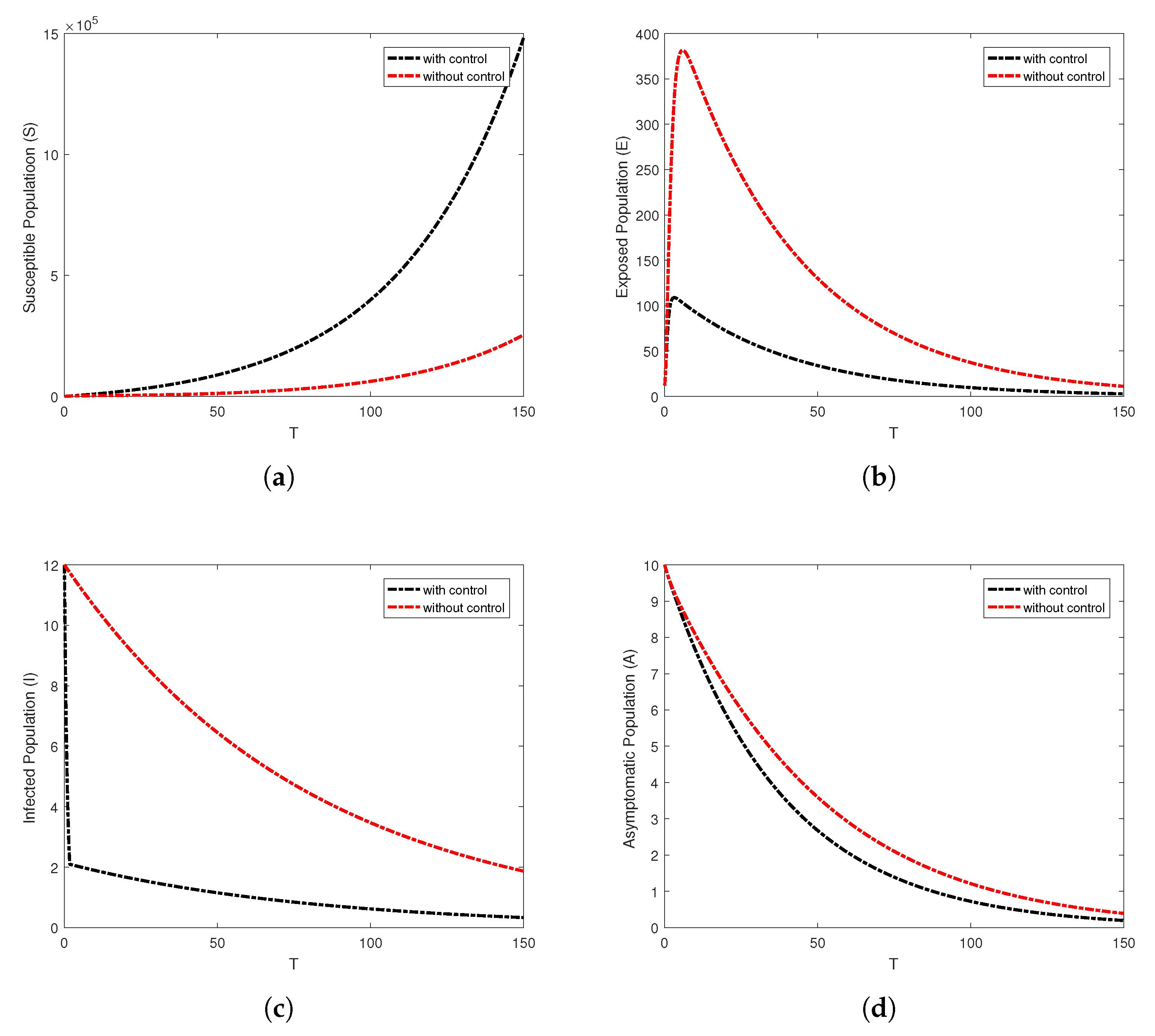
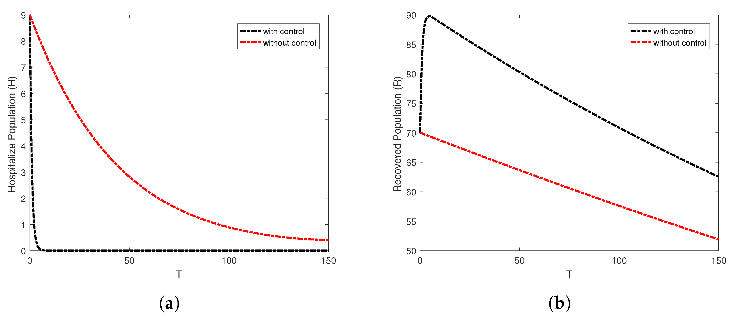
6.2. Results and Discussion for Optimal Control

We utilize the Runge–Kutta method of order four to solve the optimal control system (13), in order to investigate the effects of self-care and treatment. To find the solution of the state system (12) with initial conditions in the time interval [0, 50], we employ the forward Runge–Kutta procedure. Similarly, the backward Runge–Kutta technique is used to solve the adjoint system (21) in the same interval with the assistance of the transversality condition. Below are the parameters that we used for the simulation: b N = 0.0071 ;   φ = 0.00041 ;   q = 0.0000123 ;   χ = 0.0000123 ;   ξ = 0.0000123 ;   ϑ 1 = 0.003907997 ;   ϑ a = 0.98 ;   ϑ ϑ = 0.0000404720925 ;   q = 0.017816 ;   ρ = 0.00007 ; a n d   η 0 = 0.00997 . The weight constants c 1 , c 2 , c 3 , and c 4 were chosen based on biological feasibility. Specifically, we set c 1 = 0.6610000 ,   c 2 = 0.54450 ,   c 3 = 0.0090030 ,   c 4 = 0.44440 . The results obtained from the simulations are presented in Figure 4 and Figure 5.
Figure 4 and Figure 5 show the variations in the number of all compartments with and without control measures implemented.

7. Conclusions

The objective of this study is to developed a more realistic mathematical model that captures the transmission dynamics of the MERS-CoV. This is accomplished by introducing new parameters for the birth and death rates in the host populace. The threshold number R 0 is a measure used to estimate the potential spread of a disease within a populace, and it can be calculated from a model to quantify the transmissibility of MERS-CoV. The model is analyzed using stability theory to identify conditions for local and global stability, and the most sensitive parameter is determined through a sensitivity analysis of R 0 . An optimal control problem is formulated with the goal of minimizing the number of infected persons and maximizing the number of recoveries in the population. The effectiveness of the approach is verified through numerical simulations, which demonstrate the stability of the results.

Author Contributions

Conceptualization, B.F., M.Y. and M.u.R.; methodology, A.A. and S.A.; software, B.F.; validation, M.Y. and M.u.R.; formal analysis, M.Y.; investigation, A.A.; resources, S.A.; data curation, B.F.; writing—original draft preparation, B.F., M.Y. and M.u.R.; writing—review and editing, M.Y. and A.A.; supervision, S.A. All authors have read and agreed to the published version of the manuscript.

Funding

This research received no external funding.

Data Availability Statement

Not applicable.

Acknowledgments

The researchers would like to acknowledge Deanship of Scientific Research, Taif University for funding this work.

Conflicts of Interest

The authors declare no conflict of interest.

References

  1. AlTawfiq, J.A.; Hinedi, K.; Ghandour, J. Middle East respiratory syndrome coronavirus: A case-control study of hospitalized patients. Clin. Infect. Dis. 2014, 59, 160–165. [Google Scholar] [CrossRef] [PubMed]
  2. Azhar, E.I.; Kafrawy, E.I.; Hassan, S.A.; Al-Saeed, A.M.; Hashem, M.S.; Madani, A.M. Evidence for camel to human transmission of MERS coronavirus. N. Engl. J. Med. 2014, 370, 2499–2505. [Google Scholar] [CrossRef] [PubMed]
  3. Arabi, Y.M.; Arifi, A.A.; Balkhy, H.H. Clinical course and outcomes of critically ill patients with Middle East respiratory syndrome coronavirus infection. Ann. Intern. Med. 2014, 160, 389–397. [Google Scholar] [CrossRef] [PubMed]
  4. Madani, T.A.; Azhar, E.I.; Hashem, A.M. Evidence for camel-to-human transmission of MERS coronavirus. N. Engl. J. Med. 2014, 371, 1360. [Google Scholar] [PubMed]
  5. Breban, R.; Riou, J.; Fontanent, A. Interhuman transmissibility of Middle East respiratory coronavirus: Estimation of pandemic risk. Lancet 2013, 382, 694–699. [Google Scholar] [CrossRef]
  6. Fisman, D.N.; Ashleigh, R.T. The epidemiology of MERS-CoV. Lancet Infect. Dis. 2014, 14, 6–7. [Google Scholar] [CrossRef]
  7. Zhong, N.S.; Zheng, B.J.; Li, Y.M.; Poon, L.L.M.; Xie, Z.H.; Chan, K.H.; Li, P.H.; Tan, S.Y.; Chang, Q.; Xie, J.P.; et al. Epidemiology and cause of severe acute respiratory syndrome (SARS) in Guangdong, People’s Republic of China, in February, 2003. Lancet 2003, 362, 1353–1358. [Google Scholar] [CrossRef]
  8. Ksiazek, T.G.; Erdman, D.; Goldsmith, C.S.; Zaki, S.R.; Peret, T.; Emery, S.; Tong, S.; Urbani, C.; Comer, J.A.; Lim, W.; et al. A novel coronavirus associated with severe acute respiratory syndrome. N. Engl. J. Med. 2003, 348, 1953–1966. [Google Scholar] [CrossRef]
  9. Zaki, A.M.; Van Boheemen, S.; Bestebroer, T.M.; Osterhaus, A.D.; Fouchier, R.A. Isolation of a novel coronavirus from a man with pneumonia in Saudi Arabia. N. Engl. J. Med. 2012, 367, 1814–1820. [Google Scholar] [CrossRef]
  10. Ciotti, M.; Ciccozzi, M.; Terrinoni, A.; Jiang, W.C.; Wang, C.B.; Bernardini, S. The COVID-19 pandemic. Crit. Rev. Clin. Lab. Sci. 2020, 57, 365–388. [Google Scholar] [CrossRef]
  11. Mandal, M.; Jana, S.; Nandi, S.K.; Khatua, A.; Adak, S.; Kar, T.K. A model based study on the dynamics of COVID-19: Prediction and control. Chaos Solitons Fractals 2020, 136, 109889. [Google Scholar] [CrossRef] [PubMed]
  12. Atede, A.O.; Omame, A.; Inyama, S.C. A fractional order vaccination model for COVID-19 incorporating environmental transmission: A case study using Nigerian data. Bull. Biomath. 2023, 1, 78–110. [Google Scholar] [CrossRef]
  13. Shen, Z.H.; Chu, Y.M.; Khan, M.A.; Muhammad, S.; Al-Hartomy, O.A.; Higazy, M. Mathematical modeling and optimal control of the COVID-19 dynamics. Results Phys. 2021, 31, 105028. [Google Scholar] [CrossRef] [PubMed]
  14. Alqarni, M.S.; Alghamdi, M.; Muhammad, T.; Alshomrani, A.S.; Khan, M.A. Mathematical modeling for novel coronavirus (COVID-19) and control. Numer. Methods Partial. Differ. Equ. 2022, 38, 760–776. [Google Scholar] [CrossRef]
  15. Tsay, C.; Lejarza, F.; Stadtherr, M.A.; Baldea, M. Modeling, state estimation, and optimal control for the US COVID-19 outbreak. Sci. Rep. 2020, 10, 10711. [Google Scholar] [CrossRef]
  16. Libotte, G.B.; Lobato, F.S.; Platt, G.M.; Neto, A.J.S. Determination of an optimal control strategy for vaccine administration in COVID-19 pandemic treatment. Comput. Methods Programs Biomed. 2020, 196, 105664. [Google Scholar] [CrossRef]
  17. Ullah, I.; Ahmad, S.; Al-Mdallal, Q.; Khan, Z.A.; Khan, H.; Khan, A. Stability analysis of a dynamical model of tuberculosis with incomplete treatment. Adv. Differ. Equ. 2020, 2020, 499. [Google Scholar] [CrossRef]
  18. Hajji Mohamed, A.; Al-Mdallal, Q. Numerical simulations of a delay model for immune system-tumor interaction. Sultan Qaboos Univ. J. Sci. (SQUJS) 2018, 23, 19–31. [Google Scholar]
  19. Asif, M.; Haider, N.; Al-Mdallal, Q.; Khan, I. A Haar wavelet collocation approach for solving one and two-dimensional second-order linear and nonlinear hyperbolic telegraph equations. Numer. Methods Partial. Differ. Equ. 2020, 36, 1962–1981. [Google Scholar] [CrossRef]
  20. Kermack, W.O.; McKendrick, A.G. Contributions to the mathematical theory of epidemics, part 1. Proc. R. Soc. Edinburgh. Sect. A Math. 1927, 115, 700–721. [Google Scholar]
  21. Cauchemez, S.; Fraser, C.; Van Kerkhove, M.D.; Donnelly, C.A.; Riley, S.; Rambaut, A.; Enouf, V.; van der Werf, S.; Ferguson, N.M. Middle East respiratory syndrome coronavirus: Quantification of the extent of the epidemic, surveillance biases, and transmissibility. Lancet Infect. Dis. 2013, 14, 50–56. [Google Scholar] [CrossRef]
  22. Chowell, G.; Blumberg, S.; Simonsen, L.; Miller, M.A.; Viboud, C. Synthesizing data and models for the spread of MERS-CoV, 2013: Key role of index cases and hospital transmission. Epidemics 2014, 9, 40–51. [Google Scholar] [CrossRef] [PubMed]
  23. Assiri, A.; Al-Tawfiq, J.A.; Al-Rabeeah, A.A.; Al-Rabiah, F.A.; Al-Hajjar, S.; Al-Barrak, A. Epidemiological, demographic, and clinical characteristics of 47 cases of Middle East respiratory syndrome coronavirus disease from Saudi Arabia: A descriptive study. Lancet Infect. Dis. 2013, 13, 752–761. [Google Scholar] [CrossRef] [PubMed]
  24. Li, B.; Eskandari, Z.; Avazzadeh, Z. Dynamical behaviors of an SIR epidemic model with discrete time. Fractal Fract. 2022, 6, 659. [Google Scholar] [CrossRef]
  25. Li, B.; Eskandari, Z. Dynamical analysis of a discrete-time SIR epidemic model. J. Frankl. Inst. 2023, 360, 7989–8007. [Google Scholar] [CrossRef]
  26. Li, B.; Eskandari, Z.; Avazzadeh, Z. Strong resonance bifurcations for a discrete-time prey–predator model. J. Appl. Math. Comput. 2023, 69, 2421–2438. [Google Scholar] [CrossRef]
  27. Jiang, X.; Li, J.; Li, B.; Yin, W.; Sun, L.; Chen, X. Bifurcation, chaos, and circuit realisation of a new four-dimensional memristor system. Int. J. Nonlinear Sci. Numer. Simul. 2022. [Google Scholar] [CrossRef]
  28. Sabbar, Y. Asymptotic extinction and persistence of a perturbed epidemic model with different intervention measures and standard lévy jumps. Bull. Biomath. 2023, 1, 58–77. [Google Scholar] [CrossRef]
  29. Adoum, A.H.; Haggar, M.S.D.; Ntaganda, J.M. Mathematical modelling of a glucose-insulin system for type 2 diabetic patients in Chad. Math. Model. Numer. Simul. Appl. 2022, 2, 244–251. [Google Scholar] [CrossRef]
  30. Ahmed, I.; Akgül, A.; Jarad, F.; Kumam, P.; Nonlaopon, K. A Caputo-Fabrizio fractional-order cholera model and its sensitivity analysis. Math. Model. Numer. Simul. Appl. 2023, 3, 170–187. [Google Scholar] [CrossRef]
  31. Singh, T.; Vaishali; Adlakha, N. Numerical investigations and simulation of calcium distribution in the alpha-cell. Bull. Biomath. 2023, 1, 40–57. [Google Scholar] [CrossRef]
  32. Odionyenma, U.B.; Ikenna, N.; Bolaji, B. Analysis of a model to control the co-dynamics of Chlamydia and Gonorrhea using Caputo fractional derivative. Math. Model. Numer. Simul. Appl. 2023, 3, 111–140. [Google Scholar] [CrossRef]
  33. Yao, T.-T.; Qian, J.-D.; Zhu, W.-Y.; Wang, Y.; Wang, G.-Q. A systematic review of lopinavir therapy for SARS coronavirus and MERS coronavirus—A possible reference for coronavirus disease-19 treatment option. J. Med. Virol. 2020, 92, 556–563. [Google Scholar] [CrossRef] [PubMed]
  34. Fatima, B.; Yavuz, M.; Rahman, M.u.; Al-Duais, F.S. Modeling the epidemic trend of middle eastern respiratory syndrome coronavirus with optimal control. Math. Biosci. Eng. 2023, 20, 11847–11874. [Google Scholar] [CrossRef]
  35. Afshar, Z.M.; Ebrahimpour, S.; Javanian, M.; Koppolu, V.; Vasigala, V.K.R.; Hasanpour, A.H.; Babazadeh, A. Coronavirus disease 2019 (COVID-19), MERS and SARS: Similarity and difference. J. Acute Dis. 2020, 9, 194–199. [Google Scholar]
  36. Ahmad, S.; Dong, Q.; Rahman, M.u. Dynamics of a fractional-order COVID-19 model under the nonsingular kernel of Caputo-Fabrizio operator. Math. Model. Numer. Simul. Appl. 2022, 2, 228–243. [Google Scholar] [CrossRef]
  37. ur Rahman, M.; Arfan, M.; Baleanu, D. Piecewise fractional analysis of the migration effect in plant-pathogen-herbivore interactions. Bull. Biomath. 2023, 1, 1–23. [Google Scholar] [CrossRef]
  38. Yunhwan, K.; Sunmi, L.; Chaeshin, C.; Seoyun, C.; Saeme, H.; Youngseo, S. The Characteristics of Middle Eastern Respiratory Syndrome Coronavirus Transmission Dynamics in South Korea. Osong Public Health Res. Perspect. 2016, 7, 49–55. [Google Scholar]
  39. Driessch, V.; Watmough, J. Reproduction numbers and sub threshold endemic equilibria for compartmental models of disease transmission. Math. Biosci. 2002, 180, 29–48. [Google Scholar] [CrossRef]
  40. Van Den Driessche, P.; Watmough, J. Mathematical Epidemiology; Springer: Berlin/Heidelberg, Germany, 2008. [Google Scholar]
  41. Chitnis, N.; Cushing, J.M.; Hyman, J.M. Bifurcation analysis of a mathematical model for malaria transmission. SIAM J. Appl. Math. 2006, 67, 24–45. [Google Scholar] [CrossRef]
  42. Khan, T.; Zaman, G.; Chohan, M.I. The transmission dynamic and optimal control of acute and chronic hepatitis B. J. Biol. Dyn. 2017, 11, 172–189. [Google Scholar] [CrossRef]
  43. Zaman, G.; Han Kang, Y.; Jung, I.H. Stability analysis and optimal vaccination of an SIR epidemic model. Biosystems 2008, 93, 240–249. [Google Scholar] [CrossRef] [PubMed]
  44. LaSalle, J.P. The Stability of Dynamical System; SIAM: Philadelphia, PA, USA, 1976. [Google Scholar]
  45. LaSalle, J.P. Stability of nonautonomous system. Nonlinear Anal. 1976, 1, 83–90. [Google Scholar] [CrossRef]
  46. Khan, T.; Ullah, Z.; Ali, N.; Zaman, G. Modeling and control of the hepatitis b virus spreading using an epidemic model. Chaos Solitons Fractals 2019, 124, 1–9. [Google Scholar] [CrossRef]
  47. Kamien, M.; Schwartz, N. Dynamic Optimization, 2nd ed.; North-Holland: Amsterdam, The Netherlands, 1991. [Google Scholar]
  48. Hattaf, K.; Yousfi, N. Optimal control of a delayed HIV infection model with immune response using an efficient numerical method. Int. Sch. Res. Not. 2012, 2012, 215124. [Google Scholar] [CrossRef]
  49. Evirgen, F.; Ozköse, F.; Yavuz, M.; Ozdemir, N. Real data-based optimal control strategies for assessing the impact of the Omicron variant on heart attacks. AIMS Bioeng. 2023, 10, 218–239. [Google Scholar] [CrossRef]
  50. Lashari, A.A.; Zaman, G. Global dynamics of vector-borne diseases with horizontal transmission in host population. Comput. Math. Appl. 2001, 61, 745–754. [Google Scholar] [CrossRef]
  51. Aseev, S.M.; Kryazhimskii, A.V. The Pontryagin maximum principle and optimal economic growth problems. Proc. Steklov Inst. Math. 2007, 257, 1–255. [Google Scholar] [CrossRef]
Figure 1. The graphs display the results of a sensitivity analysis on the basic reproductive number R 0 . (a) R 0 with η 1 , b N ; (b) R 0 with ξ , b N ; (c) R 0 with η 1 , ξ ; (d) R 0 with φ , b N ; (e) R 0 with η 1 , ϑ 1 ; (f) R 0 with φ , ξ ; (g) R 0 with ϑ ϑ , ξ ; (h) R 0 with ϑ ϑ , ϑ a .
Mca 28 00098 g001aMca 28 00098 g001b
Figure 2. The time dynamics of the compartmental populations in model (1) are shown graphically for an initial population value. (a) Class of S ; (b) class of E ; (c) class of I ; (d) class of A ; (e) class of H ; (f) class of R .
Mca 28 00098 g002
Figure 3. The time dynamics of the compartmental populations in model (1) are shown graphically for initial population values. (a) Class of S ; (b) class of E ; (c) class of I ; (d) class of A ; (e) class of H ; (f) class of R .
Mca 28 00098 g003
Figure 4. The visual representations demonstrate the changes in the compartmental population over time, comparing the scenarios with and without control measures implemented. (a) Susceptible populace; (b) exposed populace; (c) infected population; (d) asymptomatic population.
Mca 28 00098 g004
Figure 5. The visual representations demonstrate the changes in the compartmental population over time, comparing the scenarios with and without control measures implemented. (a) Hospitalized population; (b) recovered population.
Mca 28 00098 g005
Table 1. Sensitivity indices of different parameters.
NotationSensitivity ValuesNotationSensitivity Values
χ 0.0384651 ϑ 1 −0.058565
ϑ ϑ −0.00000453 ϑ a −0.93704
η 0 −0.001464128 η 1 −0.041392
φ 0.99999q0.0000476
b N 0.99999 ξ 0.000432
Disclaimer/Publisher’s Note: The statements, opinions and data contained in all publications are solely those of the individual author(s) and contributor(s) and not of MDPI and/or the editor(s). MDPI and/or the editor(s) disclaim responsibility for any injury to people or property resulting from any ideas, methods, instructions or products referred to in the content.

