Preconditioning Technique for an Image Deblurring Problem with the Total Fractional-Order Variation Model

Abstract

Total fractional-order variation (TFOV) in image deblurring problems can reduce/remove the staircase problems observed with the image deblurring technique by using the standard total variation (TV) model. However, the discretization of the Euler–Lagrange equations associated with the TFOV model generates a saddle point system of equations where the coefficient matrix of this system is dense and ill conditioned (it has a huge condition number). The ill-conditioned property leads to slowing of the convergence of any iterative method, such as Krylov subspace methods. One treatment for the slowness property is to apply the preconditioning technique. In this paper, we propose a block triangular preconditioner because we know that using the exact triangular preconditioner leads to a preconditioned matrix with exactly two distinct eigenvalues. This means that we need at most two iterations to converge to the exact solution. However, we cannot use the exact preconditioner because the Shur complement of our system is of the form $S=K^{*}K+\lambda L_{\alpha }$ which is a huge and dense matrix. The first matrix, $K{}^{*}K$, comes from the blurred operator, while the second one is from the TFOV regularization model. To overcome this difficulty, we propose two preconditioners based on the circulant and standard TV matrices. In our algorithm, we use the flexible preconditioned GMRES method for the outer iterations, the preconditioned conjugate gradient (PCG) method for the inner iterations, and the fixed point iteration (FPI) method to handle the nonlinearity. Fast convergence was found in the numerical results by using the proposed preconditioners.

1. Introduction

Although TV regularization is a commonly employed technique in image deblurring problems [1,2,3,4], one significant drawback is the appearance of the “staircase effect”, wherein edges are depicted as a sequence of steps rather than smooth transitions. This phenomenon arises because TV regularization encourages the creation of piecewise constant regions, which leads to the appearance of blocks around edges rather than accurately capturing their continuous nature. As a result, researchers are actively investigating and advancing alternative regularization techniques and algorithms to remove or reduce these “staircase effects” and enhance the overall quality of image deblurring methods. An alternative regularization approach is the TFOV model [5,6,7,8]. TFOV regularization presents a robust method for enhancing image deblurring, offering a combination of benefits such as edge preservation, flexibility, noise resilience, and reduction in staircase effects. Its effectiveness has been substantiated in numerous studies, significantly contributing to the progression of image deblurring techniques. However, when it comes to discretizing the Euler–Lagrange equations of the TFOV-based model, a substantial nonlinear and ill-conditioned system emerges. Efficiently solving such systems poses a considerable challenge for numerical methods, even with the application of potent numerical algorithms like Krylov subspace methods, such as the generalized minimal residual (GMRES) and conjugate gradient (CG). These methods tend to exhibit slow convergence in this context. One potential remedy to address this slow convergence is the use of preconditioning techniques. Preconditioning is a technique used to transform a linear system of the form $Ax=b$ into another system to improve the spectral properties of the system matrix. A preconditioner is a matrix P that is easy to invert and the preconditioned matrix $P^{-1}A$ shows good clustering behavior for the eigenvalues. This is because rapid convergence is often associated with a clustered spectrum of $P^{-1}A$. In the preconditioning technique, we solve $P^{-1}Ax=P^{-1}b$ instead of solving the original $Ax=b$ because the new system $P^{-1}Ax=P^{-1}b$ converges rapidly when we use a suitable preconditioner. To apply the preconditioner matrix P within a Krylov subspace method, we need to compute the multiplication of a matrix by a vector of the form $z=Pr$ at each iteration. Hence, evaluating this product must be cheap. In the literature, several preconditioners are developed in [9] for a special linear system, such as block preconditioners and constraint preconditioners. For diagonal preconditioners, we can refer to Silvester and Wathen [10] and Wathen and Silvester [11]. For the block triangular preconditioners, we can refer to Bramble and Pasciak [12] and [13,14,15,16], as well as the references therein. For constraint preconditioners, see, for example, Axelsson and Neytcheva [17]. Other preconditioners based on Hermitian/skew-Hermitian splitting are studied in [18,19,20]. Recently, several new preconditioners for Krylov subspace methods have been introduced. For example, Cao et al. [21] derived two block triangular Schur complement preconditioners from a splitting of the ($1,1$)-block of the two-by-two block matrix. Chen and Ma [22] proposed a generalized shift-splitting preconditioner for saddle point problems with a symmetric positive definite ($1,1$)-block. Salkuyeh et al. [23] proposed a modified generalized shift-splitting preconditioner where the ($1,1$)-block is symmetric positive definite and the ($2,2$)-block matrix is symmetric positive semidefinite (not zero). Very recently, block diagonal and block triangular splitting preconditioners were studded by Beik et al. [24], and the authors introduced new variants of the splitting preconditioners and obtained new results for the convergence of the associated stationary iterations and new bounds for the eigenvalues of the corresponding preconditioned matrices. Moreover, they considered inexact versions as preconditioners for flexible Krylov subspace methods. A good survey of preconditioning techniques for general linear systems can be found in [9,25,26].

In our paper, we consider the following two-by-two block nonlinear system of equations:

$$\underset{\mathrm{A}}{\underbrace{\left[\begin{array}{cc}{I}_n\hfill & K_h\hfill \\ -K_h^{*}\hfill & \lambda L_h^{\alpha }\left(U_h\right)\hfill \end{array}\right]}}\underset{\mathrm{x}}{\underbrace{\left[\begin{array}{c}{V}_h\hfill \\ U_h\hfill \end{array}\right]}}=\underset{\mathrm{b}}{\underbrace{\left[\begin{array}{c}{Z}_h\hfill \\ 0\hfill \end{array}\right]}}.$$

(1)

This system is obtained by discretizing the Euler-Lagrange equations associated with TFOV in image deblurring problems, and the coefficient matrix of this system has a size of $2n$ by $2n$, where $n:=N^2$ and N is the number of pixels in the image. The coefficient matrix of this system is non-symmetric, ill conditioned, dense, and huge. These properties complicate the development of an efficient numerical algorithm. We know that using direct methods for solving Equation (1) requires $O\left(N^3\right)$ and, hence, they are not applicable here. For this system, iterative methods, like Krylov subspace methods, are applicable. However, their convergence is too slow because they are sensitive to the condition numbers. Hence, preconditioning is needed to accelerate the convergence of the Krylov subspace methods. In this paper, we propose two block triangular preconditioners for Equation (1). In the literature, it has been shown that such preconditioners are among the most effective for solving problems of the saddle point type. Moreover, it is known that using the exact triangular preconditioner leads to a preconditioned matrix with exactly two distinct eigenvalues [25]. This means that we need at most two iterations to converge to the exact solution. Since the coefficient matrix A is not symmetric, the suitable outer iterative method is the GMRES method [27], and since the ($2,2$)-block in the matrix A is symmetric positive definite, the suitable inner iterative method is the CG method. However, using the GMRES Krylov subspace method as a preconditioner within a different Krylov subspace method (the CG method) may lead to a changing preconditioner. In such cases, the preconditioner matrix changes from step to step. For this reason, we use flexible GMRES (FGMRES) instead of GMRES [27]. The flexibility here means that FGMRES is designed to be flexible in terms of the choice of the inner Krylov subspace method and the choice of the preconditioner. This flexibility allows FGMRES to adapt to different Krylov subspace methods. FGMRES can be restarted after a certain number of iterations to control the memory usage and computational cost, especially when solving multiple linear systems with different right-hand sides. The main contributions of this work are follows:

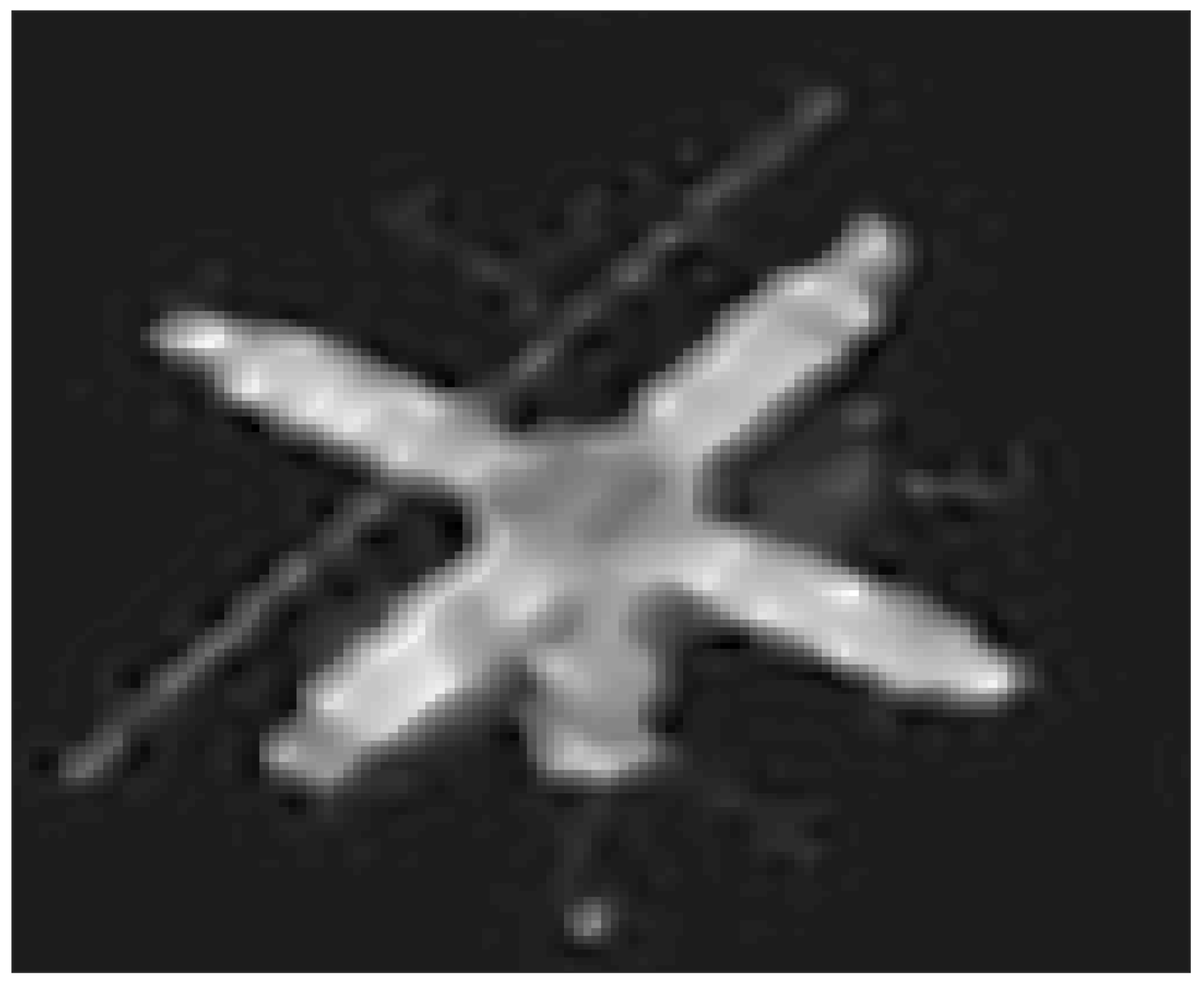
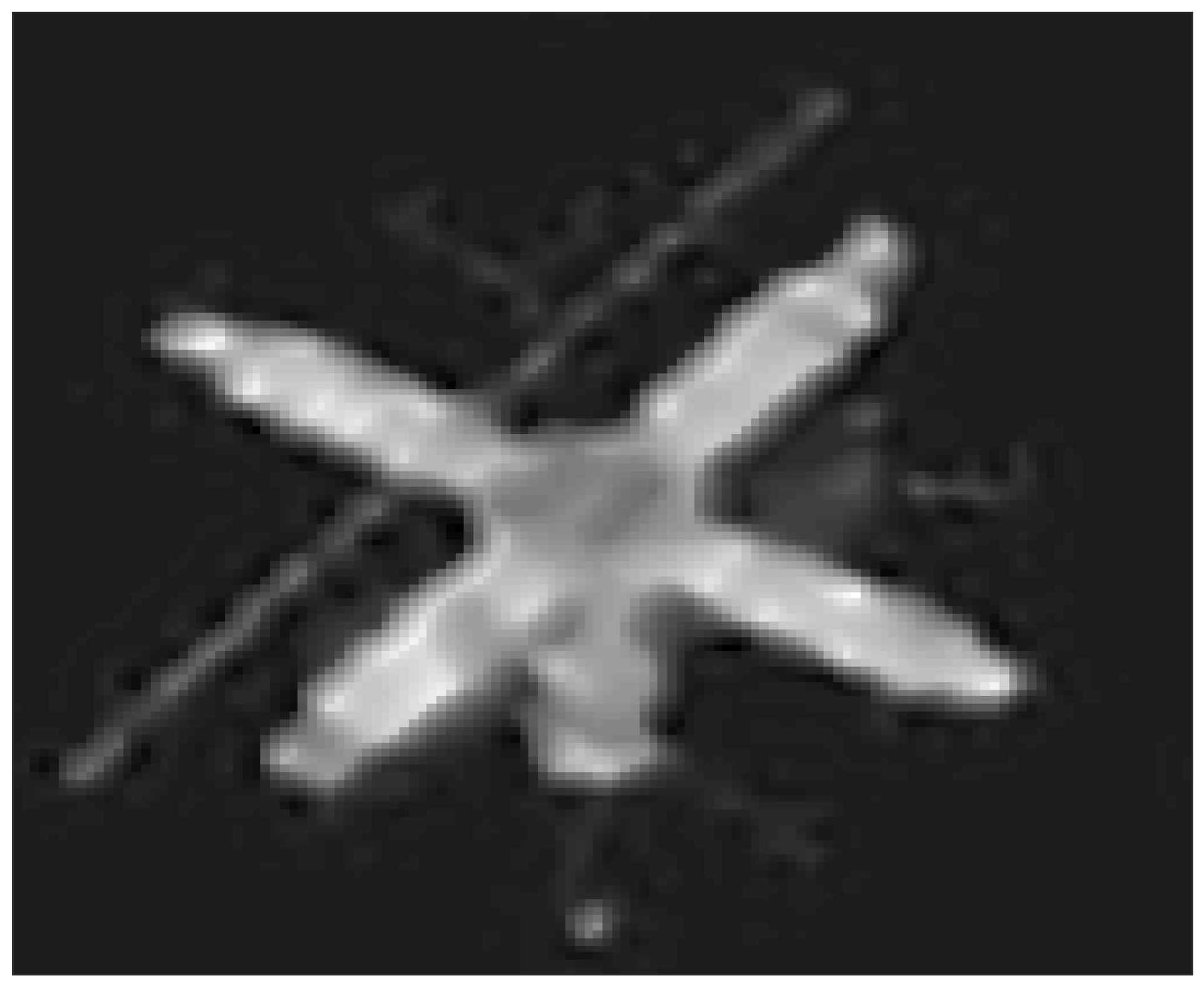
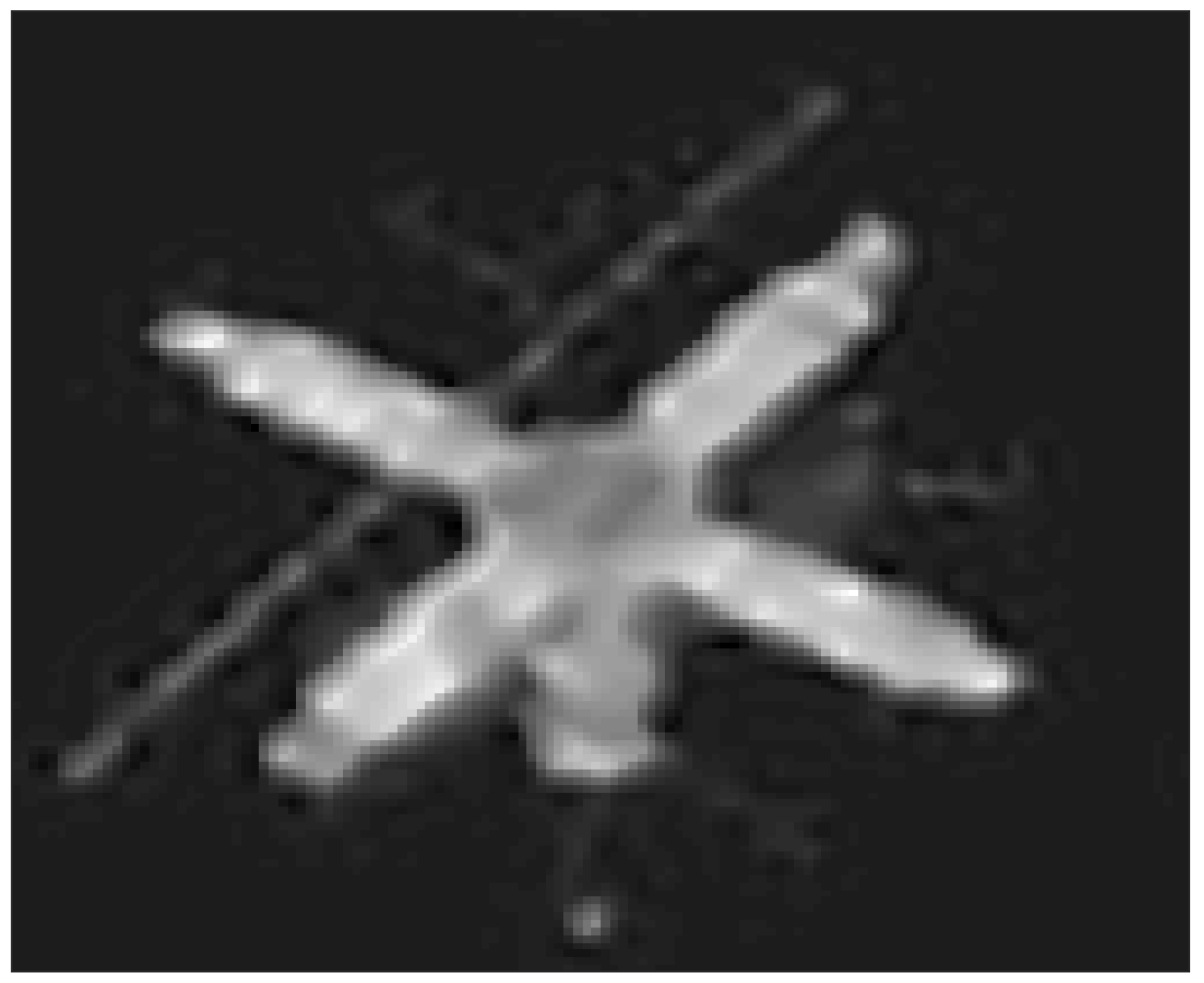
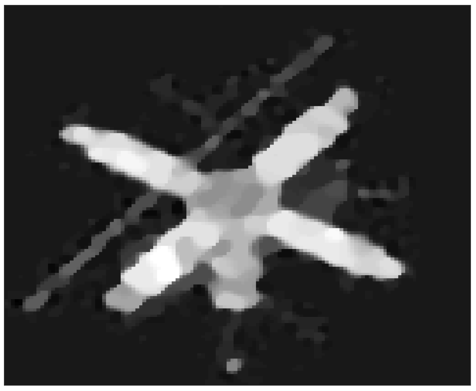
• We propose two block triangular preconditioners and study the bounds of the eigenvalues of the preconditioned matrices. In addition, we demonstrate the effectiveness of our algorithm in the numerical results by starting with the fixed point iteration (FPI) Method as in [28] to linearize the nonlinear primal system $\left[K^{T}K+\lambda L_h^{\alpha }\left(U^m\right)\right]U^{m+1}=K^{T}Z,m=0,1,\dots$, then we use the preconditioned conjugate gradient (PCG) method [29] for the inner iterations. After that, we use FGMRES method for the outer iterations. We illustrate the performance of our approach by calculating the peak signal-to-noise ratio (PSNR), CPU-time, residuals and the number of iterations. Finally, we calculate the PSNR for different values of the order of the fractional derivative, $\alpha$, to show the impact of using the TFOV model.

The remainder of this paper is organized as follows: Section 2 presents the mathematical model of the image deblurring problem, different regularization models, three definitions of the fractional derivative, and the Euler–Lagrange equations associated with the TFOV model. System (1) is obtained at the end of this section. Section 3 presents all theoretical contributions of this paper. Section 4 reports some numerical results that show the efficiency of our preconditioners. Section 5 briefly states our conclusions.

2. Problem Setup

We know that blurring and noise affect the quality of the received image. To deblur an image, we need a mathematical model of how it was blurred. The recorded image z and the true (exact) image $\mathbf{u}$ are related by the equation

$$z=\mathbf{K}\mathbf{u}+\epsilon ,$$

(2)

where $\mathbf{K}$ denotes the following blurring operator:

$$\left(\mathbf{K}\mathbf{u}\right)\left(x\right)={\int }_{\Omega }k(x,x^{\prime })\mathbf{u}\left(x^{\prime }\right)d{x}^{\prime },x\in \Omega$$

(3)

with translation-invariant kernel, $k(x,x^{\prime })=k(x-x^{\prime })$, known as the point spread function (PSF). $\epsilon$ is the additive noise function. $\Omega$ will denote a square in ${\mathcal{R}}^2$ on which the image intensity is defined. When $\mathbf{K}$ is the identity operator, the problem (2) becomes image de-noising. In this paper, we focus on de-blurring problem. The PSF function must be known. However, if it is unknown, another technique named blind deconvolution can be used [30]. The operator $\mathbf{K}$ is compact, so the problem (2) is ill-posed [31], and then the resulting matrix systems from the discretization of this problem are highly ill-conditioned. In this case, directly solving this problem is difficult. The most popular approach to obtain a well-posed problem is to add a regularization term. Different regularization terms are used in the literature, for example:

• Tikhonov regularization [32] is used to stabilize the problem (2) and also called as penalized least squares. In this case, the problem is then to find a u that minimize the functional

  $$F\left(u\right)=\frac{1}{2}{\Vert \mathbf{K}u-z\Vert }^2+\lambda J\left(u\right),$$

  (4)

  with a small positive parameter $\lambda$ called the regularization parameter that controls the trade-off between the data fitting term (the first term) and the regularization term (the second term). $\Vert ·\Vert$ denotes the norm in ${\mathcal{L}}^2(\Omega )$. The functional J has to be known. Common choices for the functional J are

  $$J\left(u\right)={\int }_{\Omega }{u}^{2}dx,$$

  (5)

  the above functional gives what is known as Tikhonov regularization with the identity, and

  $$J\left(u\right)={\int }_{\Omega }\mid \nabla u{\mid }^{2}dx,$$

  (6)

  where $\mid ·\mid$ denotes Euclidean norm, and $\nabla =\left(\frac{\partial }{\partial x},\frac{\partial }{\partial y}\right)$. When u is discontinuous, the functional in (5) often induces either oscillations or ringing. However, in the functional (6), we need to assume that u is a smooth function. Although, this model is easy to use and simple to calculate, it cannot preserve image edges. Hence, both the above choices are unsuitable for image processing applications when we need to recover sharp contrasts modeled by discontinuities in u [28].
• Total Variation (TV): One of the most commonly used regularization models is the TV. It was introduced for the first time [33] in edge-preserving image denoising by Rudin, Osher and Fatemi (ROF) and it has improved in recent years for image de-noising, de-blurring, in-painting, blind de-convolution, and processing [1,2,3,4,34,35,36,37,38,39]. When using the TV model, the problem is then to find a u that minimizes the functional

  $$F\left(u\right)=\frac{1}{2}{\Vert \mathbf{K}u-z\Vert }^2+\lambda J_{TV}\left(u\right),$$

  (7)

  where

  $$J_{TV}\left(u\right)={\int }_{\Omega }\mid \nabla u\mid dx.$$

  (8)
  Note that, we do not require the continuity of u. Hence, (8) is a good regularization in image processing. However, the Euclidean norm, $\mid \nabla u\mid$, is not differentiable at zero. Common modification is to add a small positive parameter $\beta$. The resulting is in the modified functional:

  $${J_{TV}}_{\beta }\left(u\right)={\int }_{\Omega }\sqrt{\mid \nabla u{\mid }^2+{\beta }^2}dx.$$

  (9)
  The well-posedness of the above minimization problem (7) with the functional given in (9) is studied and analyzed in the literature, such as in [1]. The success of using TV regularization is that TV gives a balance between the ability to describe piecewise smooth images and the complexity of the resulting algorithms. Moreover, the TV regularization performs very well for removing noise/blur while preserving edges. Despite the good contributions of the TV regularization mentioned above, it favors a piecewise constant solution in the bounded variation (BV) space which often leads to the staircase effect. Thus, stair casing remains one of the drawbacks of the TV regularization. To remove the stair case effects, two modifications to the TV regularization model have been used in the literature. The first approach is to higher the order of the derivatives in the TV regularization term, such as the mean curvature or a nonlinear combination of the first and second derivatives [40,41,42,43,44,45]. These modifications remove/reduce the staircase effects and they are effective but they are computationally expensive due to the increasing the order of the derivatives or due to the nonlinearity terms. The second approach is to use the fractional-order derivatives in the TV regularization terms as shown in [46,47].

2.1. Fractional-Order Derivative in Image Deblurring

The most important advantage of using fractional differential equations is their nonlocal property. The integer order differential operator is a local operator but the fractional order differential operator is nonlocal. This means that the next state of a system depends not only on its current state but also upon all of its historical states. This is more realistic and it is one reason why fractional calculus has become more and more popular.

In image deblurring problems, the blurring is considered nonlocal in some cases and local in others depending on the cause of the blur. For example, if a body is moving while the background is stationary, then the blur is local and in case the camera is moving then the blur is nonlocal. The blurring operator is a convolution operator that depends on the definition of the kernel functions. In the case of a moving camera, the blurring operator involves each pixel in the image, which means that the blurring process is a nonlocal. The bulrring is nonlocal, in this case, so it is appropriate to choose a regularization operator with the same nonlocal property. This property is available in operators that contain fractional derivatives. Comparative studies have shown that fractional-order differentials are more reliable than the integer-order differentials for enhancing edges in image processing. A similar trend has been observed for the texture and area-preserving properties. Therefore, images processed by fractional differentials are clearer and have higher contrast [48]. This approach is widely used in image processing [5,6,7,8,49,50]. These works have shown that the fractional-order derivative performs well in achieving a satisfactory compromise between avoiding staircasing and preserving important fine-scale features such as edges and textures. In this paper, we compare the results of the usual TV model with the TFOV model for two image deblurring problems. From Figure 1, Figure 2, Figure 3, Figure 4, Figure 5 and Figure 6, we can see that the TFOV shows better edge enhancement results than TV in some regions where we can observe that the PSNR at $\alpha =1$ is lower than PSNR at $\alpha >1$.

Example 1. 

We used the exact Golden House image plotted in Figure 9, the deblurred Golden House image using the TV-model plotted in Figure 27, and the deblurred Golden House image using the TFOV-model plotted in Figure 29. We took a vertical line almost in the middle of these images and plotted the results of the cross sections in Figure 1. In Figure 1, we highlighted three corners (boxes). From Figure 1, Figure 2, Figure 3, Figure 4, Figure 5 and Figure 6, we can clearly see that the TFOV-based image deblurring results are smoother than the TV-based image deblurring. Additionally, in each corner TV based image deblurring creates a higher error than TFOV. This shows that TFOV-based image deblurring is better and edge-preserving.

The numerical results in the above examples reflect good performance, and motivating us to use the TFOV model in our preconditioners.

2.2. The TFOV-Model

Let $B{V}^{\alpha }(\Omega )$ denotes the space of functions of $\alpha$-bounded variation on $\Omega$ defined by

$$B{V}^{\alpha }(\Omega ):=\left\{u\in L^1(\Omega )|T{V}^{\alpha }\left(u\right)<+\infty \right\}.$$

with the $B{V}^{\alpha }$ norm ${\left|\right|u\left|\right|}_{B{V}^{\alpha }}={\left|\right|u\left|\right|}_{L^1}+{\int }_{\Omega }\left|{\nabla }^{\alpha }u\right|dx$. The parameter $\alpha$ represents the order of the fractional derivatives, the fractional-order total variation of u, $T{V}^{\alpha }$ is defined by

$$T{V}^{\alpha }\left(u\right)={\int }_{\Omega }\left|{\nabla }^{\alpha }u\right|dx:=\underset{\varphi \in T}{sup}{\int }_{\Omega }\left(-udi{v}^{\alpha }\varphi \right)dx,$$

and $di{v}^{\alpha }\varphi =\frac{{\partial }^{\alpha }{\varphi }_1}{\partial x}+\frac{{\partial }^{\alpha }{\varphi }_2}{\partial y}$, $\frac{{\partial }^{\alpha }{\varphi }_1}{\partial x}$ and $\frac{{\partial }^{\alpha }{\varphi }_2}{\partial y}$ denote the fractional-order derivative along the x and y directions respectively. The space T denotes the space of special test functions

$$T:=\left\{\varphi \in C_0^{\ell }(\Omega ,{\mathbb{R}}^2)\left|\varphi \left(x\right)\right|\le 1,\forall x\in \Omega \right)$$

where $\left|\varphi \left(x\right)\right|=\sqrt{{\Sigma }_{i=1}^2{\varphi }_i^2}$ and $C^{\ell }(\Omega ,{\mathbb{R}}^2)$ denote the space of $\alpha$-order continuously differentiable functions. Hence, when the TFOV- model is used, the problem is then to find a $u\in {BV}^{\alpha }(\Omega )\cap L^2(\Omega )$ that minimizes the functional

$$\begin{array}{cc}\hfill F^{\alpha }\left(u\right)& =\frac{1}{2}{\Vert \mathbf{K}u-z\Vert }^2+\lambda {J_{TV}^{\alpha }}_{\beta }\left(u\right)\hfill \end{array}$$

(10)

where ${J_{TV}^{\alpha }}_{\beta }$ is called the modified total fractional-order variation and defined by

$${J_{TV}^{\alpha }}_{\beta }\left(u\right)={\int }_{\Omega }\sqrt{\mid {\nabla }^{\alpha }u{\mid }^2+{\beta }^2}dx,$$

(11)

where $|{\nabla }^{\alpha }{u|}^2={\left(D_x^{\alpha }u\right)}^2+{\left(D_y^{\alpha }u\right)}^2$ where $D_x^{\alpha },D_y^{\alpha }$ are the fractional derivative operators along the x and y directions respectively. Existence and uniqueness of a minimizer to the above problem (10) with the functional (11) are studied and analyzed in the literature [8,51].

2.3. Fractional-Order Derivatives

Several definitions have been proposed for fractional-order derivatives [52,53,54]. We shall present some of them below. For a systematic presentation of mathematics, a fractional-order derivative is denoted as function operator ${D^{\alpha }}_{[a,x]}$, where a and x are the bounds of the integrals, and $\alpha$ is the order of the fractional derivative such that $0<n-1<\alpha <n$ where $n=\left[\alpha \right]+1$ and $[·]$ is the greatest integer function.

• Riemann–Liouville (RL) definitions: The left- and right-sided RL derivatives of order $\alpha$ of a function $f\left(x\right)$ are given as follows:

  $${D^{\alpha }}_{[a,x]}f\left(x\right)=\frac{1}{\Gamma (n-\alpha )}{\left(\frac{d}{dx}\right)}^n{\int }_a^x{(x-t)}^{n-\alpha -1}f\left(t\right)dt$$

  (12)

  and

  $${D^{\alpha }}_{[x,b]}f\left(x\right)=\frac{{(-1)}^n}{\Gamma (n-\alpha )}{\left(\frac{d}{dx}\right)}^n{\int }_x^b{(t-x)}^{n-\alpha -1}f\left(t\right)dt$$

  (13)

  where $\Gamma (·)$ is the gamma function, defined by

  $$\Gamma \left(z\right)={\int }_0^{\infty }{e}^{-t}{t}^{z-1}dt.$$
• Grünwald–Letnikov (GL) definitions: The left- and right-sided GL derivatives are defined by

  $${}^G{D}_{[a,x]}^{\alpha }f\left(x\right)=\underset{h\to 0}{lim}\frac{{\Sigma }_{j=0}^{\left[\frac{x-a}{h}\right]}{(-1)}^j{C}_{\alpha }^{j}f(x-jh)}{h^{\alpha }}$$

  (14)

  and

  $${}^G{D}_{[x,b]}^{\alpha }f\left(x\right)=\underset{h\to 0}{lim}\frac{{\Sigma }_{j=0}^{\left[\frac{b-x}{h}\right]}{(-1)}^j{C}_{\alpha }^{j}f(x+jh)}{h^{\alpha }}$$

  (15)

  where

  $$C_{\alpha }^j=\frac{\alpha (\alpha -1)\dots (\alpha -j+1)}{j!}.$$

  (16)
• Caputo (C) definitions: The left- and right-sided Caputo derivatives are defined by

  $${}^C{D}_{[a,x]}^{\alpha }f\left(x\right)=\frac{1}{\Gamma (n-\alpha )}{\int }_a^x{(x-t)}^{n-\alpha -1}{f}^{\left(n\right)}\left(t\right)dt$$

  (17)

  and

  $${}^C{D}_{[x,b]}^{\alpha }f\left(x\right)=\frac{{(-1)}^n}{\Gamma (n-\alpha )}{\int }_x^b{(t-x)}^{n-\alpha -1}{f}^{\left(n\right)}\left(t\right)dt$$

  (18)

  where $f^{\left(n\right)}$ denotes the $n\mathrm{th}$-order derivative of function $f\left(x\right)$.

2.4. Euler-Lagrange Equations

In this subsection, we present the Euler-Lagrange equations associated with the TFOV in image de-blurring problem.

Theorem 1. 

If $\alpha \in (1,2)$, the Euler-Lagrange equations for the functional given in (10) are:

$$\begin{array}{cc}\hfill & {\mathit{K}}^{*}(\mathit{K}u-z)+\lambda L_{\alpha }\left(u\right)u=0,in\Omega \hfill \\ \hfill & D^{\alpha -2}\left(\frac{{\nabla }^{\alpha }u}{\sqrt{|{\nabla }^{\alpha }{u|}^2+{\beta }^2}}\right)·\overrightarrow{n}=0,D^{\alpha -1}\left(\frac{{\nabla }^{\alpha }u}{\sqrt{|{\nabla }^{\alpha }{u|}^2+{\beta }^2}}\right)·\overrightarrow{n}=0,on\partial \Omega ,\hfill \end{array}$$

(19)

where ${\mathit{K}}^{*}$ is the adjoint operator of the integral operator $\mathit{K}$ and the nonlinear deferential operator $L_{\alpha }\left(u\right)$ is given by:

$$L_{\alpha }\left(u\right)w={(-1)}^n{\nabla }^{\alpha }.\left(\frac{{\nabla }^{\alpha }w}{\sqrt{|{\nabla }^{\alpha }{u|}^2+{\beta }^2}}\right).$$

(20)

Proof. 

Let $\nu \in W_1^{\alpha }(\Omega )$ be a function. Then for $u\in W_1^{\alpha }(\Omega )\subset B{V}^{\alpha }(\Omega )$, the first order Gateaux derivative of the functional $F^{\alpha }\left(u\right)$ of (10) in the direction of $\nu$ is

$$\frac{\partial F^{\alpha }\left(u\right)\nu }{\partial \nu }=li{m}_{t\to 0}\frac{F^{\alpha }(u+t\nu )-F^{\alpha }\left(u\right)}{t}$$

(21)

$$=\underset{t\to 0}{lim}\frac{G_1(u+t\nu )-G_1\left(u\right)}{t}+\underset{t\to 0}{lim}\frac{G_2(u+t\nu )-G_2\left(u\right)}{t},$$

where $G_1\left(u\right)=\frac{1}{2}{\int }_{\Omega }^{}(\mathbf{K}u-z)dx$ and $G_2\left(u\right)=\lambda J_{TV\beta }^{\alpha }\left(u\right)$. By using the Taylor series in the direction of t, we have

$$\frac{\partial F^{\alpha }\left(u\right)\nu }{\partial \nu }={\int }_{\Omega }^{}{\mathbf{K}}^{*}(\mathbf{K}u-z)dx+{\int }_{\Omega }^{}(\mathbf{W}.{▽}^{\alpha }\nu )dx,$$

(22)

where $\mathbf{W}=\lambda \frac{{\nabla }^{\alpha }u}{\sqrt{|{\nabla }^{\alpha }{u|}^2+{\beta }^2}}$. Now consider,

$${\int }_{\Omega }^{}(\mathbf{W}.{▽}^{\alpha }\nu )dx={(-1)}^n{\int }_{\Omega }^{}\left({\nu }^{C}di{v}^{\alpha }\mathbf{W}\right)dx$$

(23)

$$-\sum _{j=0}^{n-1}{(-1)}^j{\int }_0^1{D}_{[a,b]}^{\alpha +j-n}{W}_1\frac{{\partial }^{n-j-1}\nu \left(x\right)}{\partial x_1^{n-j-1}}{|}_{x_1=0}^{x_1=1}d{x}_2-\sum _{j=0}^{n-1}{(-1)}^j{\int }_0^1{D}_{[a,b]}^{\alpha +j-n}{W}_2\frac{{\partial }^{n-j-1}\nu \left(x\right)}{\partial x_2^{n-j-1}}{|}_{x_2=0}^{x_2=1}d{x}_1,$$

where we know that $n=2$ for $1<\alpha <2$.

Case-I: If $u\left(x\right){|}_{\partial \Omega }=b_1\left(x\right)$ and $\frac{\partial u\left(x\right)}{\partial n}{|}_{\partial \Omega }=b_2\left(x\right)$, so $\left(u\left(x\right)+t\nu \left(x\right)\right){|}_{\partial \Omega }=b_1\left(x\right)$ and $\frac{\partial \left(u\left(x\right)+t\nu \left(x\right)\right)}{\partial n}{|}_{\partial \Omega }=b_2\left(x\right)$. Then it suffices to take $\nu \in {\mathcal{C}}_0^1(\Omega ,\mathbb{R})$, this implies

$$\frac{{\partial }^i\nu \left(x\right)}{\partial n^i}{|}_{\partial \Omega }=0,i=0,1,$$

$$\Rightarrow \frac{{\partial }^{n-j-1}\nu \left(x\right)}{\partial x_1^{n-j-1}}{|}_{x_1=0,1}=\frac{{\partial }^{n-j-1}\nu \left(x\right)}{\partial x_2^{n-j-1}}{|}_{x_2=0,1}=0,n-j-1=0,1.$$

Hence (22) reduces to (19).

Case-II: If $\nu \in W_1^{\alpha }(\Omega )$, then

$$\frac{{\partial }^{n-j-1}\nu \left(x\right)}{\partial x_1^{n-j-1}}{|}_{x_1=0,1}\ne 0,\frac{{\partial }^{n-j-1}\nu \left(x\right)}{\partial x_2^{n-j-1}}{|}_{x_2=0,1}\ne 0,n-j-1=0,1.$$

So boundary terms in (23) can only become zero if

$$D_{[a,b]}^{\alpha +j-n}{W}_1{|}_{x_1=0,1}=D_{[a,b]}^{\alpha +j-n}{W}_2{|}_{x_2=0,1}=0$$

$$\Rightarrow D^{\alpha +j-n}\mathbf{W}.n=0,j=0,1.$$

This completes the proof. □

Note that (19) is a nonlinear integro-differential equation of elliptic type. Equation (19) can be expressed as a nonlinear first order system [55]:

$${\mathbf{K}}^{*}\mathbf{K}u+\lambda {\nabla }^{\alpha }.\overrightarrow{v}={\mathbf{K}}^{*}z,$$

(24)

$$-{\nabla }^{\alpha }u+\sqrt{\mid {\nabla }^{\alpha }u{\mid }^2+\beta }\overrightarrow{v}=\overrightarrow{0},$$

(25)

with the dual, or flux, variable

$$\overrightarrow{v}=\frac{{\nabla }^{\alpha }u}{\sqrt{\mid {\nabla }^{\alpha }u{\mid }^2+\beta }}.$$

(26)

We apply the Galerkin method to (24) and (25) together with the midpoint quadrature for the integral term and cell-centered finite difference method for the derivative part.

2.5. Discretization of the Fractional Derivative

First, we divide the square domain $\Omega =(0,1)\times (0,1)$ into $N^2$ equal squares (cells) where N denotes the number of equispaced partitions in the x or y directions. Then, we follow the same discretization in [8,51]. We define a spatial partition $(x_k,y_l)$ (for all $k,l=0,1,\dots ,N+1$) of image domain $\Omega$. Assume u has a zero Dirichlet boundary condition, we consider the discretization of the $\alpha$-order fractional derivative at the inner point $(x_k,y_l)$ (for all $k,l=0,1,\dots ,N$) on $\Omega$ along the x-direction by using the shifted Gr$ü$nwald approximation approach [56,57]

$$\begin{array}{cc}\hfill D^{\alpha }f(x_k,y_l)& =\frac{{\delta }_0^{\alpha }f(x_k,y_l)}{h^{\alpha }}+O\left(h\right)=\frac{1}{2}\left(\frac{{\delta }_{-}^{\alpha }f(x_k,y_l)}{h^{\alpha }}+\frac{{\delta }_{+}^{\alpha }f(x_k,y_l)}{h^{\alpha }}\right)+O\left(h\right)\hfill \\ \hfill & =\frac{1}{2h^{\alpha }}\left({\Sigma }_{j=0}^{k+1}{\omega }_j^{\alpha }{f}_{k-j+1}^l+{\Sigma }_{j=0}^{N-k+2}{\omega }_j^{\alpha }{f}_{k+j-1}^l\right)+O\left(h\right)\hfill \end{array}$$

(27)

where $f_s^l=f_{s,l}$ and ${\omega }_j^{\alpha }={(-1)}^j\left(\begin{array}{c}\alpha \\ j\end{array}\right)j=0,1,\dots ,N$ and ${\omega }_0^{\alpha }=1,{\omega }_j^{\alpha }=(1-\frac{1+\alpha }{j}){\omega }_{j-1}^{\alpha }$ for $j>0$. Observe from (27) that the first order estimate of the $\alpha$-order fractional derivative ${D_{[a,b]}}^{\alpha }f(x_k,y_l)$ along the x-direction at the point $(x_k,y_l)$ with a fixed $y_l$ is a linear combination of $N+2$ values ${f^l}_0,{f^l}_1,\dots ,{f^l}_N,{f^l}_{N+1}$. After incorporating the zero boundary condition in the matrix approximation of fractional derivative, all N equations of fractional derivatives along the x direction in (27) can be written simultaneously in the matrix form

$$\begin{array}{cc}\hfill & \left[\begin{array}{c}{\delta }_0^{\alpha }f(x_1,y_l)\\ {\delta }_0^{\alpha }f(x_2,y_l)\\ ⋮\\ ⋮\\ {\delta }_0^{\alpha }f(x_N,y_l)\end{array}\right]=\hfill \\ & \underset{{B^{\alpha }}_N}{\underbrace{\frac{1}{2h^{\alpha }}\left[\begin{array}{ccccc}2{{\omega }_1}^{\alpha }& {{\omega }_0}^{\alpha }+{{\omega }_2}^{\alpha }& {{\omega }_3}^{\alpha }& \cdots & {{\omega }_N}^{\alpha }\\ {{\omega }_0}^{\alpha }+{{\omega }_2}^{\alpha }& 2{{\omega }_1}^{\alpha }& \ddots & \ddots & ⋮\\ {{\omega }_3}^{\alpha }& \ddots & \ddots & \ddots & {{\omega }_3}^{\alpha }\\ ⋮& \ddots & \ddots & 2{{\omega }_1}^{\alpha }& {{\omega }_0}^{\alpha }+{{\omega }_2}^{\alpha }\\ {{\omega }_N}^{\alpha }& \cdots & {{\omega }_3}^{\alpha }& {{\omega }_0}^{\alpha }+{{\omega }_2}^{\alpha }& 2{{\omega }_1}^{\alpha }\end{array}\right]}}\left[\begin{array}{c}{f}_1^l\\ f_2^l\\ ⋮\\ ⋮\\ f_N^l\end{array}\right].\hfill \end{array}$$

From the definition of fractional-order derivative (27), for any $1<\alpha <2$, the coefficients ${{\omega }_k}^{\alpha }$ have the following properties:

(1)

${{\omega }_0}^{\alpha }=1,{{\omega }_1}^{\alpha }=-\alpha <0,1\ge {{\omega }_2}^{\alpha }\ge {{\omega }_3}^{\alpha }\ge \dots \ge 0.$

(2)

${\sum }_{k=0}^{\infty }{{\omega }_k}^{\alpha }=0,{\sum }_{k=0}^m{{\omega }_k}^{\alpha }\le 0(m\ge 1)$.

Hence by the Gershgorin circle theorem, we can derive that matrix ${B^{\alpha }}_N$ is a symmetric and negative definite Toeplitz matrix (i.e., $-{B^{\alpha }}_N$ is a positive definite Toeplitz matrix). Let $U\in {\mathbb{R}}^{N\times N}$ denote the solution matrix at all nodes $(khx;lhy),k,l=1,\dots ,N$ corresponding to x-direction and y-direction spatial discretization nodes. Denote by $\overrightarrow{u}\in {\mathbb{R}}^{N^2\times 1}$, the ordered solution vector of U. The direct and discrete analogue of differentiation of arbitrary $\alpha$ order derivative is

$${u_x}^{\alpha }=(I_N\otimes {B^{\alpha }}_N)\overrightarrow{u}={B_x}^{\alpha }\overrightarrow{u}$$

(28)

Similarly, all values of $\alpha$-th order y-direction derivative of $u(x;y)$ at these nodes are approximated by

$${u_y}^{\alpha }=({B^{\alpha }}_N\otimes I_N)\overrightarrow{u}={B_y}^{\alpha }\overrightarrow{u},$$

(29)

where

$${u_x}^{\alpha }={({u_{11}}^{\alpha },\dots ,{u_{N1}}^{\alpha },{u_{12}}^{\alpha },\dots ,{u_{NN}}^{\alpha })}^T,{u_y}^{\alpha }={({u_{11}}^{\alpha },\dots ,{u_{1N}}^{\alpha },{u_{21}}^{\alpha },\dots ,{u_{NN}}^{\alpha })}^T,$$

(30)

$\overrightarrow{u}=u_{11},u_{12},\dots ,u_{NN}$ and ⊗ denotes the Kronecker product. For more details in the discretization, we refer to [54,58]. Now, using the cell center finite difference Method (CCFDM), the fractional discretization shown above, and using the fact that $[{(-1)}^n{\nabla }^{\alpha }·]$ is the adjoint operator of the operator ${\nabla }^{\alpha }$, then (24) and (25) leads to the following system

$$\begin{array}{cc}\hfill & V+K_{h}U=Z,\hfill \\ \hfill & K_h^{*}V-\lambda \left({L^{\alpha }}_h{U}^m\right)U^{m+1}=0,m=0,1,2\dots N_F,\hfill \end{array}$$

(31)

where $N_F$ is the number of Fixed-Point Iterations used to linearize the nonlinear term in the square root in (26). The matrix $K_h$ is obtained form using the midpoint quadrature for the integral operator as follows:

$$\left(\mathbf{K}u\right)(x_i,y_j)\approx {\left[K_{h}U\right]}_{ij},i,j=1,2,\dots ,N.$$

(32)

with entries ${\left[K_{h}U\right]}_{ij,lm}=h^{2}k(x_i-x_j,y_l-y_m)$. With using the lexicographical order, $K_h$ is a block Toeplitz with Toeplitz block (BTTB) matrix. The need for BTTB property will be discussed later in the paper. The discrete scheme of the matrix ${L^{\alpha }}_{h}U$ is given by:

$$\begin{array}{c}\hfill \left(L^{\alpha }\left(U^m\right)\right)U^{m+1}=[B_N\left(D_1\left(U^m\right)\right)\circ \left(B_N{U}^{m+1}\right)]+\left[(D_2\left(U^m\right)\circ \left(U^{m+1}{B}_M\right))\right]B_N\end{array}$$

(33)

where ∘ is the point wise multiplication and m is the $m\text{-}\mathrm{th}$ Fixed-Point Iteration. U is an $N\times N$-size reshaped matrix of the vector u and the matrices $D_1\left(U^m\right)$ and $D_2\left(U^m\right)$ are the diagonal of the Hadamard inverses of the non-zero matrices ${B_x}^{\alpha }\left(U^m\right)$ and ${B_y}^{\alpha }\left(U^m\right)$ respectively.

2.6. Difficulties in TFOV-Model Compared to TV-Model

In this subsection, we compare the TFOV-system (1):

$$\underset{{\mathrm{A}}^{\alpha }}{\underbrace{\left[\begin{array}{cc}{I}_n\hfill & K_h\hfill \\ -K_h^{*}\hfill & \lambda L_h^{\alpha }\left(U_h\right)\hfill \end{array}\right]}}\underset{\mathrm{x}}{\underbrace{\left[\begin{array}{c}{V}_h\hfill \\ U_h\hfill \end{array}\right]}}=\underset{\mathrm{b}}{\underbrace{\left[\begin{array}{c}{Z}_h\hfill \\ 0\hfill \end{array}\right]}},$$

and the following TV-system:

$$\underset{\mathrm{A}}{\underbrace{\left[\begin{array}{cc}{I}_n\hfill & K_h\hfill \\ -K_h^{*}\hfill & \lambda L_h\left(U_h\right)\hfill \end{array}\right]}}\underset{\mathrm{x}}{\underbrace{\left[\begin{array}{c}{V}_h\hfill \\ U_h\hfill \end{array}\right]}}=\underset{\mathrm{b}}{\underbrace{\left[\begin{array}{c}{Z}_h\hfill \\ 0\hfill \end{array}\right]}}.$$

(34)

In the TFOV system (1), the fractional matrix $L_h^{\alpha }$ is obtained from discretizing a fractional deferential operator and it is dense. The density property leads to an expensive matrix-vector multiplication. In this case, the coefficient matrix $A^{\alpha }$ in the system (1) contains three dense submatrices, while in TV system (34), the non-fractional matrix $L_h$ is obtained from discretizing a non-fractional deferential operator and it is a sparse matrix, then the coefficient matrix A in the system (34) contains only two dense submatrices. Further, the Schur complement matrix associated with (1) is a sum of two dense matrices while the Schur complement matrix associated with (34) is a sum of one dense matrix and one sparse matrix.

3. Preconditioning Technique

In the literature, it has been shown that block triangular preconditioners are among the most effective preconditioners for solving saddle point problems. In this paper, we develop two block triangular preconditioners for solving (1). First, we present our main preconditioner matrix [12] and its inverse:

$$P=\left[\begin{array}{cc}{I}_n& K\\ 0& -S\end{array}\right],P^{-1}=\left[\begin{array}{cc}{I}_n& K{S}^{-1}\\ 0& -S^{-1}\end{array}\right],$$

(35)

where $S=K^{*}K+\lambda L_{\alpha }$ is the Schur complement matrix. We notice that the Schur complement matrix contains the product $\left(K{}^{*}K\right)$ which is not a BTTB matrix. We know that a BTTB matrix-vector product computation cost $O(NlogN)$ but using a BCCB extension. Since this extension is not an easy task in some cases, the idea of using a circulant matrix as a preconditioner for a Toeplitz matrix is needed. This idea was first proposed by Strang [59] and Olkin [60] and extended by others to block Toeplitz systems for example Chan et al. [61]. Many researchers use Toeplitz preconditioners and block Toeplitz preconditioners for Toeplitz systems. For instance, Chan et al. [62], and Lin and Fu-Rong [63]. Band Toeplitz preconditioner and band BTTB preconditioner are proposed by Chan and Raymond [64] and Serra and Stefano [65]. In Lin et al. [66], BTTB preconditioners for BTTB systems are discussed. Several kinds of circulant preconditioners have been proposed to be good preconditioners, see for instance [59,62,67,68,69]. Several kinds of circulant preconditioners have been proposed and proven to be good preconditioners. Therefore, the PCG methods with circulant preconditioners converge very fast when they are used to solve Toeplitz systems. Motivated by these papers, we propose the following two block triangular preconditioners:

$$P_1=\left[\begin{array}{cc}{I}_n& K\\ 0& -S_1\end{array}\right],P_2=\left[\begin{array}{cc}{I}_n& K\\ 0& -S_2\end{array}\right],$$

(36)

where $S_1=(I+\lambda L_{TV})$ and $S_2=(C^{*}C+\lambda L_{TV})$. Where I is the denoising operator, the identity matrix is a circulant matrix, and $L_{TV}$ comes from discretaizing the TV model $(\alpha =1)$ which is a sparse matrix and C is the Strang circulant approximation of the matrix K [59]. These circulant approximations are very important to allow us to use the FFT and the convolution theorem. We know that all circulant matrices can be diagonalized by the Fourier matrix, see [70]. Also using FFT and the convolution theorem will reduce the cost of the computation from $O\left(N^2\right)$ into $O(NlogN)$. Moreover, all that is needed for computation is the first column or the first row of the circulant matrix, which decreases the amount of required storage. This reduction in the computations and storage leads to efficient solvers for our problem (1).

4. Preconditioned GMRES Algorithm

In this section, we give a detailed algorithms for using our preconditioner P ($P_1$ and $P_2$). In Algorithm 1, GMRES method is used to solve the linear system (1).

Algorithm 1 Preconditioned GMRES Algorithm

1: Choose $x^0$ as the initial guess 2: Compute ${\tilde{r}}^0=b-A{x}^0$ 3: Solve P$r^0={\tilde{r}}^0$ 4: Let ${\beta }_0=\parallel r^0\parallel ,$ and compute $v^{\left(1\right)}=r^0/{\beta }_0$ 5: for $k=1,2,\dots$ until ${\beta }_k<\tau {\beta }_0$ do 6:      ${\tilde{w}}_0^{(k+1)}=A{v}^{\left(k\right)}$ 7:      Solve P $w_0^{(k+1)}={\tilde{w}}_0^{(k+1)}$ 8:      for $l=1$ to k do 9:            $h_{lk}=\langle {w_l}^{(k+1)},v^{\left(l\right)}\rangle$ 10:          ${w_l}^{(k+1)}={w_l}^{(k+1)}-h_{lk}{v}^{\left(l\right)}$ 11:      end for 12:      $h_{k+1,k}=w_{k+l}^{(k+1)}/h_{k+1,k}$ 13:      Compute $y^{\left(k\right)}$ such that ${\beta }_k=\parallel {\beta }_0{e}_1-{\widehat{H}}_k{y}^{\left(k\right)}\parallel$ is minimized, where   ${\widehat{H}}_k={\left[h_{ij}\right]}_{1\le i\le k+1\le ,1\le j\le k}$ and $e_1={(1,0,\dots ,0)}^T$ 14: end for 15: $x^{\left(k\right)}=x^0+V_k{y}^{\left(k\right)}$

In Algorithm 1, in Steps 3 and 7, we need to solve a matrix times a vector of the form

$$\underset{P}{\underbrace{\left[\begin{array}{cc}{I}_n\hfill & K\hfill \\ 0\hfill & -S\hfill \end{array}\right]}}\underset{\mathrm{x}}{\underbrace{\left[\begin{array}{c}{x}_1\hfill \\ x_2\hfill \end{array}\right]}}=\underset{\mathrm{b}}{\underbrace{\left[\begin{array}{c}{b}_1\hfill \\ b_2\hfill \end{array}\right]}},$$

(37)

where $S=S_1$ or $S=S_2$. To do the above multiplications, we use the conjugate gradients method as in Algorithms 2 and 3:

Algorithm 2 $P_1$-Conjugate Gradient Method Algorithm

1: $x_1=x(1:n)=b(1:n)-K{x}_2;$ 2: $S_1=P_1(n+1:2n,n+1:2n);$ 3: $b_2=b(n+1:2n);$ 4: $x_2=x(n+1:2n)$ 5: Solve for $x_2$ in the system $-S_{1}x{}_2=b_2$ using conjugate gradient method.

Algorithm 3 $P_2$-Conjugate Gradient Method Algorithm

1: $x_1=x(1:n)=b(1:n)-K{x}_2;$ 2: $S_2=P_2(n+1:2n,n+1:2n);$ 3: $b_2=b(n+1:2n);$ 4: $x_2=x(n+1:2n)$; 5: Solve for $x_2$ in the system $-S_{2}x{}_2=b_2$ using conjugate gradient method.

Eigenvalues Estimates

In this subsection, we need to study the eigenvalues of the exact preconditioned matrix $P^{-1}A$. Since $P^{-1}A$ and $A{P}^{-1}$ are similar matrices, they have the same eigenvalues. Hence we study the eigenvalues of the matrix $A{P}^{-1}$.

Theorem 2. 

If the linear system (1) is left preconditioned by the matrix P, then the preconditioned matrix is

$$A{P}^{-1}=\left[\begin{array}{cc}{I}_n& 0\\ -K^{*}& -I_n\end{array}\right],$$

(38)

and its minimal polynomial is $(\nu -1)(\nu +1)$ where ν is the eigenvalue of the matrix $A{P}^{-1}$.

Proof. 

Since $A{P}^{-1}$ and $P^{-1}A$ are similar, it is easy to study the eigenvalues of $A{P}^{-1}$ instead of $P^{-1}A$. From the form of $A{P}^{-1}$, we notice that the preconditioned matrix has only two distinct eigenvalues $\pm 1$ and then we notice that a minimal polynomial of degree at most 2. Hence, when Krylov subspace methods like FGMRES is used, then it converges in 2 iterations or less, in exact arithmetic. This property is of practical use when inexpensive approximations of the Schur complement exist. However, when we approximate the Schur complement matrix S by the matrix $S_1$ or $S_2$, we have the following eigenvalue estimation. □

Theorem 3. 

If the linear system (1) is left preconditioned by the matrix $P_1$ or $P_2$, then the eigenvalues of the preconditioned matrices

$$A{\left(P_1\right)}^{-1}=\left[\begin{array}{cc}{I}_n& 0\\ -K^{*}& -S{S_1}^{-1}\end{array}\right],andA{\left(P_2\right)}^{-1}=\left[\begin{array}{cc}{I}_n& 0\\ -K^{*}& -S{S_2}^{-1}\end{array}\right]$$

(39)

are described as follows:

$${\nu }_{+}=\left\{1\right\},and{\nu }_{-}\in [{\sigma }_1,{\sigma }_n],$$

(40)

where ${\sigma }_1$ and ${\sigma }_n$ are the minimum and the maximum eigenvalues of the matrix $(-S{S_1}^{-1})$ or $(-S{S_2}^{-1})$.

Example 2. 

In this example, our aim is to verify that the bounds given in the above theorem are matched. We take $N=16,i.e.,n={\left(16\right)}^2=256$ and we fix $\alpha =1.4,\beta =0.1,\lambda =0.001$. For this task, we use the preconditioner $P_1$ and we use the test image “Golden House”. We notice that the positive eigenvalues are equal to one whereas the negatives are contained in the interval $[{\sigma }_1,{\sigma }_n]$ where ${\sigma }_1$ and ${\sigma }_n$ are defined in the above theorem. In this example ${\sigma }_1\cong -1.01$ and ${\sigma }_n\cong -1$. The results of this example are plotted and shown in Figure 7 and Figure 8. Moreover, in this experiment, we find that the $cond\left(A\right)=3.2915\times {10}^4$ and $cond\left({\left(P_1\right)}^{-1}A\right)=1.6219$ which indicate that our preconditioner is effective.

From Figure 7 and Figure 8, we notice that the preconditioned matrix has a good clustering behavior of the eigenvalues. The eigenvalues are clustering around 1 and $-1$. This clustering verifies the above theorem guarantees fast convergence of the FGMRES method.

5. Numerical Results

In this section, we experimentally study the performance of the FGMRES method with the proposed preconditioners $P_1$ and $P_2$. In the following numerical experiments, we implement Algorithms 1–3, and we take the zero vector to be the initial guess. We stopped the outer iterations (FGMRES) when the residuals satisfies $\parallel b-A{x}^k\parallel <{10}^{-7}\Vert b\Vert$ where $x^k=(v^k,u^k)$ is the solution vector in the $k\text{-}\mathrm{th}$ iteration. We used only one iteration of the Fixed-Point Iteration method to linearize the nonlinear term and then we used the PCG for the inner iterations and it is stopped when the tolerance is ${10}^{-9}$. No restarting is used for FGMRES algorithm. For this purpose, two famous $128\times 128$ test images, called Retinal Image and Golden House are used in the experiments, as shown in Figure 9 and Figure 10 and they are blurred by the motion kernel as shown in Figure 11.

In order to show the performance of the proposed preconditioners, we need to calculate the PSNR which is commonly used in the signal processing field. It can be calculated by the following formula:

$$PSNR(u_e,u_d)=10log\left(\frac{n{max}_{1\le i,j\le n}\mid u_e\mid }{{\sum }_{i=1}^{n_x}{\sum }_{j=1}^{n_x}{\left({u_e}_{ij}-{u_d}_{ij}\right)}^2}\right)$$

(41)

where $u_e$ and $u_d$ are the exact and deblurred images, respectively. Bigger PSNR means better deblurring performance.

5.1. The Parameters $\beta$ and $\lambda$ Selecting

The value of the parameters $\beta$ and $\lambda$ also play a vital role in the performance of the numerical technique used for the image deblurring model. Small values of $\beta$ affect the convergence rate of the iterations in the numerical technique but do not change the quality of the deblurred images. We have chosen $\beta =1,\beta =0.1$ and $\beta =0.01$ which are commonly used in the literature [28]. We noticed no significant difference in the results between these values. Regarding the values of the regularization parameters $\lambda$, we have chosen $\lambda$ small enough, ${10}^{-3}$, ${10}^{-5}$, ${10}^{-6}$ and ${10}^{-8}$ to ensure the best deblurring performance of the corresponding deblurring model. These values are commonly used in the literature [28].

Example 3. 

In this example, we show the impact of our preconditioners on the convergence speed of the FGMRES algorithm for the fractional-order image deblurring problem. We fix $N=128$, $\beta =0.1$, and the regularization parameter $\lambda =0.001$. No restarting is used for the FGMRES algorithm and it is stopped when the tolerance is ${10}^{-7}$. We use the test image “Golden House”. In each FGMRES iteration, the logarithm of $\frac{\left|\right|r^{\left(k\right)}{\left|\right|}_2}{\left|\right|r^{\left(0\right)}{\left|\right|}_2}$ is calculated and then plotted for different values of the regularization parameter λ in Figure 12 and Figure 13.

In Figure 12 and Figure 13, we show the algorithm of the ratio of the current residual norm to the initial residual norm, plotted against the number of FGMRES iteration, for different values of the regularization parameter λ. $NP$ stands for FGMRES without preconditioners, $P_1$ stands for FGMRES with the preconditioner $P_1$ and $P_2$ stands for FGMRES with the preconditioner $P_2$. The results in Figure 12 and Figure 13 show that our block triangular preconditioners $P_1$ and $P_2$ significantly accelerate the convergence of FGMRES, compared to FGMRES without preconditioners. Additionally, $P_1$ outperforms $P_2$.

Example 4. 

In this example, we show the effectiveness of our proposed preconditioners in deblurring images. We used two blurred images (of size $128\times 128$) shown in Figure 14 and Figure 15. We select the following parameters: $\alpha =1.8$, $\beta =1$, and $\lambda =0.00001$. We used our preconditioners $P_1$ and $P_2$ to deblur the images and the results are shown in Figure 16, Figure 17, Figure 18, Figure 19, Figure 20, Figure 21, Figure 22 and Figure 23.

From Figure 16, Figure 17, Figure 18, Figure 19, Figure 20, Figure 21, Figure 22 and Figure 23, the results show that our preconditioners are effective in deblurring images, with significant improvement in the PSNR. For example, the PSNR of deblurred image in Figure 16 is $49.41$, compared to the PSNR $22.978$ for the blurred image in Figure 23.

Example 5. 

In this example, we compare the total CPU-time (in seconds) required for the convergence of the FGMRES with and without our proposed preconditioners $P_1$ and $P_2$. The results are shown in

Table 1. The CPU time comparison of GMRES and FGMRES.

Parameters				Iterations			CPU-Time
N	$\alpha$	$\lambda$	$\beta$	NP	$P_1$	$P_2$	NP	$P_1$	$P_2$
32	1.3	${10}^{-3}$	1	53	30	32	3.44	1.88	1.98
64	1.8	${10}^{-8}$	0.1	301	166	194	39.71	20.97	20.55
128	1.6	${10}^{-6}$	0.01	178	68	91	76.64	35.86	38.22

for different $N,\alpha ,\beta ,\lambda$.

From Table 1, the results show that both $P_1$ and $P_2$ can significantly reduce the CPU-time required for convergence, compared to FGMRES without preconditioners. For example, for $N=128$, $\alpha =1.6$, $\beta =0.01$, and $\lambda ={10}^{-6}$, the CPU-time for FGMRES without preconditioning is 76.64 s, while the CPU-time for FGMRES with $P_1$ is 35.86 s and the CPU-time for FGMRES with $P_2$ is 38.22. Overall, the results show our proposed preconditioners $P_1$ and $P_2$ are effective in accelerating the convergence of FGMRES for the fractional-order image deblurring problem. This can lead to significant reductions in CPU-time, which is important for practical applications.

5.2. GMRES versus FGMRES

In this experimental result, we compared the performance of GMRES and FGMRES with our preconditioner $P_1$ using the following parameters: $N=64$, $\alpha =1.4$, $\beta =0.1$, and $\lambda ={10}^{-5}$. We used the test image “Golden House”. We used both GMRES and FGMRES. In this example, both GMRES and FGMRES were stopped when the tolerance was ${10}^{-7}$ and no restarting is used. The comparison results are shown in Figure 24, where $P_{1}GM$ stand for $GMRES$ with $P_1$ and $P_{1}FG$ stands for $FGMRES$ with $P_1$. As shown in the figure, FGMRES is performed slightly better than GMRES.

In the following numerical result, we show the comparison of our TFOV-based algorithm with TV-based algorithm [28].

Example 6. 

In this example, we compare our TFOV- based algorithm with the TV-based algorithm on the nontextured peppers image. We use a Gaussian kernel with standard deviation $\sigma =1.5$. The results are shown in Figure 25, Figure 26, Figure 27, Figure 28, Figure 29 and Figure 30. The size of each subfigure is $256\times 256$. The subfigures are as follows: (a) exact image (b) blurry image (c) deblurred image by TV (d) deblurred image by NP (e) deblurred image by $P_1$ and (f) deblurred image $P_2$. For numerical calculations, we used the motion kernel. For the TV-based method we used $\beta =1$ and λ varying from ${10}^{-2}$ to ${10}^{-4}$, according to [28]. The parameters for TFOV-based method are listed in

Table 2. The PSNR Comparison of TV, NP, $P_1$ and $P_2$.

Parameters				Iterations				Deblurred PSNR
N	$\alpha$	$\lambda$	$\beta$	TV ($\alpha =1$)	NP	$P_1$	$P_2$	TV ($\alpha =1$)	NP	$P_1$	$P_2$
64	1.6	${10}^{-4}$	1	$120+$	$120+$	20	18	47.2230	48.6422	49.0131	48.9233
128	1.8	${10}^{-4}$	1	$120+$	$120+$	40	22	45.2243	46.0352	46.8526	46.8957
256	1.9	${10}^{-7}$	1	$120+$	$120+$	60	38	40.3331	44.1220	44.6277	44.6241

. For comparison we used three different values of N: 64, 128 and 256. Their corresponding blurred PSNRs are 20.1827, 20.1124 and 20.5531 respectively. For the stopping criteria of the numerical methods, we used tolerance $tol={10}^{-7}$.

Remark 1. 

• Figure 27, Figure 28, Figure 29 and Figure 30 are almost similar, indicating that all methods generate the same quality results.
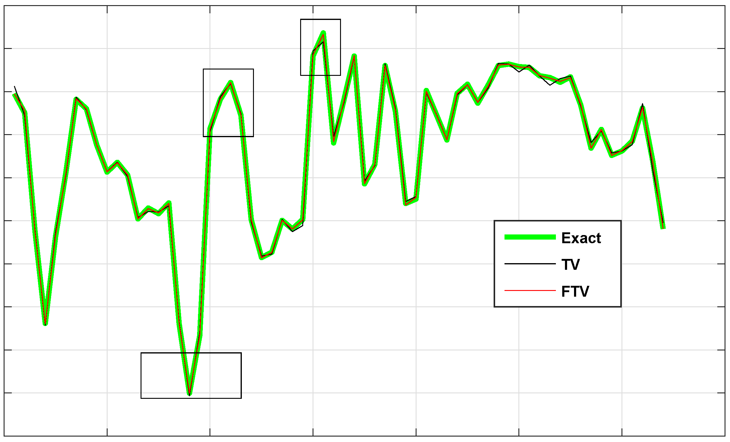
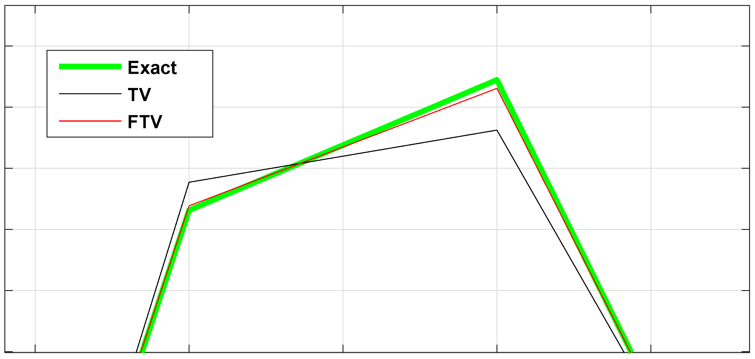
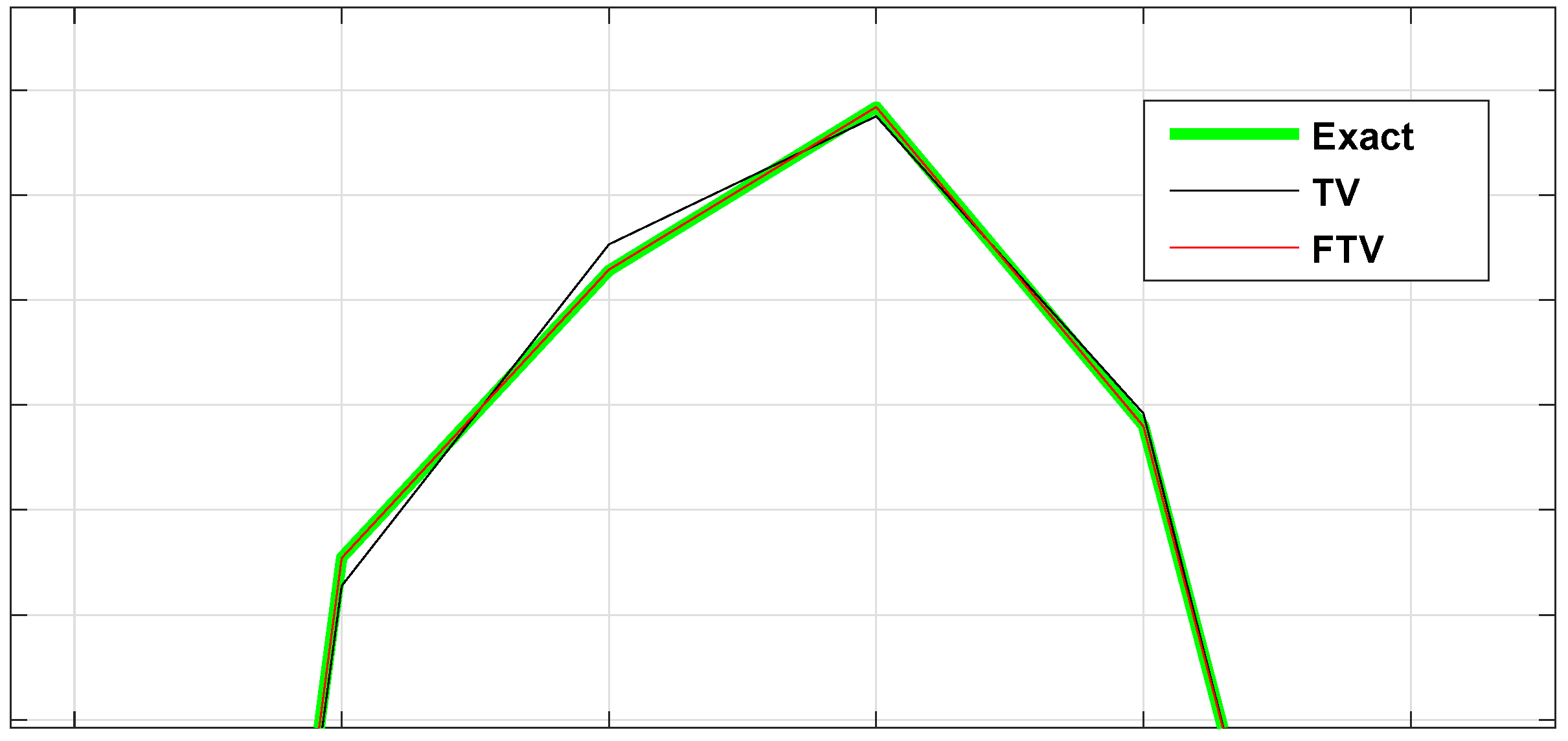
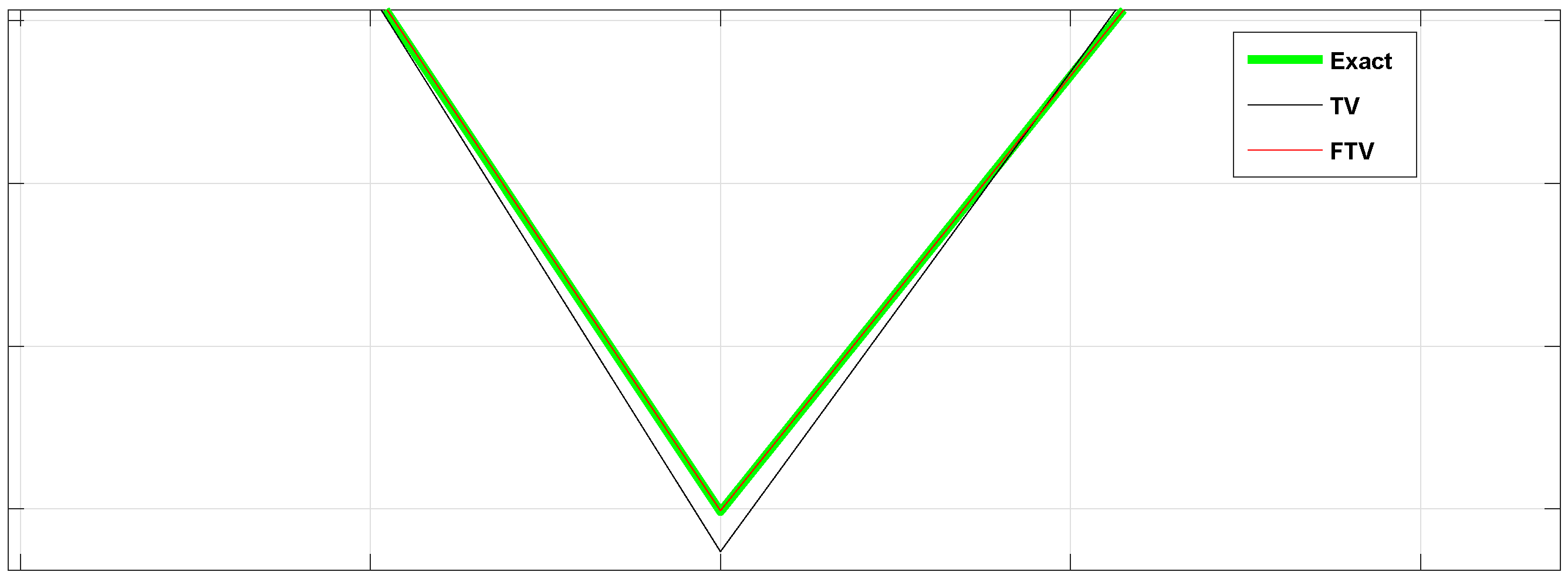
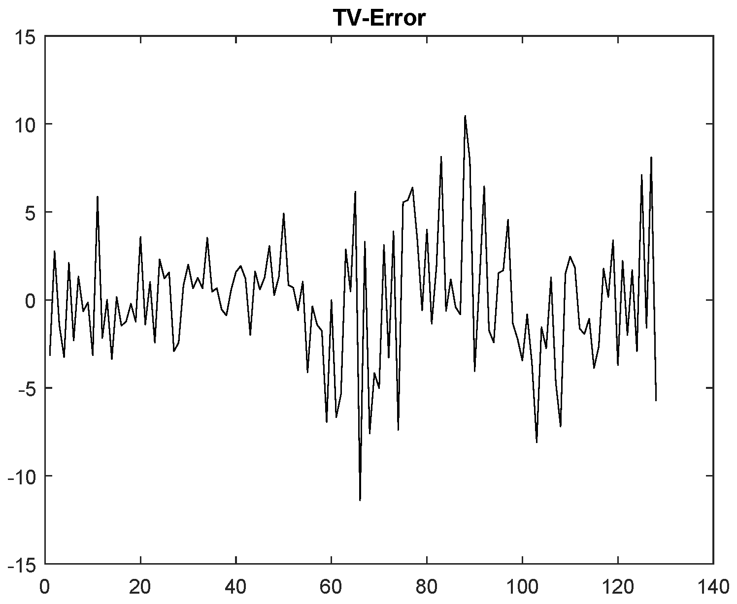
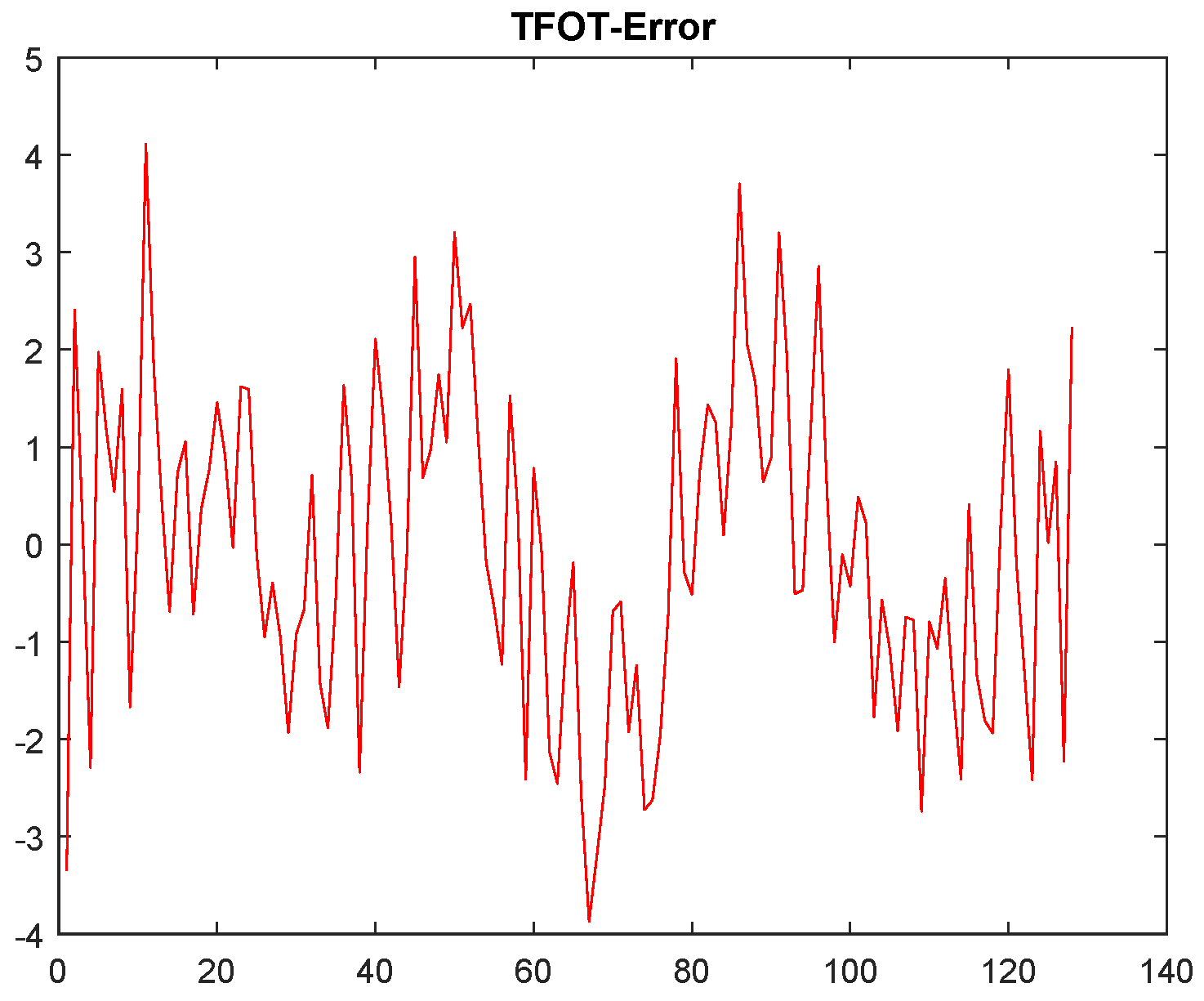
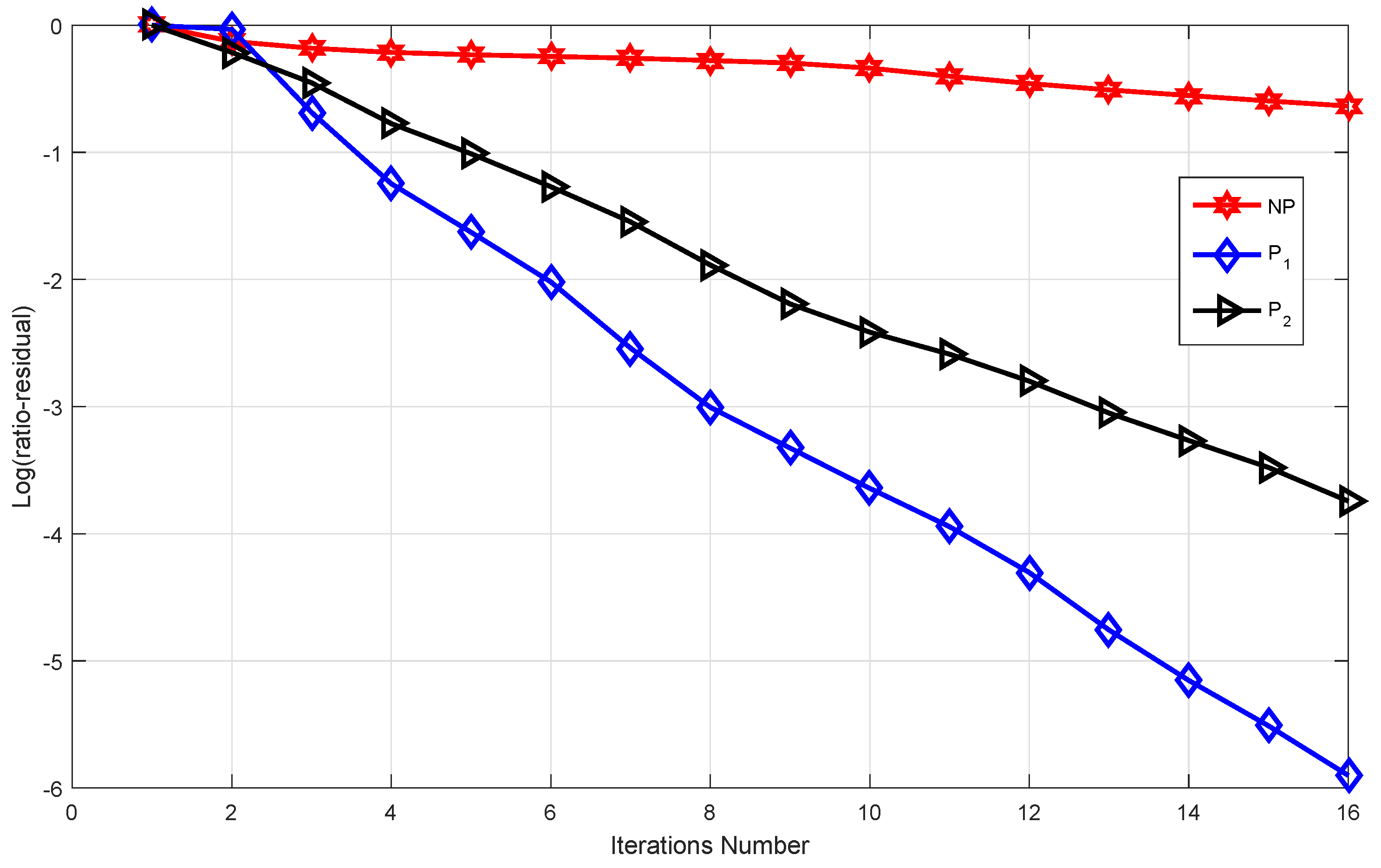
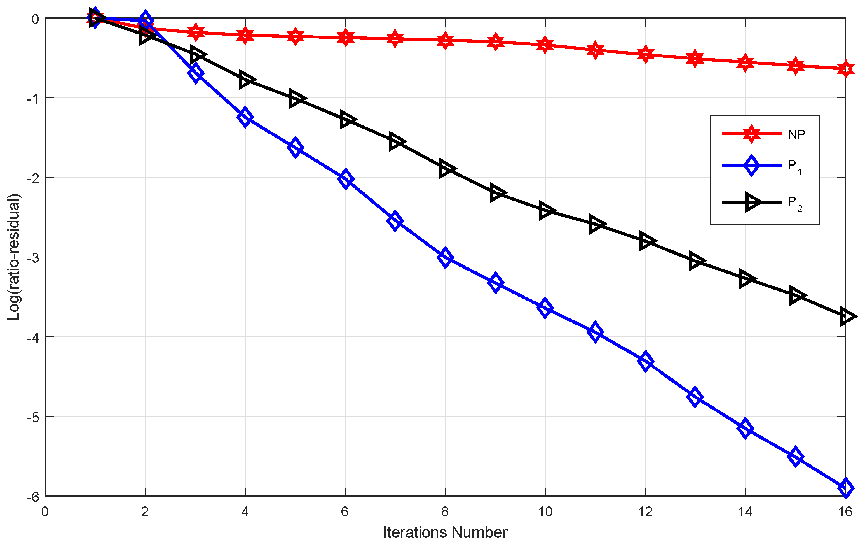
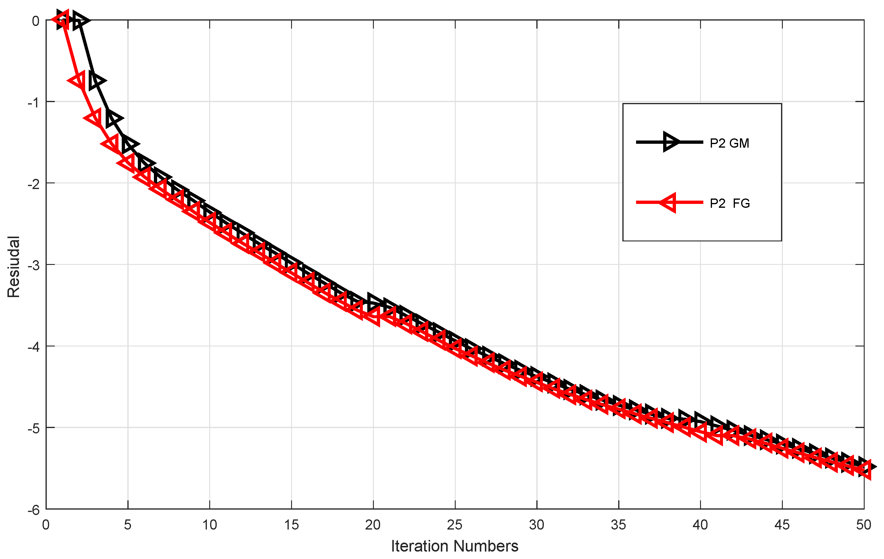
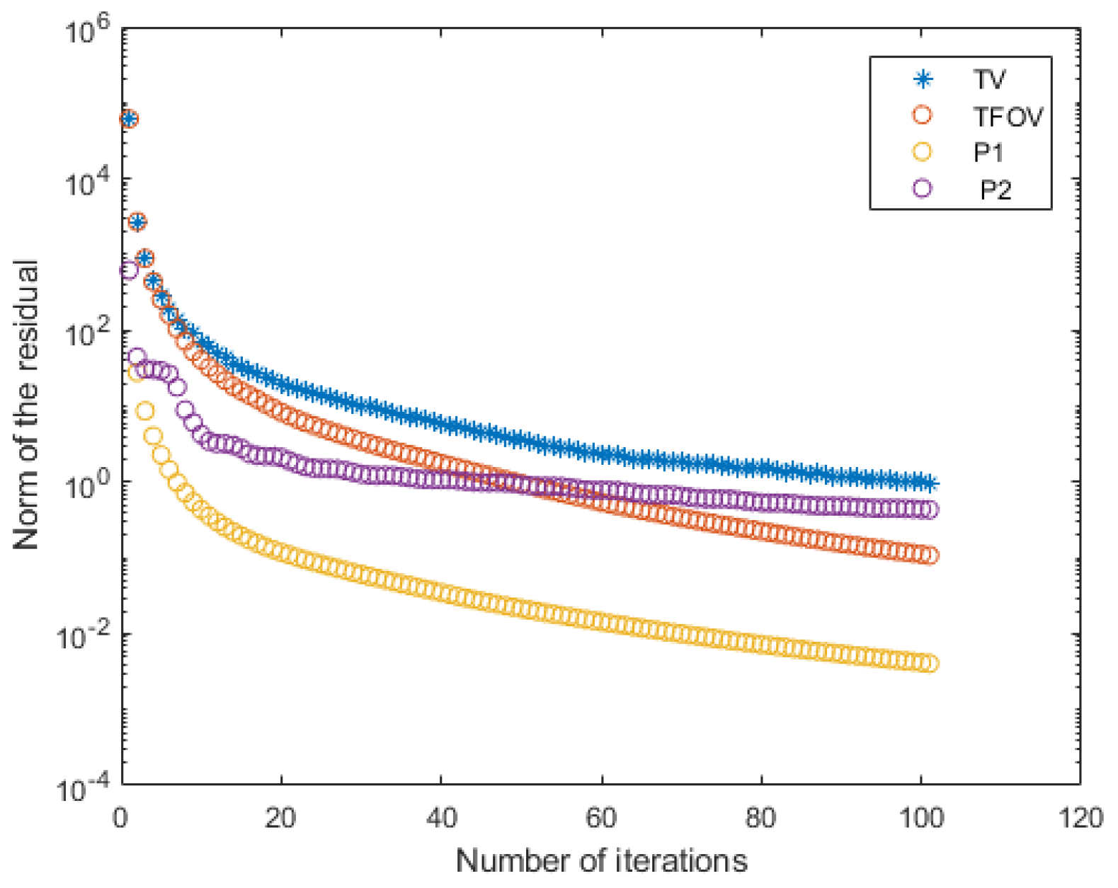
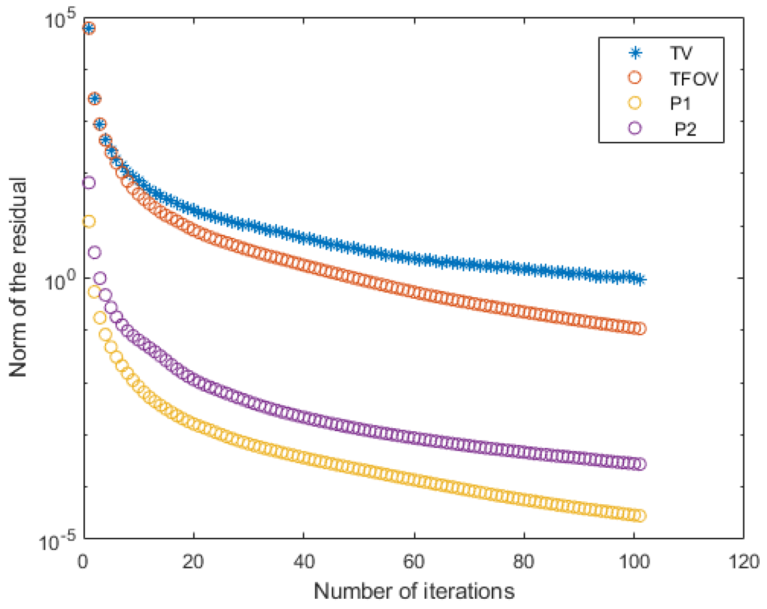
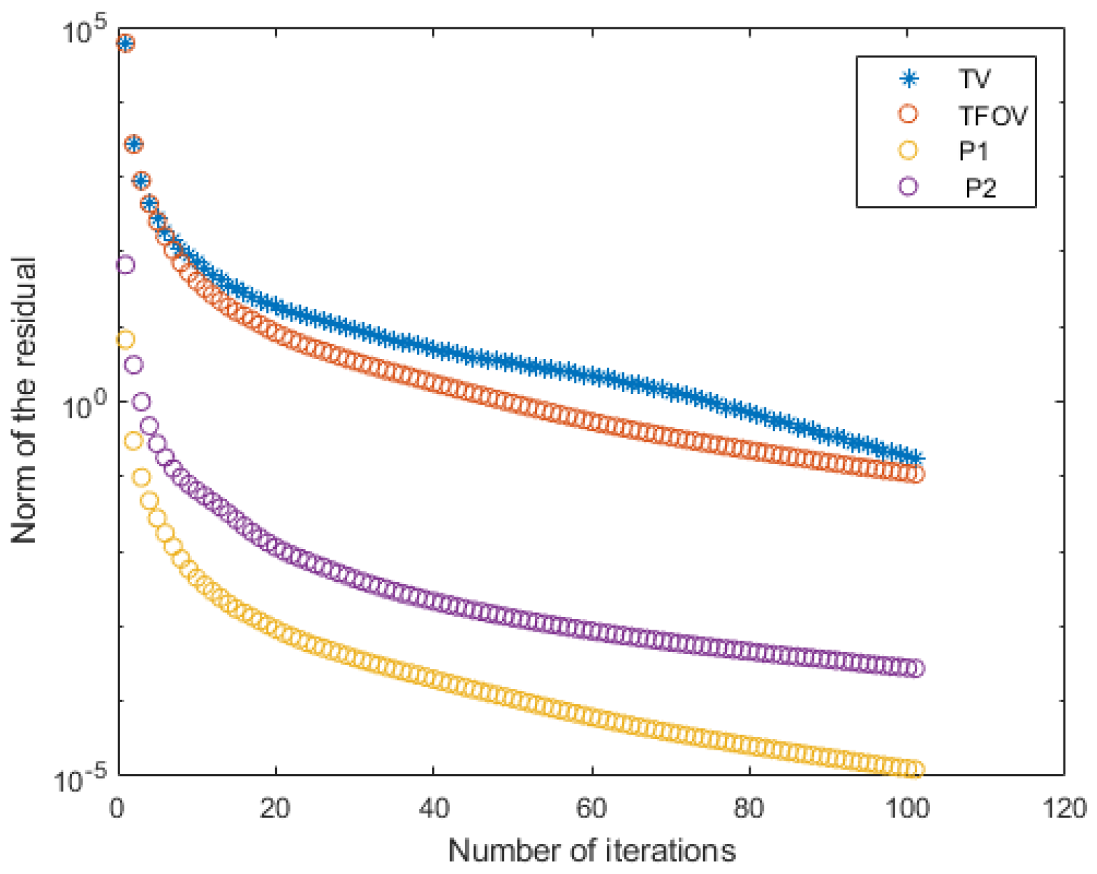
• From Figure 31, Figure 32 and Figure 33, we can clearly see the effectiveness of preconditioning. For all values of N, the number of $P_1$ and $P_2$ iterations is much lower than the number of TFOV-based NP and TV-based $P_1$ iterations to reach the required accuracy $tol={10}^{-7}$. The later fixed-point iterations also have similar results.
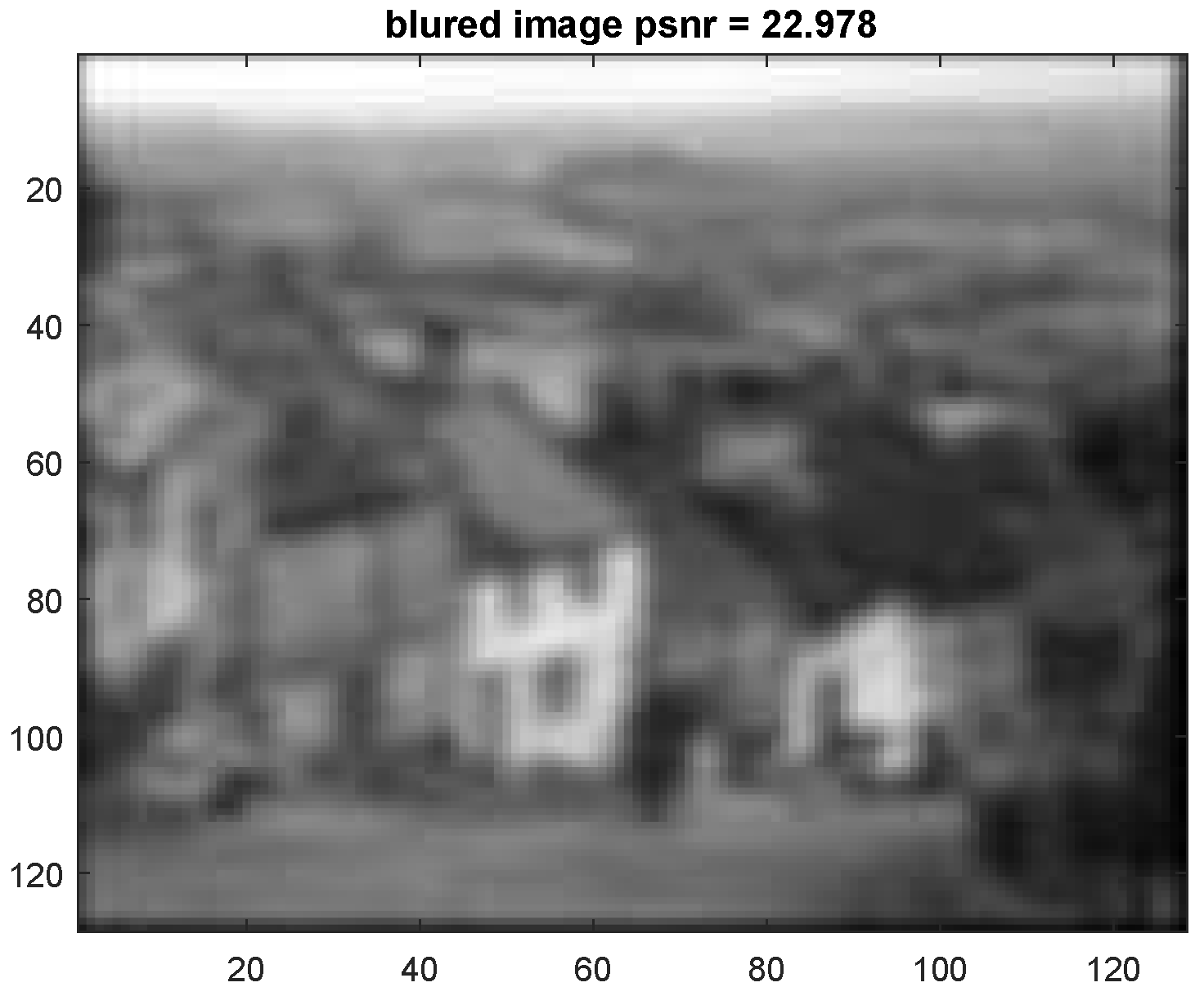
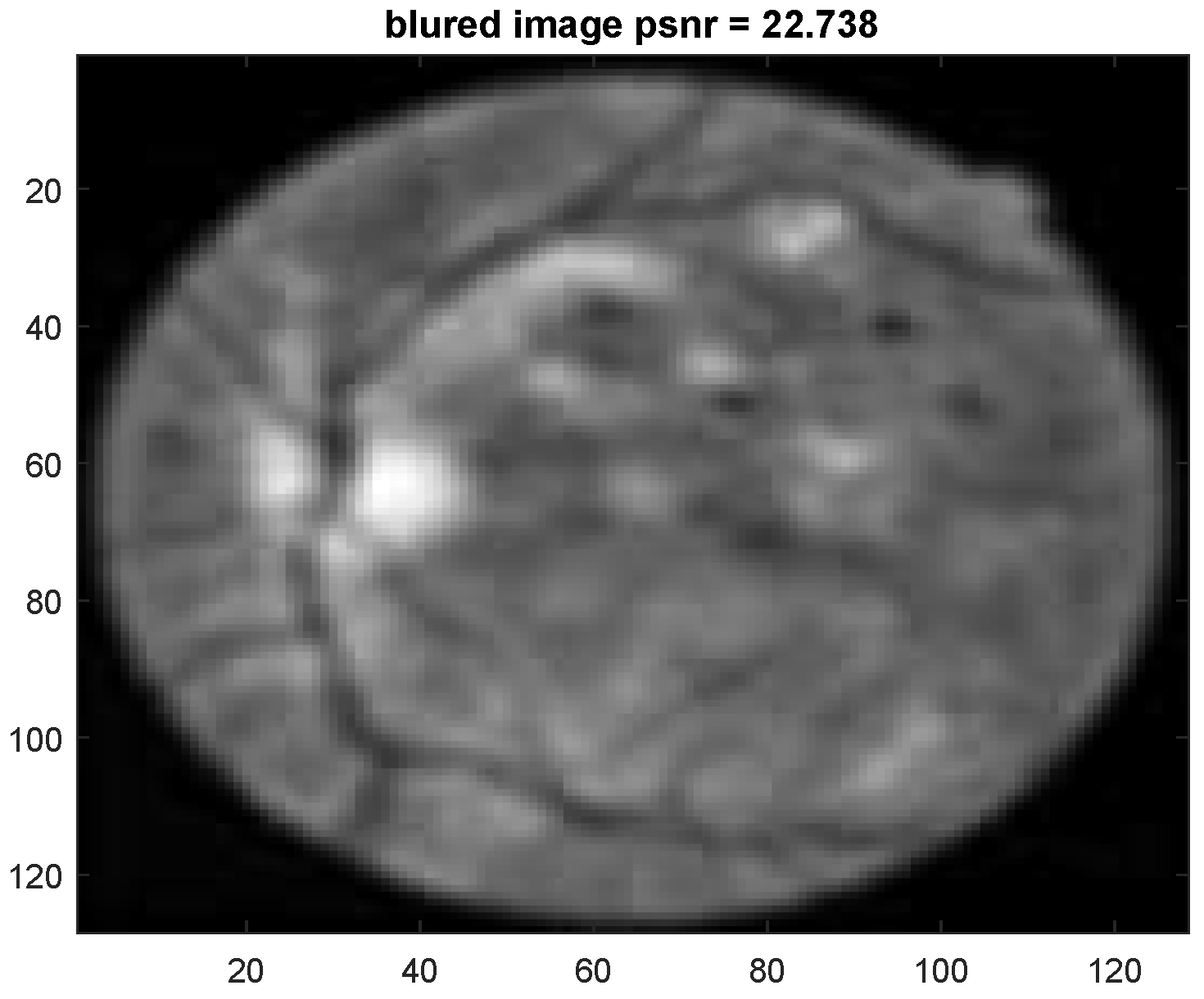
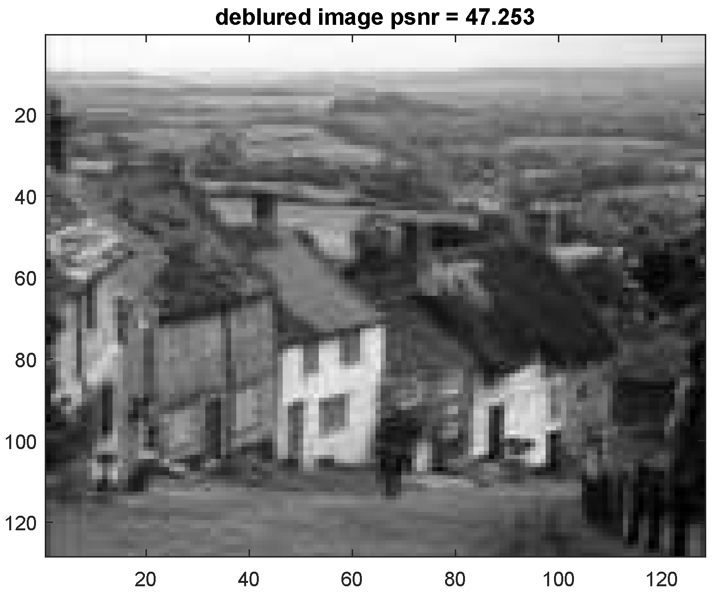
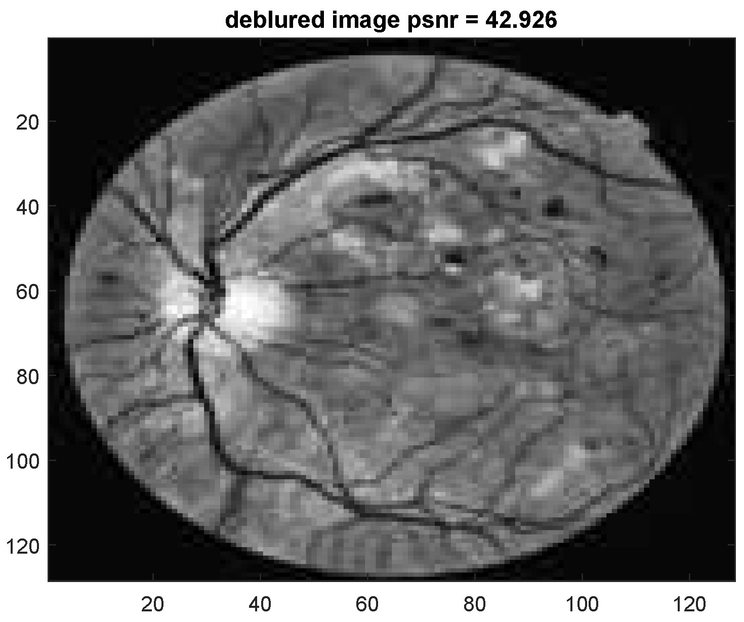
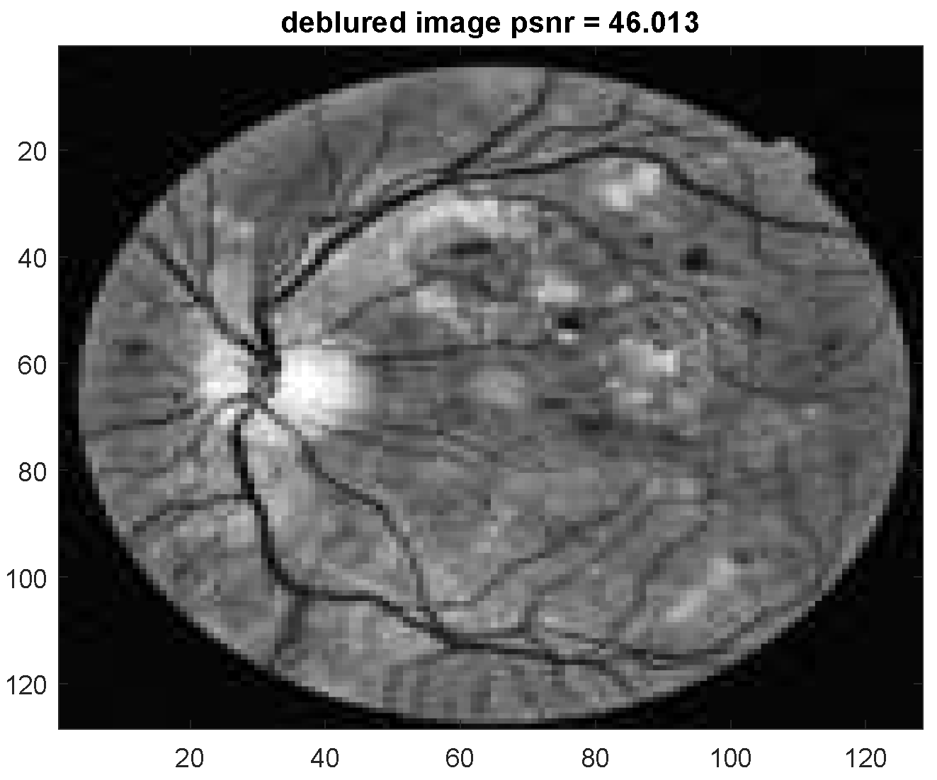
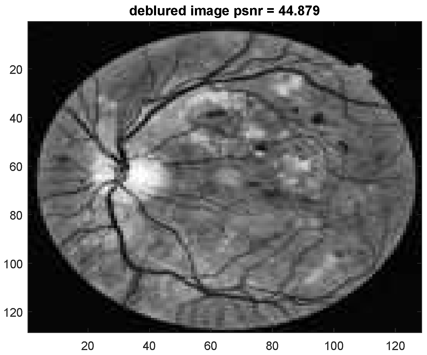
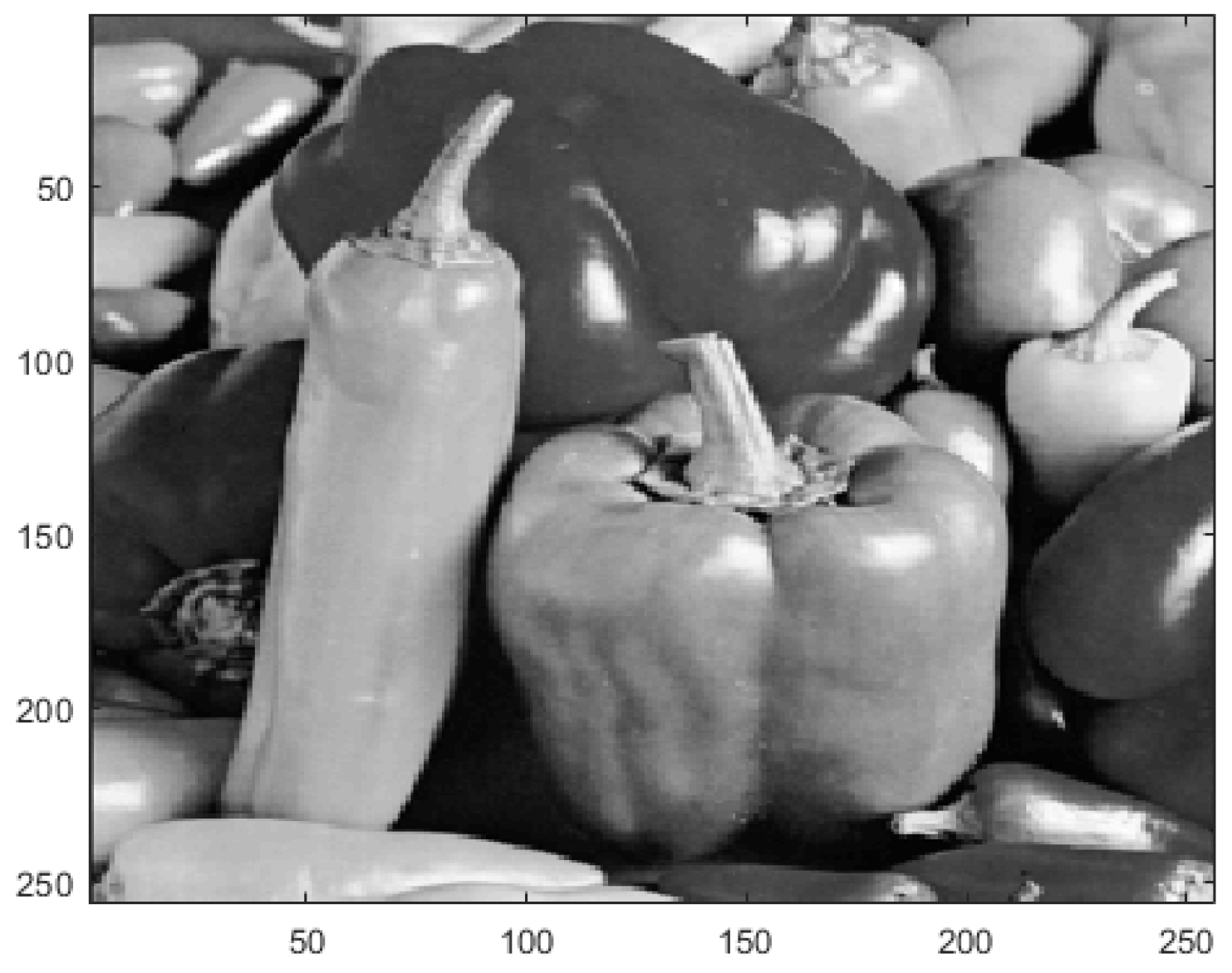
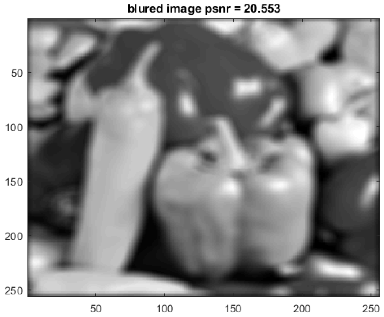
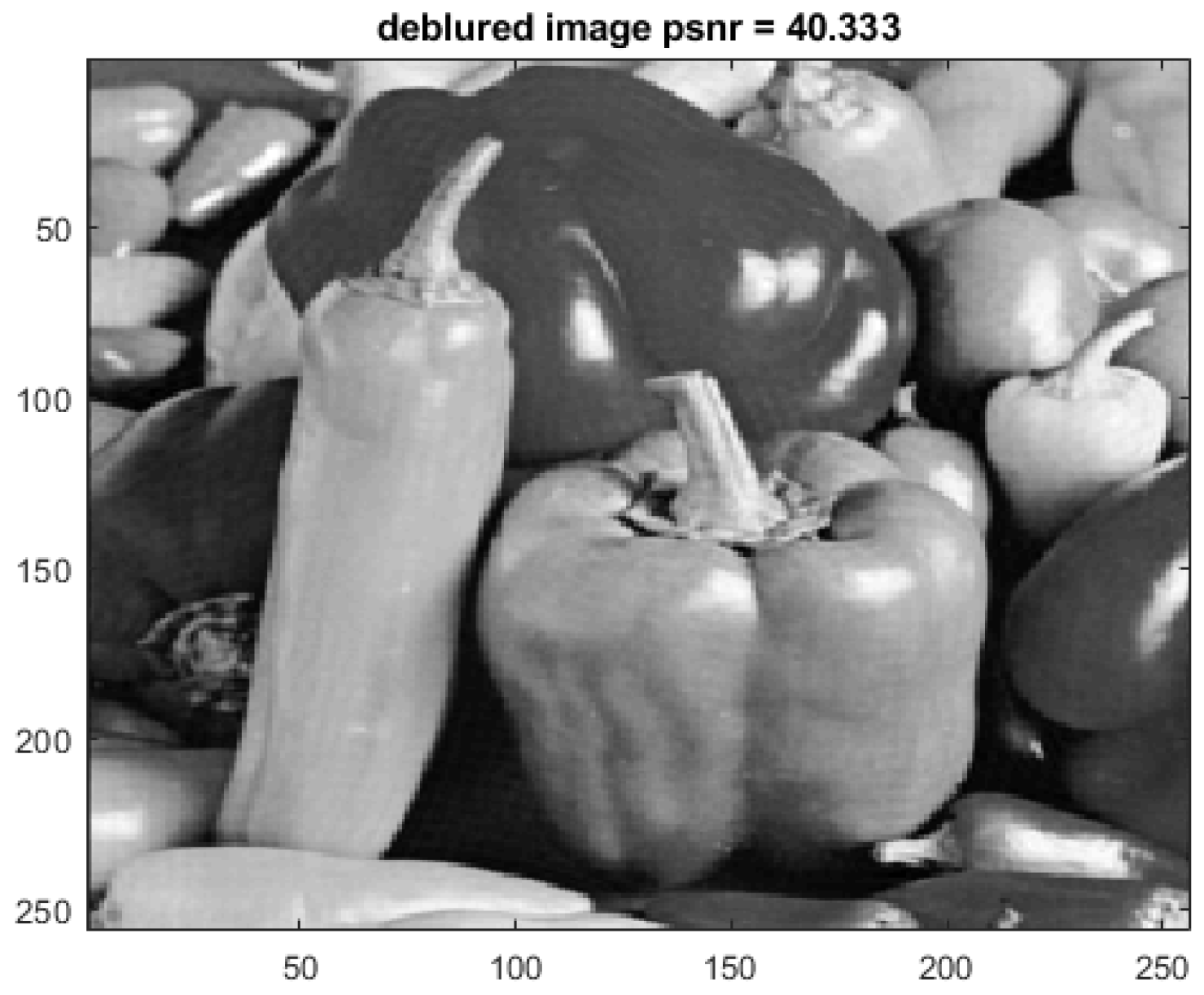
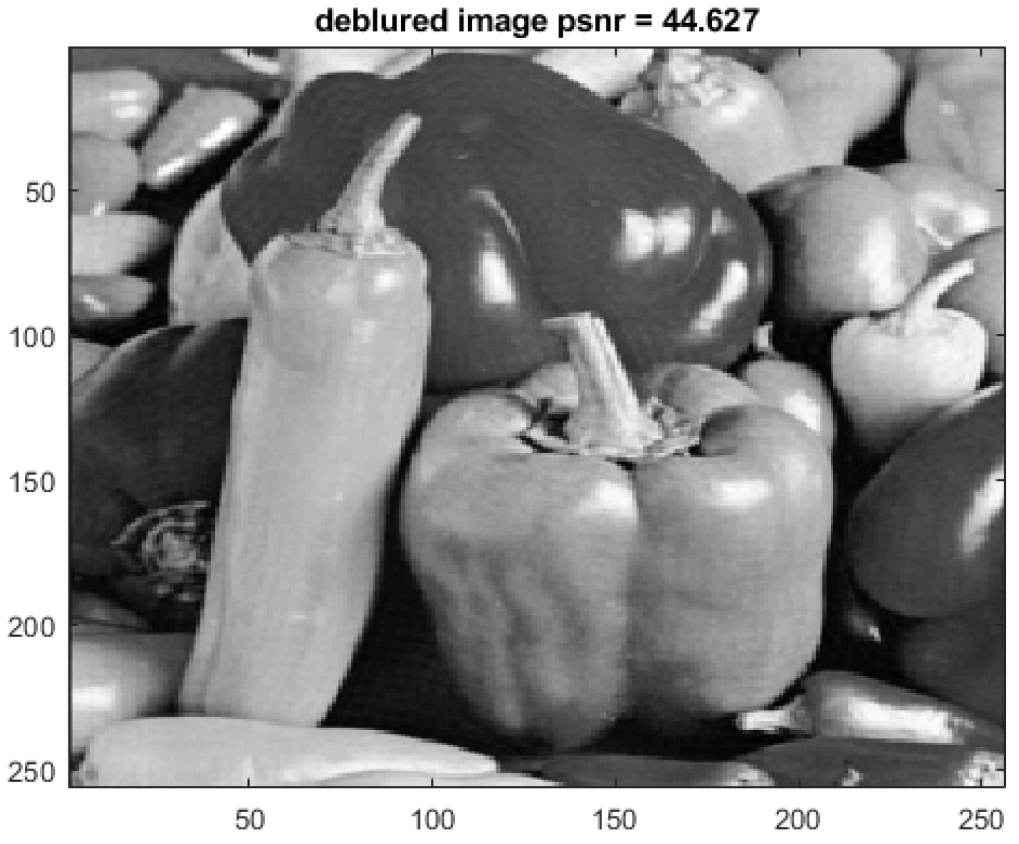
• From Table 2, we observed that the PSNR by the TFOV-based PGMRES method is almost the same as that of the ordinary TFOV-based GMRES method, but much higher than that of the TV-based $P_1$ method for all values of N. However, the $P_1$ and $P_2$ methods generate this better PSNR in much fewer iterations. For example, to achieve a better PSNR the $P_1$ method needs only 18 iterations, and the $P_2$ method needs only 20 iterations for $N=64$. However, the NP method needs 120+ iterations to get the same PSNR. The TV-based $P_1$ method also takes 120+ iterations to get its lower PSNR. The same is the case for other values of N. This means that the TFOV-based FGMRES method is faster than the TFOV-based GMRES and TV-based $P_1$ methods.

Example 7. 

In this example, we utilized satellite images used by Chowdhury et al. [71]. The images underwent deliberate blurring and were corrupted by Poisson noise, resulting in the presence of blurring artifacts. To achieve the blurring, we applied a kernel with specific parameters, namely, we used the Gaussian build in kernel $\text{“}fspecial(\text{‘}gaussian\text{’},9,sqrt\left(3\right))\text{”}$. The introduction of Poisson noise to the image presents a substantial challenge for most deblurring techniques, as this type of noise frequently occurs in scenarios involving photon counting across various imaging methods. Simultaneously, blurring is an inevitable consequence due to the underlying physical principles of the imaging system, which can be thought of as the convolution of the image with a point spread function. For the sake of comparison, we chose to employ the non-blind fractional order TV-based algorithm (NFOV) proposed by Chaudhury et al. [71]. The restored satellite images can be seen in Figure 34, Figure 35, Figure 36, Figure 37 and Figure 38, with each image sized at $128\times 128$. We configured the parameters for the NFOV method as specified in the reference by Chowdhury et al. [71]. For comparison, we have used two different values of N. These are 64 and 128. Their corresponding blurred PSNR are 20.2985 and 20.4559 respectively. The computational technique’s stopping criterion is determined by a tolerance value of $tol={10}^{-7}$. Additional details regarding this experiment can be located in

Table 3. The PSNR Comparison of NFOV, NP, $P_1$ and $P_2$.

Parameters				Iterations				Deblurred PSNR
N	$\alpha$	$\lambda$	$\beta$	NFOV	NP	$P_1$	$P_2$	NFOV	NP	$P_1$	$P_2$
64	1.7	${10}^{-4}$	1	$120+$	$120+$	41	26	25.9869	26.5625	26.7861	26.8283
128	1.9	${10}^{-7}$	1	$120+$	$120+$	65	45	24.1417	25.1908	25.4312	25.6952

.

Remark 2. 

Upon examining Figure 35, Figure 36, Figure 37 and Figure 38 and Table 3, it becomes apparent that the results generated by all methods are virtually indistinguishable. Nevertheless, our proposed methods (GMRES and FGMRES) exhibit slightly higher PSNR values while demanding significantly less CPU time. This observation underscores the improved efficiency and speed of our suggested methods (GMRES and FGMRES) in comparison to the NFOV technique.

6. Conclusions

In this paper we have proposed two block triangular preconditioners for solving the generalized saddle point system which is derived from discretizing the Euler Lagrange equations associated with the TFOV in image de-blurring based problems. We have investigated the performance of the proposed preconditioners with the FGMRES method. We have tested this method on three types of digital images. We have also compared our algorithm with TV based algorithm. Our experiments show that the block triangular preconditioners are very effective. We have also shown that our technique improves the quality of the reconstruction images via calculation of the PSNR. We showed the performance of both GMRES and FGMRES with our proposed preconditioner and we concluded that FGMRES is slightly better than GMRES. Few iterations and CPU-time are needed to obtain a fast rate of convergence and good de-blurring performance. Circulant approximations are used in the first term of the Shur complement to reduce the cost of the computation from $O\left(N^2\right)$ into $O(NlogN)$ and reduce the storage. The spectrums of the preconditioned matrices are clustered around 1 and $-1$.

References

1. Acar, R.; Vogel, C.R. Analysis of bounded variation penalty methods for ill-posed problems. Inverse Probl. 1994, 10, 1217. [Google Scholar] [CrossRef]
2. Agarwal, V.; Gribok, A.V.; Abidi, M.A. Image restoration using L1 norm penalty function. Inverse Probl. Sci. Eng. 2007, 15, 785–809. [Google Scholar] [CrossRef]
3. Aujol, J.-F. Some first-order algorithms for total variation based image restoration. J. Math. Imaging Vis. 2009, 34, 307–327. [Google Scholar] [CrossRef]
4. Tai, X.-C.; Lie, K.-A.; Chan, T.F.; Osher, S. Image processing based on partial differential equations. In Proceedings of the International Conference on PDE-Based Image Processing and Related Inverse Problems, CMA, Oslo, Norway, 8–12 August 2005; Springer Science & Business Media: Berlin/Heidelberg, Germany, 2006. [Google Scholar]
5. Chen, D.; Chen, Y.; Xue, D. Fractional-order total variation image restoration based on primal-dual algorithm. In Abstract and Applied Analysis; Hindawi Publishing Corporation: London, UK, 2013; Volume 2013. [Google Scholar]
6. Williams, B.M.; Zhang, J.; Chen, K. A new image deconvolution method with fractional regularisation. J. Algorithms Comput. 2016, 10, 265–276. [Google Scholar] [CrossRef]
7. Chan, R.; Lanza, A.; Morigi, S.; Sgallari, F. An adaptive strategy for the restoration of textured images using fractional order regularization. Numer. Math. Theory Methods Appl. 2013, 6, 276–296. [Google Scholar] [CrossRef]
8. Zhang, J.; Chen, K. Variational image registration by a total fractional-order variation model. J. Comput. Phys. 2015, 293, 442–461. [Google Scholar] [CrossRef]
9. Benzi, M.; Golub, G.H.; Liesen, J. Numerical solution of saddle point problems. Acta Numer. 2005, 14, 1–137. [Google Scholar] [CrossRef]
10. Silvester, D.; Wathen, A. Fast iterative solution of stabilised Stokes systems. Part II: Using general block preconditioners. SIAM J. Numer. Anal. 1994, 31, 1352–1367. [Google Scholar] [CrossRef]
11. Wathen, A.; Silvester, D. Fast iterative solution of stabilised Stokes systems. Part I: Using simple diagonal preconditioners. SIAM J. Numer. Anal. 1993, 30, 630–649. [Google Scholar] [CrossRef]
12. Bramble, J.H.; Pasciak, J.E. A preconditioning technique for indefinite systems resulting from mixed approximations of elliptic problems. Math. Comput. 1988, 50, 1–17. [Google Scholar] [CrossRef]
13. Cao, Z.-H. Positive stable block triangular preconditioners for symmetric saddle point problems. Appl. Numer. Math. 2007, 57, 899–910. [Google Scholar] [CrossRef]
14. Klawonn, A. Block-triangular preconditioners for saddle point problems with a penalty term. SIAM J. Sci. Comput. 1998, 19, 172–184. [Google Scholar] [CrossRef]
15. Pestana, J. On the eigenvalues and eigenvectors of block triangular preconditioned block matrices. SIAM J. Matrix Anal. Appl. 2014, 35, 517–525. [Google Scholar] [CrossRef]
16. Simoncini, V. Block triangular preconditioners for symmetric saddle-point problems. Appl. Numer. Math. 2004, 49, 63–80. [Google Scholar] [CrossRef]
17. Axelsson, O.; Neytcheva, M. Preconditioning methods for linear systems arising in constrained optimization problems. Numer. Linear Algebr. Appl. 2003, 10, 3–31. [Google Scholar] [CrossRef]
18. Bai, Z.-Z.; Golub, G.H. Accelerated Hermitian and skew-Hermitian splitting iteration methods for saddle-point problems. IMA J. Numer. 2007, 27, 1–23. [Google Scholar] [CrossRef]
19. Benzi, M.; Ng, M.K. Preconditioned iterative methods for weighted Toeplitz least squares problems. SIAM J. Matrix Anal. Appl. 2006, 27, 1106–1124. [Google Scholar] [CrossRef]
20. Ng, M.K.; Pan, J. Weighted Toeplitz regularized least squares computation for image restoration. SIAM J. Sci. Comput. 2014, 36, B94–B121. [Google Scholar] [CrossRef]
21. Cao, Z.-H. Block triangular Schur complement preconditioners for saddle point problems and application to the Oseen equations. Appl. Numer. 2010, 60, 193–207. [Google Scholar] [CrossRef]
22. Chen, C.; Ma, C. A generalized shift-splitting preconditioner for saddle point problems. Appl. Math. Lett. 2015, 43, 49–55. [Google Scholar] [CrossRef]
23. Salkuyeh, D.K.; Masoudi, M.; Hezari, D. On the generalized shift-splitting preconditioner for saddle point problems. Appl. Math. 2015, 48, 55–61. [Google Scholar] [CrossRef]
24. Beik, F.P.A.; Benzi, M.; Chaparpordi, S.-H.A. On block diagonal and block triangular iterative schemes and preconditioners for stabilized saddle point problems. J. Comput. Appl. Math. 2017, 326, 15–30. [Google Scholar] [CrossRef]
25. Murphy, M.F.; Golub, G.H.; Wathen, A.J. A note on preconditioning for indefinite linear systems. Siam J. Sci. Comput. 2000, 21, 1969–1972. [Google Scholar] [CrossRef]
26. Benzi, M.; Golub, G.H. A preconditioner for generalized saddle point problems. SIAM J. Matrix Anal. Appl. 2004, 26, 20–41. [Google Scholar] [CrossRef]
27. Saad, Y. Iterative Methods for Sparse Linear Systems; SIAM: Philadelphia, PA, USA, 2003. [Google Scholar]
28. Vogel, C.R.; Oman, M.E. Fast, robust total variation-based reconstruction of noisy, blurred images. IEEE Trans. Image Process. 1998, 7, 813–824. [Google Scholar] [CrossRef] [PubMed]
29. Axelsson, O. Iterative Solution Methods; Cambridge University Press: Cambridge, UK, 1996. [Google Scholar]
30. Campisi, P.; Egiazarian, K. Blind Image Deconvolution: Theory and Applications; CRC Press: Boca Raton, FL, USA, 2016. [Google Scholar]
31. Groetsch, C.W.; Groetsch, C. Inverse Problems in the Mathematical Sciences; Springer: Berlin/Heidelberg, Germany, 1993; Volume 52. [Google Scholar]
32. Tikhonov, A.N. Regularization of incorrectly posed problems. Sov. Math. Dokl. 1963, 4, 1624–1627. [Google Scholar]
33. Rudin, L.I.; Osher, S.; Fatemi, E. Nonlinear total variation based noise removal algorithms. Phys. D Nonlinear Phenom. 1992, 60, 259–268. [Google Scholar] [CrossRef]
34. Osher, S.; Solé, A.; Vese, L. Image decomposition and restoration using total variation minimization and the h1. Multiscale Model. Simul. 2003, 1, 349–370. [Google Scholar] [CrossRef]
35. Getreuer, P. Total variation inpainting using split Bregman. Image Process. Line 2012, 2, 147–157. [Google Scholar] [CrossRef]
36. Guo, W.; Qiao, L.-H. Inpainting based on total variation. In Proceedings of the 2007 International Conference on Wavelet Analysis and Pattern Recognition, Beijing, China, 2–4 November 2007; Volume 2, pp. 939–943. [Google Scholar]
37. Bresson, X.; Esedoglu, S.; Vandergheynst, P.; Thiran, J.-P.; Osher, S. Fast global minimization of the active contour/snake model. J. Math. Imaging Vis. 2007, 28, 151–167. [Google Scholar] [CrossRef]
38. Unger, M.; Pock, T.; Trobin, W.; Cremers, D.; Bischof, H. Tvseg-interactive total variation based image segmentation. BMVC 2008, 31, 44–46. [Google Scholar]
39. Yan, H.; Zhang, J.-X.; Zhang, X. Injected infrared and visible image fusion via l_{1} decomposition model and guided filtering. IEEE Trans. Comput. Imaging 2022, 8, 162–173. [Google Scholar] [CrossRef]
40. Chan, T.; Marquina, A.; Mulet, P. High-order total variation-based image restoration. SIAM J. Sci. Comput. 2000, 22, 503–516. [Google Scholar] [CrossRef]
41. Steidl, G.; Didas, S.; Neumann, J. Relations between higher order TV regularization and support vector regression. In International Conference on Scale-Space Theories in Computer Vision; Springer: Berlin/Heidelberg, Germany, 2005; pp. 515–527. [Google Scholar]
42. Bredies, K.; Kunisch, K.; Pock, T. Total generalized variation. SIAM J. Imaging Sci. 2010, 3, 492–526. [Google Scholar] [CrossRef]
43. Zhu, W.; Chan, T. Image denoising using mean curvature of image surface. SIAM J. Imaging Sci. 2012, 5, 1–32. [Google Scholar] [CrossRef]
44. Lysaker, M.; Osher, S.; Tai, X.-C. Noise removal using smoothed normals and surface fitting. IEEE Trans. Image Process. 2004, 13, 1345–1357. [Google Scholar] [CrossRef]
45. Ahmad, S.; Al-Mahdi, A.M.; Ahmed, R. Two new preconditioners for mean curvature-based image deblurring problem. AIMS Math. 2021, 6, 13824–13844. [Google Scholar] [CrossRef]
46. Al-Mahdi, A.; Fairag, F. Block diagonal preconditioners for an image de-blurring problem with fractional total variation. J. Phys. Conf. Ser. 2018, 1132, 012063. [Google Scholar] [CrossRef]
47. Fairag, F.; Al-Mahdi, A.; Ahmad, S. Two-level method for the total fractional-order variation model in image deblurring problem. Numer. Algorithms 2020, 85, 931–950. [Google Scholar] [CrossRef]
48. Sohail, A.; Bég, O.; Li, Z.; Celik, S. Physics of fractional imaging in biomedicine. Prog. Biophys. Mol. Biol. 2018, 140, 13–20. [Google Scholar] [CrossRef]
49. Xu, K.-D.; Zhang, J.-X. Prescribed performance tracking control of lower-triangular systems with unknown fractional powers. Fractal Fract. 2023, 7, 594. [Google Scholar] [CrossRef]
50. Wang, Y.; Zhang, X.; Boutat, D.; Shi, P. Quadratic admissibility for a class of lti uncertain singular fractional-order systems with 0 < α < 2. Fractal Fract. 2022, 7, 1. [Google Scholar]
51. Zhang, J.; Chen, K. A total fractional-order variation model for image restoration with nonhomogeneous boundary conditions and its numerical solution. SIAM J. Imaging Sci. 2015, 8, 2487–2518. [Google Scholar] [CrossRef]
52. Miller, K.S.; Ross, B. An Introduction to the Fractional Calculus and Fractional Differential Equations; Wiley: Hoboken, NJ, USA, 1993. [Google Scholar]
53. Oldham, K.; Spanier, J. The Fractional Calculus Theory and Applications of Differentiation and Integration to Arbitrary Order; Elsevier: Amsterdam, The Netherlands, 1974; Volume 111. [Google Scholar]
54. Podlubny, I. Fractional Differential Equations: An Introduction to Fractional Derivatives, Fractional Differential Equations, to Methods of Their Solution and Some of Their Applications; Academic Press: Cambridge, MA, USA, 1998; Volume 198. [Google Scholar]
55. Chan, T.F.; Golub, G.H.; Mulet, P. A nonlinear primal-dual method for total variation-based image restoration. SIAM J. Sci. 1999, 20, 1964–1977. [Google Scholar] [CrossRef]
56. Meerschaert, M.M.; Tadjeran, C. Finite difference approximations for fractional advection–dispersion flow equations. J. Comput. Appl. Math. 2004, 172, 65–77. [Google Scholar] [CrossRef]
57. Meerschaert, M.M.; Tadjeran, C. Finite difference approximations for two-sided space-fractional partial differential equations. Appl. Numer. Math. 2006, 56, 80–90. [Google Scholar] [CrossRef]
58. Wang, H.; Du, N. Fast solution methods for space-fractional diffusion equations. J. Comput. Appl. Math. 2014, 255, 376–383. [Google Scholar] [CrossRef]
59. Strang, G. A proposal for Toeplitz matrix calculations. Stud. Appl. Math. 1986, 74, 171–176. [Google Scholar] [CrossRef]
60. Olkin, J.A. Linear and Nonlinear Deconvolution Problems (Optimization). Ph.D. Thesis, Rice University, Houston, TX, USA, 1986. [Google Scholar]
61. Chan, T.F.; Olkin, J.A. Circulant preconditioners for Toeplitz-block matrices. Numer. Algorithms 1994, 6, 89–101. [Google Scholar] [CrossRef]
62. Chan, R.H.; Ng, K.-P. Toeplitz preconditioners for Hermitian Toeplitz systems. Linear Algebra Appl. 1993, 190, 181–208. [Google Scholar] [CrossRef]
63. Lin, F.-R. Preconditioners for block Toeplitz systems based on circulant preconditioners. Numer. Algorithms 2001, 26, 365–379. [Google Scholar] [CrossRef]
64. Chan, R.H. Toeplitz preconditioners for Toeplitz systems with nonnegative generating functions. IMA J. Numer. Anal. 1991, 11, 333–345. [Google Scholar] [CrossRef]
65. Serra, S. Preconditioning strategies for asymptotically ill-conditioned block Toeplitz systems. BIT Numer. Math. 1994, 34, 579–594. [Google Scholar] [CrossRef]
66. Lin, F.-R.; Wang, C.-X. BTTB preconditioners for BTTB systems. Numer. Algorithms 2012, 60, 153–167. [Google Scholar] [CrossRef]
67. Chan, R.H.; Strang, G. Toeplitz equations by conjugate gradients with circulant preconditioner. SIAM J. Sci. Stat. 1989, 10, 104–119. [Google Scholar] [CrossRef]
68. Chan, R.H.; Yeung, M.-C. Circulant preconditioners constructed from kernels. SIAM J. Numer. Anal. 1992, 29, 1093–1103. [Google Scholar] [CrossRef]
69. Chan, T.F. An optimal circulant preconditioner for Toeplitz systems. SIAM J. Sci. Stat. Comput. 1988, 9, 766–771. [Google Scholar] [CrossRef]
70. Davis, P.J. Circulant Matrices; American Mathematical Soc.: New York, NY, USA, 2012. [Google Scholar]
71. Chowdhury, M.R.; Qin, J.; Lou, Y. Non-blind and blind deconvolution under Poisson noise using fractional-order total variation. J. Math. Imaging Vis. 2020, 62, 1238–1255. [Google Scholar] [CrossRef]
Figure 1. Cross sections.
Mca 28 00097 g001
Figure 2. Right box.
Mca 28 00097 g002
Figure 3. Middle box.
Mca 28 00097 g003
Figure 4. Left box.
Mca 28 00097 g004
Figure 5. TV-error.
Mca 28 00097 g005
Figure 6. TFOV-error.
Mca 28 00097 g006
Figure 7. Eigenvalues of A.
Mca 28 00097 g007
Figure 8. Eigenvalues of ( P 1 ) 1 A .
Mca 28 00097 g008
Figure 9. Golden house image.
Mca 28 00097 g009
Figure 10. Retinal image.
Mca 28 00097 g010
Figure 11. Shape of the kernel.
Mca 28 00097 g011
Figure 12. Residual versus iterations number when λ = 1 × 10 3 .
Mca 28 00097 g012
Figure 13. Residual versus iterations number when λ = 1 × 10 5 .
Mca 28 00097 g013
Figure 14. Golden house image (blurred).
Mca 28 00097 g014
Figure 15. Retinal image (blurred).
Mca 28 00097 g015
Figure 16. Using P 1 with α = 1 .
Mca 28 00097 g016
Figure 17. Using P 2 with α = 1 .
Mca 28 00097 g017
Figure 18. Using P 1 with α = 1.8 .
Mca 28 00097 g018
Figure 19. Using P 2 with α = 1.8 .
Mca 28 00097 g019
Figure 20. Using P 1 with α = 1 .
Mca 28 00097 g020
Figure 21. Using P 2 with α = 1 .
Mca 28 00097 g021
Figure 22. Using P 1 with α = 1.8 .
Mca 28 00097 g022
Figure 23. Using P 2 with α = 1.8 .
Mca 28 00097 g023
Figure 24. FGMRES vs. GMRES.
Mca 28 00097 g024
Figure 25. Peppers image (exact).
Mca 28 00097 g025
Figure 26. Peppers image (blurred).
Mca 28 00097 g026
Figure 27. Using TV ( α = 1 ).
Mca 28 00097 g027
Figure 28. Using NP.
Mca 28 00097 g028
Figure 29. Using P 1 with α = 1.9 .
Mca 28 00097 g029
Figure 30. Using P 2 with α = 1.9 .
Mca 28 00097 g030
Figure 31. N = 64 .
Mca 28 00097 g031
Figure 32. N = 128 .
Mca 28 00097 g032
Figure 33. N = 256 .
Mca 28 00097 g033
Figure 34. Satel image (blurred).
Mca 28 00097 g034
Figure 35. Using NFOV.
Mca 28 00097 g035
Figure 36. Using NP.
Mca 28 00097 g036
Figure 37. Using P 1 with α = 1.9 .
Mca 28 00097 g037
Figure 38. Using P 2 with α = 1.9 .
Mca 28 00097 g038