New Quality Measures for Quadrilaterals and New Discrete Functionals for Grid Generation

Abstract

In this paper, we review some grid quality metrics and define some new quality measures for quadrilateral elements. The curved elements are not discussed. Usually, the maximum value of a quality measure corresponds to the minimum value of the energy density over the grid. We also define new discrete functionals, which are implemented as objective functions in an optimization-based method for quadrilateral grid generation and improvement. These functionals are linearly combined with a discrete functional whose domain has an infinite barrier at the boundary of the set of unfolded grids to preserve convex grid cells in each step of the optimization process.

1. Introduction

Research on mesh generation in Computer Graphics, Scientific Visualization and Computational Field Simulations has led to a substantial number of methods within the last six decades. An exhaustive description of this field is beyond the scope of this paper; one can refer to the many surveys available, see, e.g., Thompson et al. [1] and Lo [2]. However, that mesh generation in regions in 2D and 3D is a central task, used in numerical methods for the solution of partial differential equations, using finite difference, finite element and finite volume methods.

There is also a special interest in studying meshes formed by triangular elements. Our interest here is to generate structured meshes with quadrilateral elements; however, all of the discussion can be applied to unstructured meshes. The simplest way to generate a structured mesh is via interpolation of the boundaries, but it is difficult to ensure that the mesh thus obtained is a convex one. In 2010, Barrera et al. [3] provided a review of some functionals and conditions that guarantee the existence of optimal meshes that are convex over irregular planar regions.

Our interest now is to improve the mesh quality via controlling the shape of the elements. The improvement of mesh quality can be carried out in two ways:

Clean-up. 

This consists of the elimination, insertion and reconnection of nodes to eliminate the worst elements. Some authors call that this procedure topological optimization in the sense that the connectivity of the nodes is removed to obtain an optimal configuration.

Smoothing.

This consists of node repositioning without changing the connectivity of the elements.

In both cases, the goal is to obtain a quality mesh with a low number of distorted elements. To achieve this goal for a quadrilateral, it is neccesary to define an ad hoc quality measure.

Definition 1

(González [4]). We say that a real-valued function $\mu \left(Q\right)$ over a quadrilateral Q is a quality measure in the sense of Field-Oddy if it

(1) 

Has the ability to detect degenerated elements;

(2) 

Is bounded and continuous;

(3) 

Is independent of scale;

(4) 

Is normalized;

(5) 

Is invariant under rigid transformations.

For practical purposes, it is convenient to define an acceptability interval $[{\mu }_0,1]$ for the quality measure, i.e., when a quadrilateral has a suitable shape, outside of this interval, we say that the quadrilateral does not have the desired shape. The acceptability interval are defined empirically for each quality measure.

In this paper, we are interested in identifying the shape of the cells and in quantifying the distortion of a quadrilateral when it is not a square or a rectangle. In the remainder of this paper, we will discuss the most used quality measures for rectangles and then propose new quality measures.

The remainder of this paper is structured as follows. The following, background section presents the most used quality measures for rectangles based on angles. Section 3 then presents some new quality measures based on geometric properties. Section 4 then presents some classical global quality metrics and proposes a statistical analysis of all elements of the mesh. Section 5 then presents some concepts to grid quality improvement using quality measures. Finally in the Section 6 then presents some new quality discrete functionals for improvement of the mesh.

2. Background

Following the ideas behind the quality measures for triangles, it is straightforward to define some figures that measure the shape of quadrilaterals. One of these is the aspect ratio, which is defined by comparing to the ideal case when the quadrilateral is a rectangle; it represents the ratio of the largest to the smallest sides. An estimator for this ratio was discussed in 1987 by Robinson [5]. The idea is to associate a rectangle with the convex quadrilateral: a rectangle passing through the midpoints of the sides of the quadrilateral, see Figure 1.

This idea is usual in continuum mechanics. Robinson proposed a practical method of calculating it by means of bilinear mapping between the unit square and the quadrilateral

$$\begin{array}{ccc}\hfill x& =& e_1+e_2\xi +e_3\eta +e_4\xi \eta ,\hfill \end{array}$$

(1)

$$\begin{array}{ccc}\hfill y& =& f_1+f_2\xi +f_3\eta +f_4\xi \eta ,\hfill \end{array}$$

(2)

where the e and f coefficients are realated to the nodal coordinates $x_1$ to $x_4$ and $y_1$ to $y_4$ by

$$\begin{array}{ccccccc}\hfill e_1& =& \frac{1}{4}(x_1+x_2+x_3+x_4)\hfill & & \hfill e_2& =& \frac{1}{4}(-x_1+x_2+x_3-x_4)\hfill \\ \hfill e_3& =& \frac{1}{4}(-x_1-x_2+x_3+x_4)\hfill & & \hfill e_4& =& \frac{1}{4}(x_1-x_2+x_3-x_4)\hfill \\ \hfill f_1& =& \frac{1}{4}(y_1+y_2+y_3+y_4)\hfill & & \hfill f_2& =& \frac{1}{4}(-y_1+y_2+y_3-y_4)\hfill \\ \hfill f_3& =& \frac{1}{4}(-y_1-y_2+y_3+y_4)\hfill & & \hfill f_4& =& \frac{1}{4}(y_1-y_2+y_3-y_4)\hfill \end{array}$$

(3)

The meaning of the coefficients in Equation (3) is now shown in [5]. Which yields

$$\mathrm{a}\mathrm{s}\mathrm{p}\mathrm{e}\mathrm{c}\mathrm{t}\mathrm{r}\mathrm{a}\mathrm{t}\mathrm{i}\mathrm{o}=max\left\{\frac{e_2}{f_3},\frac{f_3}{e_2}\right\}.$$

The associated rectangle has sides, which are parallel to the coordinate axes and pass through the midpoints of the sides of the quadrilateral. In spite of its simplicity, this analytic representation is not satisfactory since it depends on an orthogonal coordinate system. In 2000, Field [6] reviewed this definition and suggested calculating the aspect ratio of Robinson and orthogonalizing the main axes, and proposed a quality measure to detect squares.

In 1989, Lo [7] reviewed the classical quality measure for triangles $T(a,b,c)$ with side lengths $l_1$, $l_2$ and $l_3$,

$$g_i=4\sqrt{3}\frac{\text{area}\left(T_i\right)}{l_1^2+l_2^2+l_3^2}$$

(4)

which attains its optimum value in equilateral triangles, and again proposed calculating each one of those values over the four $T_i$ triangles, which are defined by the sides and diagonals of a quadrilateral, but reordering these quantities in such a way that

$$g_1\le g_2\le g_3\le g_4,$$

(5)

and using

$$\mu 1\left(Q\right)=\frac{g_1{g}_2}{g_3{g}_4},$$

(6)

as a quality measure. The maximum value is 1 and it is obtained for rectangles. This is a quality measure because it is continuous, bounded and identifies degenerate and even non-convex quadrilaterals. The measure that Lo uses for triangles T is the reciprocal of the number of conditions of a linear mapping $\mu \left(T\right)=1/{\kappa }_2\left(T\right)$, which Knupp [8] used in 2001 to measure the distortion of the elements. Locally, Lo’s measure may have more critical points, which can be far from representing a rectangle.

Another measure of quality for quadrilaterals is described by van Rens et al. [9] as follows: compute the inner angles ${\theta }_k$ and define

$${\mu }_2\left(Q\right)=\prod _{k=1}^4\left(1-\left|\frac{\frac{\pi }{2}-{\theta }_k}{\frac{\pi }{2}}\right|\right).$$

(7)

This function is continuous, dimensionless and $0\le {\mu }_2\left(Q\right)\le 1$. One can see that ${\mu }_2\left(Q\right)=0$ if Q is a triangle and ${\mu }_2\left(Q\right)=1$ only if Q is a rectangle.

In 2012, Remacle et al. [10] described the Blossom-Quad algorithm to construct a non-structured mesh with quadrilateral elements obtained from a previous triangulation and used a cost function to produce a quality mesh. They used

$${\mu }_3\left(Q\right)=max\left\{1-\frac{2}{\pi }\underset{k}{max}\left\{|\frac{\pi }{2}-{\theta }_k|\right\},0\right\},$$

(8)

and observed that if the value of this function is 1, Q is a perfect quadrilateral, and it is 0 if any of the angles are greater than or equal to $\pi$, i.e., when the quadrilateral degenerates into a triangle or is nonconvex. This function is also a quality measure.

As noted, unlike other measures for rectangles we have discussed up to this point, the last two ones do not depend either on the shape of the quadrilaterals or the aspect ratio or proportion of their sides; they only measure how near or far away a quadrilateral is from being a rectangle using only the internal angles.

Another function based on the inner angles was proposed by Wu [11]. This author used the same idea as Lo: to order the inner angles ${\theta }_i$ so that ${\theta }_1\le {\theta }_2\le {\theta }_3\le {\theta }_4$ and define

$${\mu }_4\left(Q\right)=\frac{{\theta }_1{\theta }_2}{{\theta }_3{\theta }_4}.$$

(9)

This function reaches its maximum value of 1 on rectangles. However, this is not a good measure in the sense of Field-Oddy, since it is not capable of detecting degenerate quadrilaterals.

3. New Quality Measures

In the previous section, we had reviewed some measures that characterize rectangles and also pointed out some intervals of acceptability to decide if a quadrilateral is close to the desired shape. However, which rectangle is it close to?

3.1. Quality Measure of Rectangles

A very interesting problem in computational geometry is the following: given a cloud of points, calculate the rectangle of the minimum area that contains them. It is known that this problem can be raised directly on the convex hull of the cloud of points, and therefore the problem can be regarded as calculating a rectangle of minimum area that contains a convex polygon.

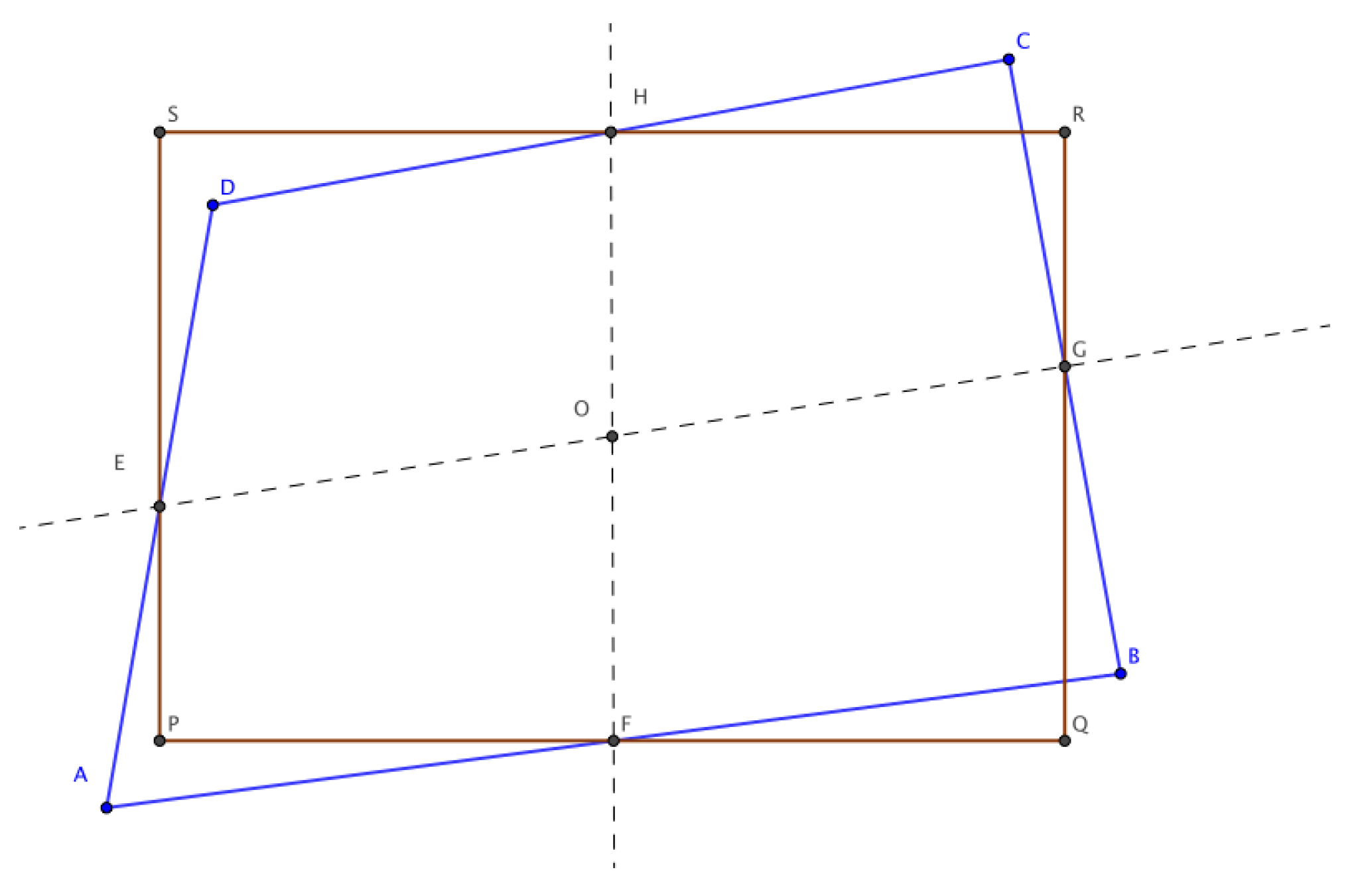
We propose the use of the rectangle of minimum area to define a distortion measure of the quadrilateral in the sense that it measures how close or far a quadrilateral Q is from being a rectangle, Figure 2.

Example 1.

For the quadrilateral A(−6.84, 7.5), B(−10, −4), C(11.81, −1.38) and D(9.27, 11.94), the rectangle of minimum area is $A^{\prime }BC{D}^{\prime }$ with an aspect ratio of 1.62. See Figure 2.

On one hand, the cell area $a_c$, is less than the rectangle area; that is, $a_c\le a_R$, and it is easy to see that

$$\frac{2a_c-a_R}{a_R}\le 1;$$

see Lassak [12] for the proof. The quotient thus defined reaches its maximum value of 1 on rectangles. Therefore, we propose the value

$${\mu }_{r1}\left(Q\right)=\frac{2a_c-a_R}{a_R}$$

(10)

as a new quality measure to characterize rectangles.

One must note that ${\mu }_{r1}\left(Q\right)$ is a good quality measure according to Field-Oddy, and ${\mu }_{r1}\left(Q\right)=0$ if Q is a triangle.

Another good quality measure in this sense is

$${\mu }_{r2}\left(Q\right)=\frac{2a_{-}}{a_R},$$

(11)

where

$$a_{-}=min\left\{a_1,a_2,a_3,a_4\right\}$$

(12)

and $a_i$ are the area of the four triangles defined by taking the four vertices of a quadrilateral into groups of three.

3.2. New Aspect Ratio

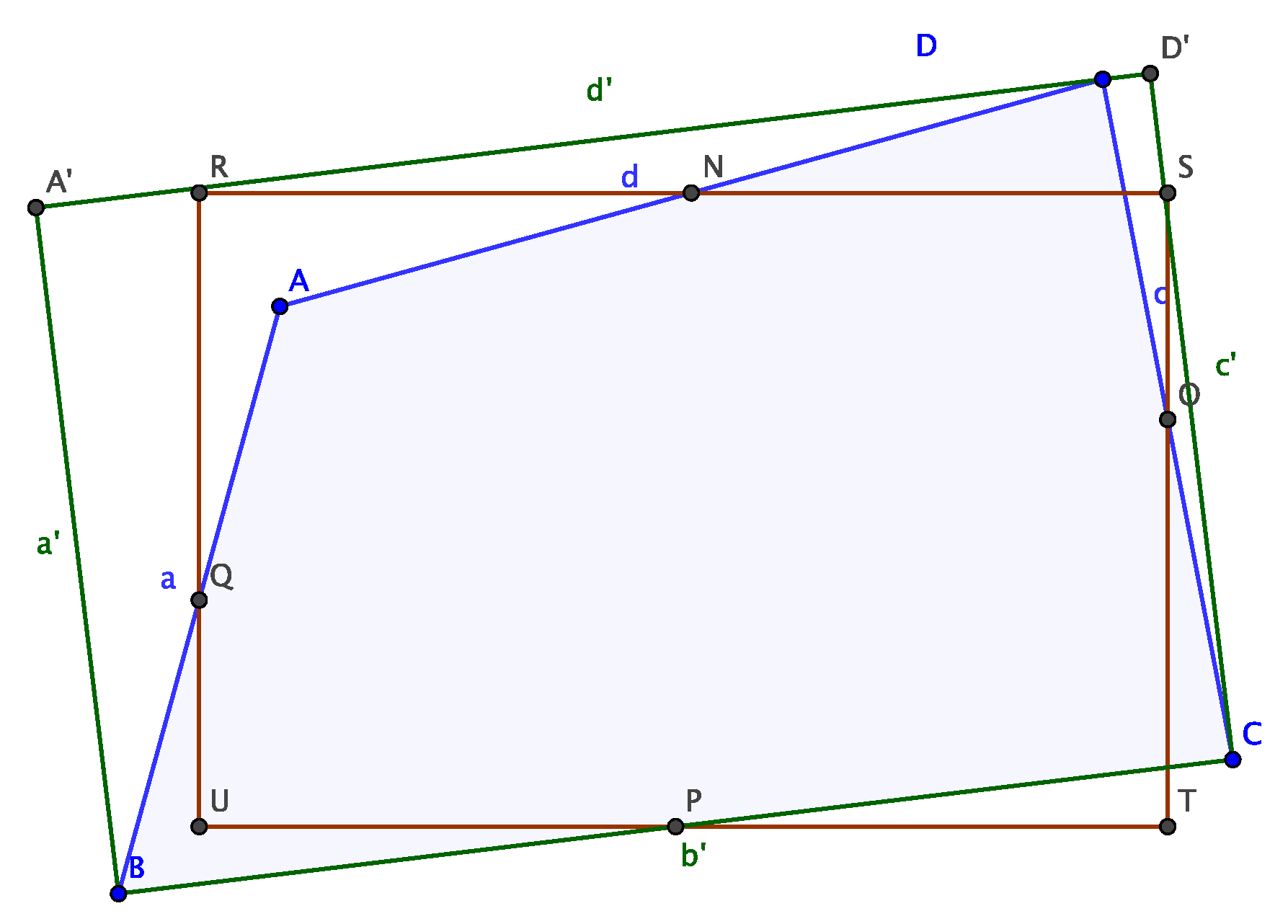
Using the rectangle of minimum area for Q, we propose the use of the ratio of the largest to the smallest side as the aspect ratio. This measure is invariant under rigid and scaling transformations. This measure is better than Robinson’s aspect ratio. It is easy to construct an example for which the Robinson aspect ratio is 1 but the quadrilateral is distorted following the next example.

Example 2.

For the quadrilateral A(3.53, 10.21), B(−10, −4), C(11.81, −1.38) and D(9.27, 11.94), Robinson’s aspect ratio is 1.00 but using the rectangle of minimum area $NBCD$, the aspect ratio is 1.62. See Figure 3.

As we have discussed, some measures to characterize rectangles are based on the inner angles. Another way to achieve this is to ask Q to be a parallelogram and one of its inner angles to be a right one. As it is, we use a measure that imposes a particular condition on a rectangle instead of one on the form of Q.

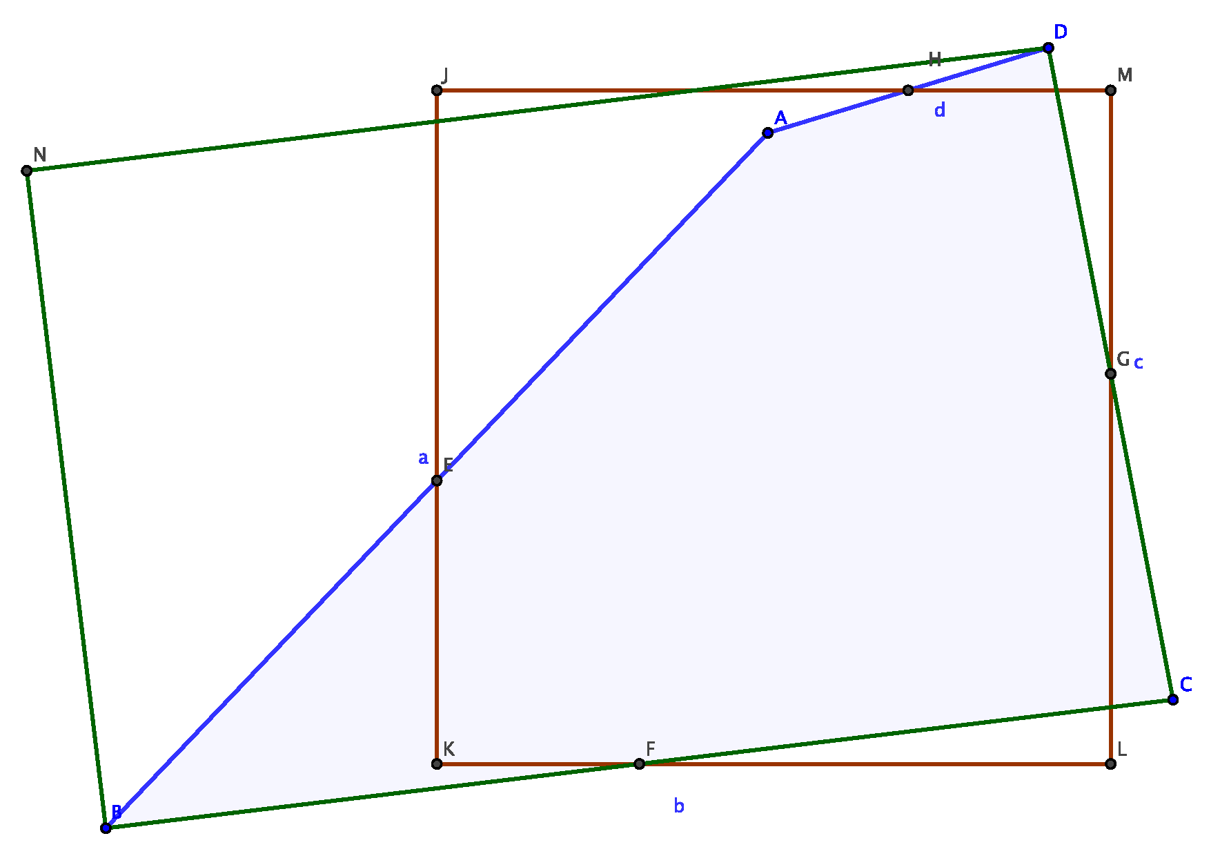
Our interest is to characterize the rectangles geometrically. A well-known result in the literature is as follows:

Theorem 1.

Let Q be a quadrilateral of vertices $A,B,C$ and D whose sides are $a,b,c$ and d. The quadrilateral Q is a rectangle if and only if the area of the quadrilateral is written as

$$a_R=\frac{1}{2}\sqrt{(a^2+c^2)(b^2+d^2)}.$$

(13)

The proof of this result can be found in Josefsson [13]. The interesting fact about this theorem is that it provides of an analytical expression of the area of a hypothetical rectangle formed by the sum of the squares of the opposite sides of Q and compares the square of the area of Q to identify how far it is from being a rectangle.

On the other hand, following the proof of the theorem, it is easy to see that the area $a_c$ of any convex quadrilateral satisfies

$$2a_c\le \sqrt{(a^2+c^2)(b^2+d^2)}.$$

(14)

Using this idea, we propose the measure

$${\mu }_R\left(Q\right)=\frac{2a_{-}}{\sqrt{(a^2+c^2)(b^2+d^2)}}$$

(15)

where $a_{-}$ is defined in Equation (12).

The measure ${\mu }_R\left(Q\right)$ is a good quality measure in the Field-Oddy sense, since it is continuous, bounded and capable of indentifying degenerate quadrilaterals (to triangles), as well as to identify if a quadrilateral is non-convex. This measure reaches its optimal value of 1 for rectangles.

An acceptability interval to consider that the quadrilateral is a rectangle under this measure is $[0.95,1]$.

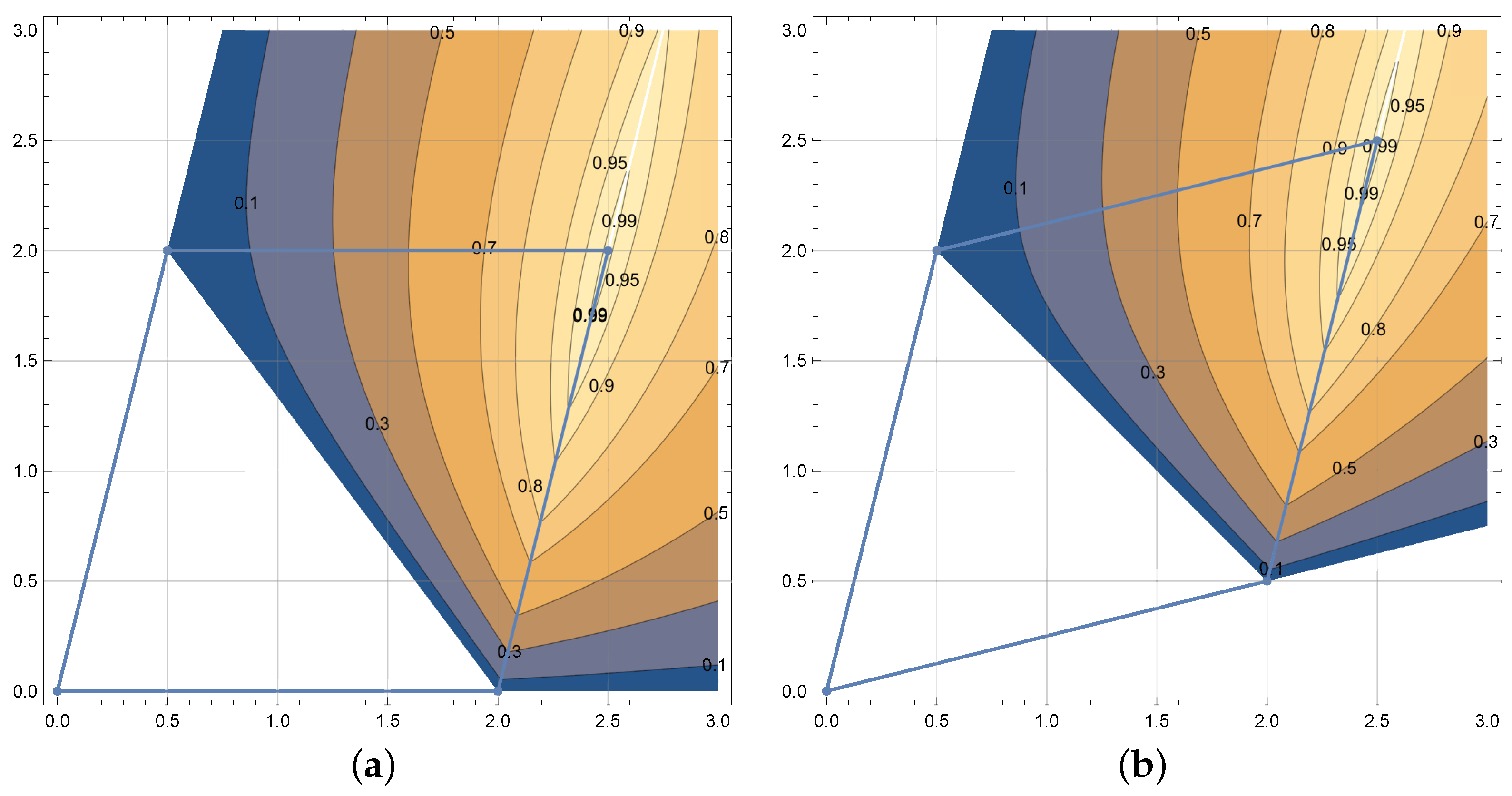
3.3. Quality Measure of Parallelograms

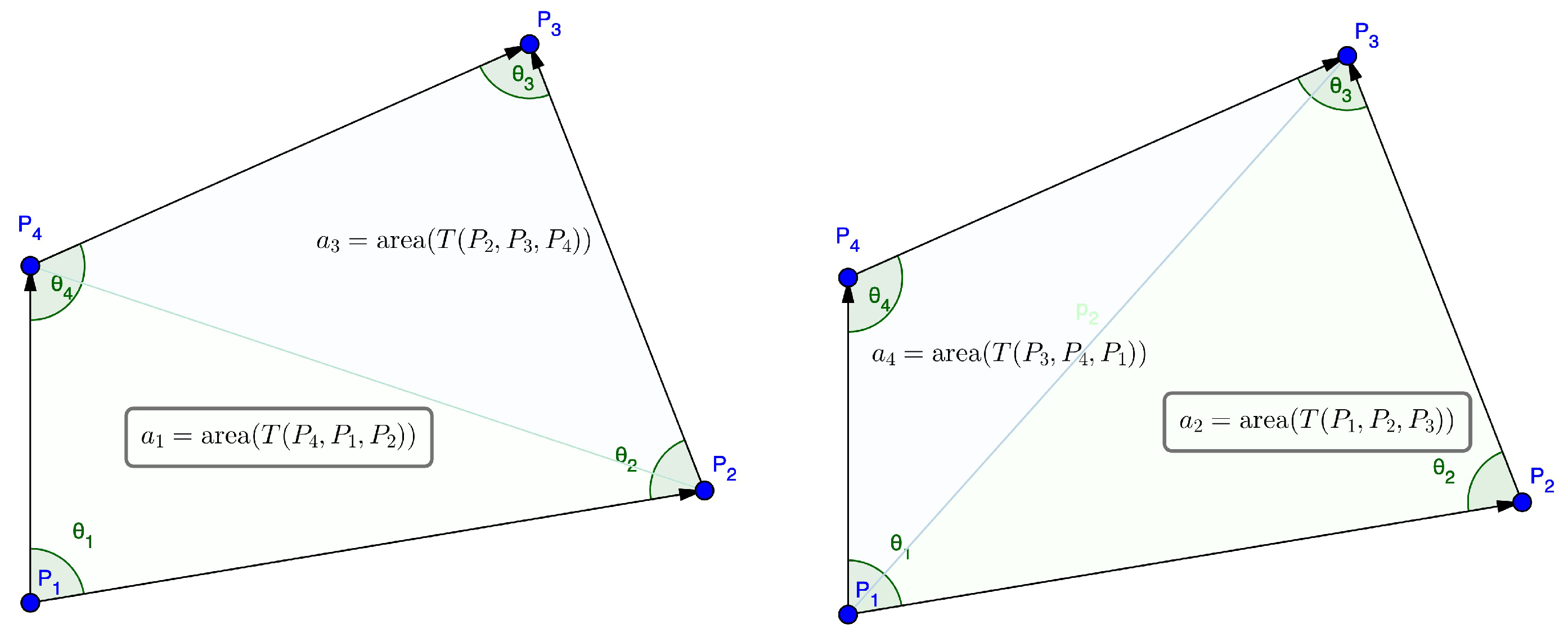
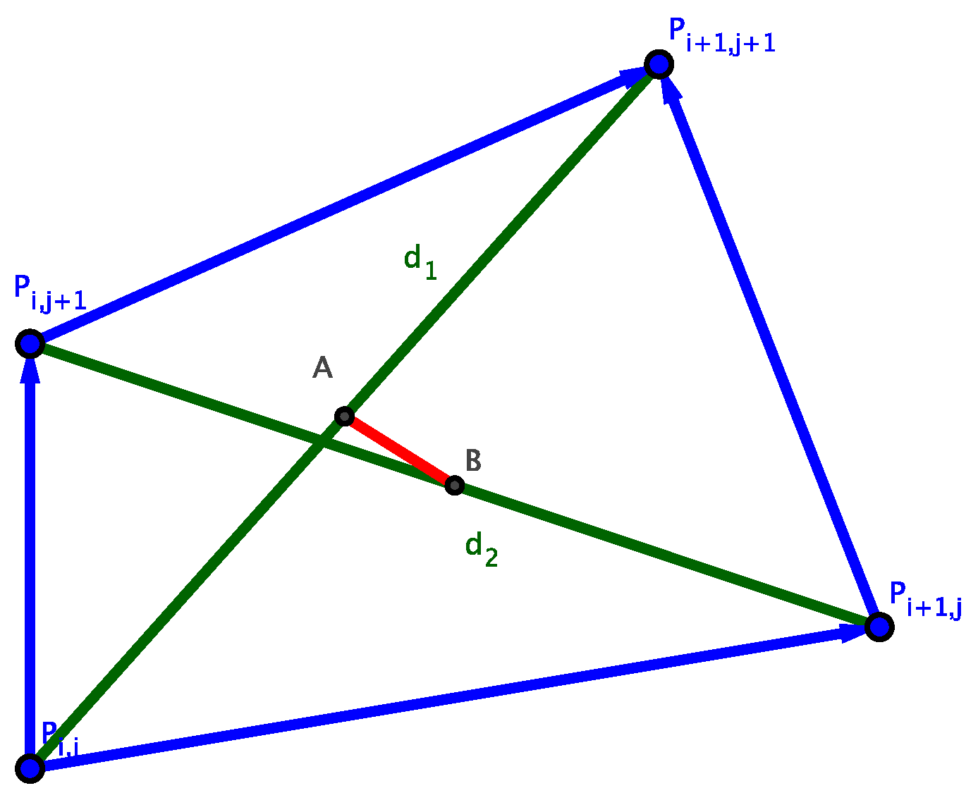
Let Q be an oriented quadrilateral of vertices $P_1{P}_2{P}_3{P}_4$. The latter defines four oriented triangles $T_1=T(P_4,P_1,P_2)$, $T_2=T(P_1,P_2,P_3)$, $T_3=T(P_2,P_3,P_4)$ and $T_4=T(P_3,P_4,P_1)$, see the Figure 4.

Let $a_i$ be the area of the four oriented triangle and $a_c$ be the area of grid cell Q, we have

$$g_1=\frac{a_1}{a_c},g_2=\frac{a_2}{a_c},g_3=\frac{a_3}{a_c},g_4=\frac{a_4}{a_c}$$

(16)

It is easy to see that a quadrilateral is a parallelogram if and only if

$$g_1{g}_2=g_3{g}_4=\frac{1}{4},$$

(17)

The proof is based on follow: on one side

$$g_1+g_3=g_2+g_4=1.$$

(18)

On the other hand

$$g_1=g_2$$

(19)

if and only if corresponding sides are parallel. But if we impose that g₁ and g₂ are equal $1/2$, $g_3=g_4$ so that the other sides are parallel, see [4]. A quality measure to characterize parallelograms is

$${\mu }_{p1}\left(Q\right)=4min\{g_1{g}_2,g_3{g}_4\}.$$

(20)

This measure is invariant under rigid and scaling transformations.

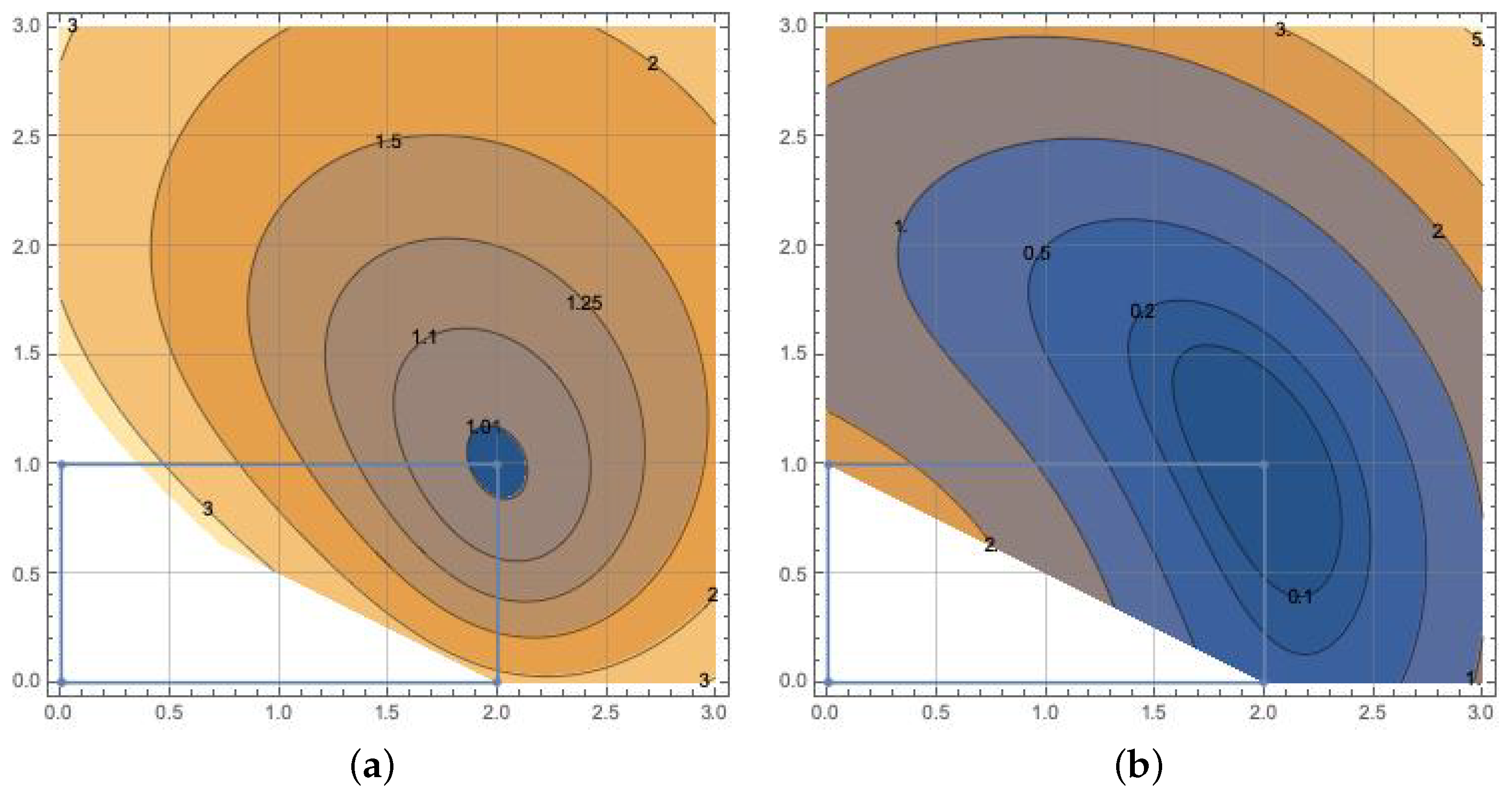
In the Figure 5 it is shown differents level curves for ${\mu }_{p1}\left(Q\right)$.

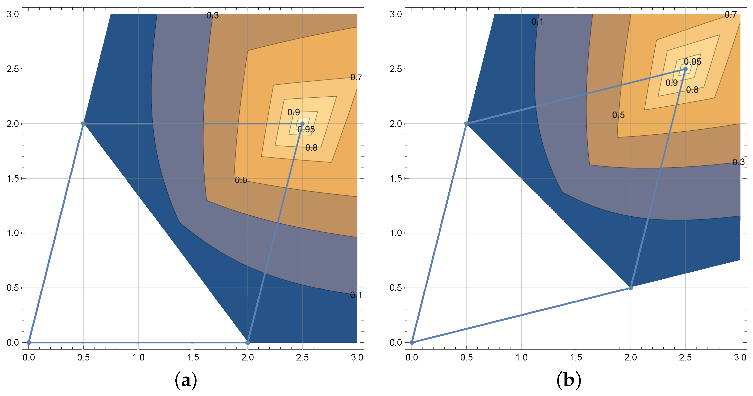
Now, we reorder these quantities in such a way that

$$g_1\le g_2\le g_3\le g_4,$$

(21)

and use

$${\mu }_{p2}\left(Q\right)=\frac{g_1{g}_2}{g_3{g}_4},$$

(22)

as a quality measure. Again, the maximum value is 1 and it is obtained for parallelograms. This is a quality measure because it is continuous, bounded and identifies degenerate and even non-convex quadrilaterals, see [4].

In the Figure 6 it is shown different level curves for ${\mu }_{p2}\left(Q\right)$.

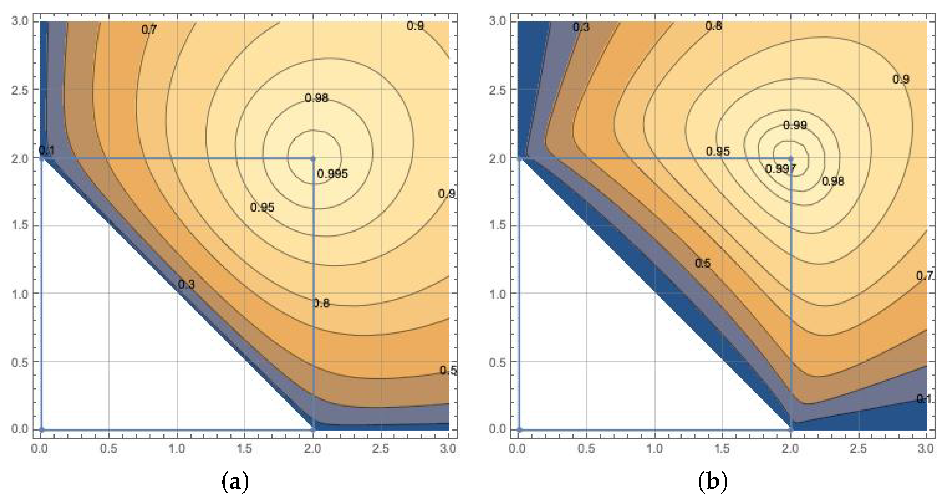
3.4. Quality Measure of Squares

An ideal mesh is one in which its cells are close to being squares. If $\mu \left(T\right)$ is a good quality measure for triangles, the harmonic mean of the four triangles $T_i$ is

$${\mu }_s\left(Q\right)=\sigma \frac{4}{{\sum }_{i=1}^4\frac{1}{\mu \left(T_i\right)}},$$

(23)

If rewriting ${\mu }_s\left(Q\right)$ in the form

$${\mu }_s\left(Q\right)=\frac{4\sigma \mu \left(T_1\right)\mu \left(T_2\right)\mu \left(T_3\right)\mu \left(T_4\right)}{\mu \left(T_2\right)\mu \left(T_3\right)\mu \left(T_4\right)+\mu \left(T_1\right)\mu \left(T_3\right)\mu \left(T_4\right)+\mu \left(T_1\right)\mu \left(T_2\right)\mu \left(T_4\right)+\mu \left(T_1\right)\mu \left(T_2\right)\mu \left(T_3\right)},$$

(24)

we obtain a good quality measure for quadrilaterals, because it is continuous, bounded, invariant under the rigid and scaling transformations and identifies degenerate and even non-convex quadrilaterals, since it inherits those properties from $\mu \left(T\right)$. Here, $\sigma$ is a normalization parameter.

To characterize squares, we require a property $\mu \left(T\right)$ as seen from:

Theorem 2.

If $\mu \left(T\right)$ is a good quality measure for triangles according to Field-Oddy, in which for isosceles right triangle the highest energy among all right triangles is achieved, ${\mu }_s\left(Q\right)$ defined in (24) is a quality measure in the Field-Oddy sense and characterizes squares at their maximum value.

Proof. 

The proof is very simple; it is based on the fact that the four triangles must be congruent to have the same energy. From this it follows that the triangles must be right triangle or they do not form a quadrilateral. Now, if the lowest energy contained for right triangle only occurs when they are isosceles right triangle then ${\mu }_s\left(Q\right)$ defined in (24) only detects squares at its maximum value.

Some measures $\mu \left(T\right)$ for triangles with those properties are

$${\mu }_1\left(T\right)=4\sqrt{3}\frac{A}{l_1^2+l_2^2+l_3^2},{\mu }_2\left(T\right)=2\frac{r}{R},{\mu }_3\left(T\right)=\frac{4\sqrt{3}}{9}\frac{A}{R^2},{\mu }_4\left(T\right)=\frac{4}{\sqrt{3}}\frac{A}{l_{max}^2}$$

where ${\mu }_1\left(T\right)$ was proposed by Joe, [14], ${\mu }_2\left(T\right)$ is the radius ratio measure, ${\mu }_3\left(T\right)$ is described by Shewchuk and ${\mu }_4\left(T\right)$ is Cavendish’s measure, see [15].

Using the quadrilateral Q with 3 fixed vertices $(0,0),(2,0)$ and $(0,2)$, $\mu \left(Q\right)$ is a function of $(x,y)$. In the Figure 7 it is shown the level curves for ${\mu }_s\left(Q\right)$ using ${\mu }_1\left(T\right)$ and ${\mu }_2\left(T\right)$. □

4. Some Global Quality Metrics

In many applications, it is necessary to identify the utility of a mesh through the assessment of the quality of all the mesh elements.

The assessment of the quality of a mesh can be achieved through

(1)

A visual or exploratory or inspection;

(2)

Qualitative evaluation or shape parameters;

(3)

Statistical analysis.

A first visual evaluation can involve analyzing the distribution in a histogram of values of a chosen good-quality measure $\mu \left(Q\right)$ or metric $\delta \left(Q\right)$. A second visual assessment can be performed by looking at a color map on a quality-dependent color scale. In this section, we will attempt to describe some methods or techniques with which to carry out a global qualitative assessment of the mesh by assigning a value to the mesh.

Allievi and Casal [16] proposed two measures for qualitative evaluation of orthogonality of the mesh. The first criteria is the maximum deviation of orthogonality given by

$$\mathrm{M}\mathrm{D}\mathrm{O}=\underset{i,j}{max}\left\{\right|{90}^{\circ }-{\theta }_{i,j}\left|\right\}$$

(25)

and the second is the mean deviation of orthogonality given by

$$\mathrm{A}\mathrm{D}\mathrm{O}=\frac{1}{(n-1)(m-1)}\sum _{i=2}^{m-1}\sum _{j=2}^{n-1}|{90}^{\circ }-{\theta }_{i,j}|,$$

(26)

where ${\theta }_{i,j}$ are the internal angles of the mesh.

Now, let $\mu \left(Q\right)$ be a measure of quality. Other global criteria used frecuently is the average quality of a mesh G, or the mean quality, defined as

$$MQ=\overline{\mu }\left(G\right)=\frac{1}{N}\sum _{i=1}^N\mu \left(Q_i\right),$$

(27)

where N is the number of elements in G. Another global measure well known is the standard deviation or the mean square error:

$$MSE={\sigma }^2=\sqrt{\frac{1}{N}{\displaystyle \sum _{i=1}^N}{(\mu \left(Q_i\right)-\overline{\mu }\left(G\right))}^2},$$

(28)

which is a value that represents the averages of all the individual differences of the observations with respect to a common reference point, which is the arithmetic mean.

As it is well known, a greater value of $MSE$ corresponds to a greater dispersion of the values, in this case $\mu \left(Q\right)$ with respect to its mean $MQ$. For this reason, researchers are using the geometric mean as a measure of global quality of the mesh for a measure $\mu \left(Q\right)$ given by

$$SP=\beta =\sqrt[N]{{\displaystyle \prod _{i=1}^N}\mu \left(Q_i\right)}.$$

(29)

This quantity is well known in the literature as the mesh shape parameter or simply shape parameter, see [2].

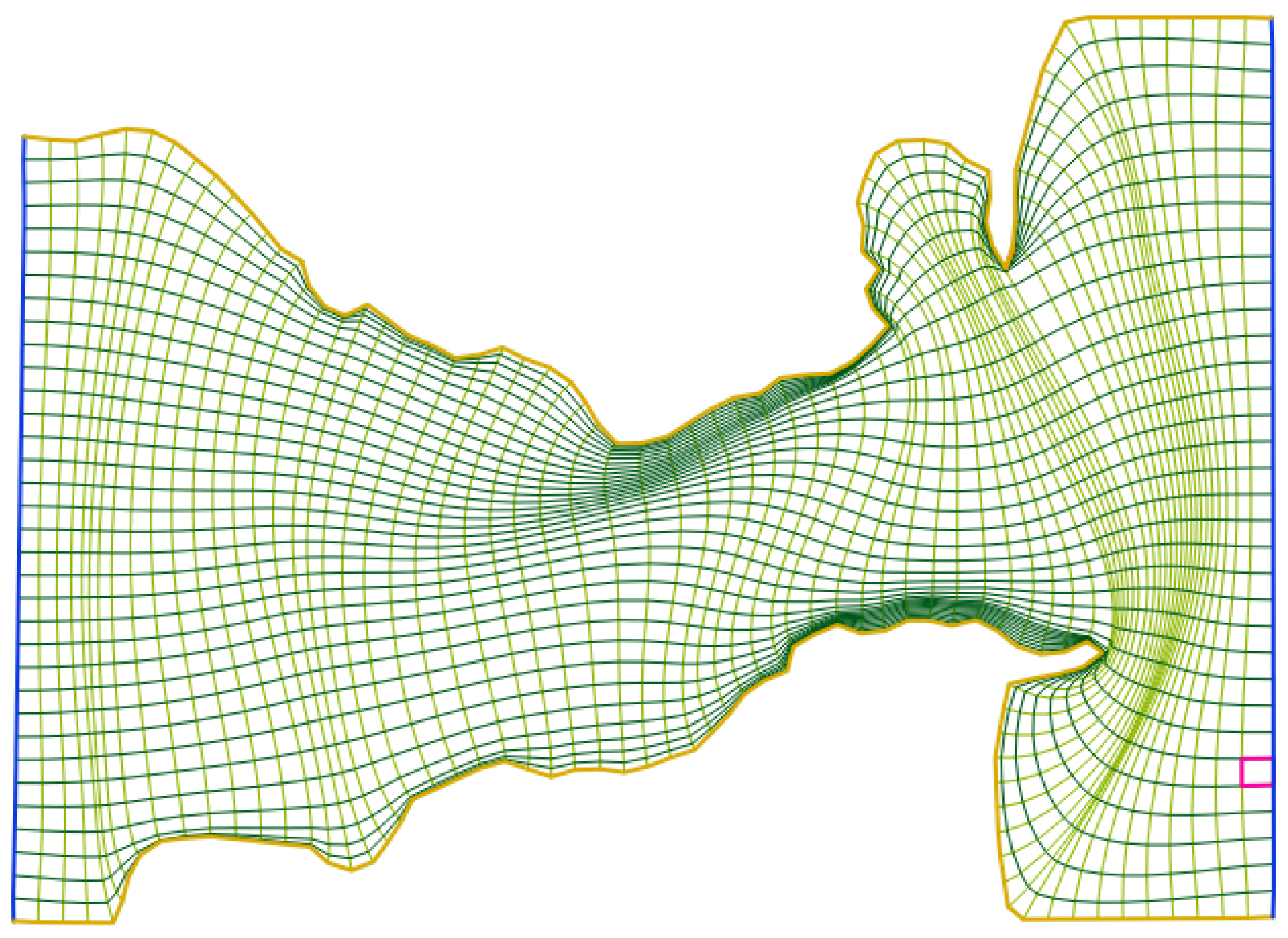
The natural approach to evaluate the quality of an mesh from that of its elements consists of considering the best and worst element qualities, the arithmetic mean, the mean square error and the shape parameter. For the mesh of the Figure 8 with ADO = 13.21, MDO = 76.17, the corresponding results for differents quality measures are given in

Table 1. Summary of quadrangle quality measures for the mesh in Figure 8.

Shape	Name $\mathit{\mu }\left(\mathit{Q}\right)$	Min	Max	MQ	MSE	SP
Parallelogram	AreaI	0.0381	0.9998	0.9169	0.1081	0.9068
	AreaII	0.0117	0.9973	0.8615	0.1510	0.8284
Rectangle	Lo1989	0.0160	0.9941	0.7597	0.1901	0.7241
	ScaledJacobian	0.2391	1.0000	0.9384	0.0975	0.9318
	ScaledJacobianM	0.0457	0.9965	0.8639	0.1361	0.8478
	MinRect2015	0.0555	0.9942	0.7929	0.1837	0.7607
	Rectangles2015	0.0719	0.9983	0.8999	0.1170	0.8890
Square	Lo1985	0.0339	0.9897	0.4792	0.2362	0.4162
	Hua1995	0.0830	0.9996	0.5302	0.2573	0.4621
	Knupp2000	0.0365	0.9993	0.5113	0.2588	0.4402
	Pebay2002	0.0591	0.9814	0.6119	0.2208	0.5670
	Hmean2017E	0.0797	0.9996	0.5292	0.2578	0.4607
	Hmean2017R	0.0788	0.9996	0.5292	0.2578	0.4606
	Hmean2017r	0.0297	0.9996	0.5351	0.2485	0.4713

.

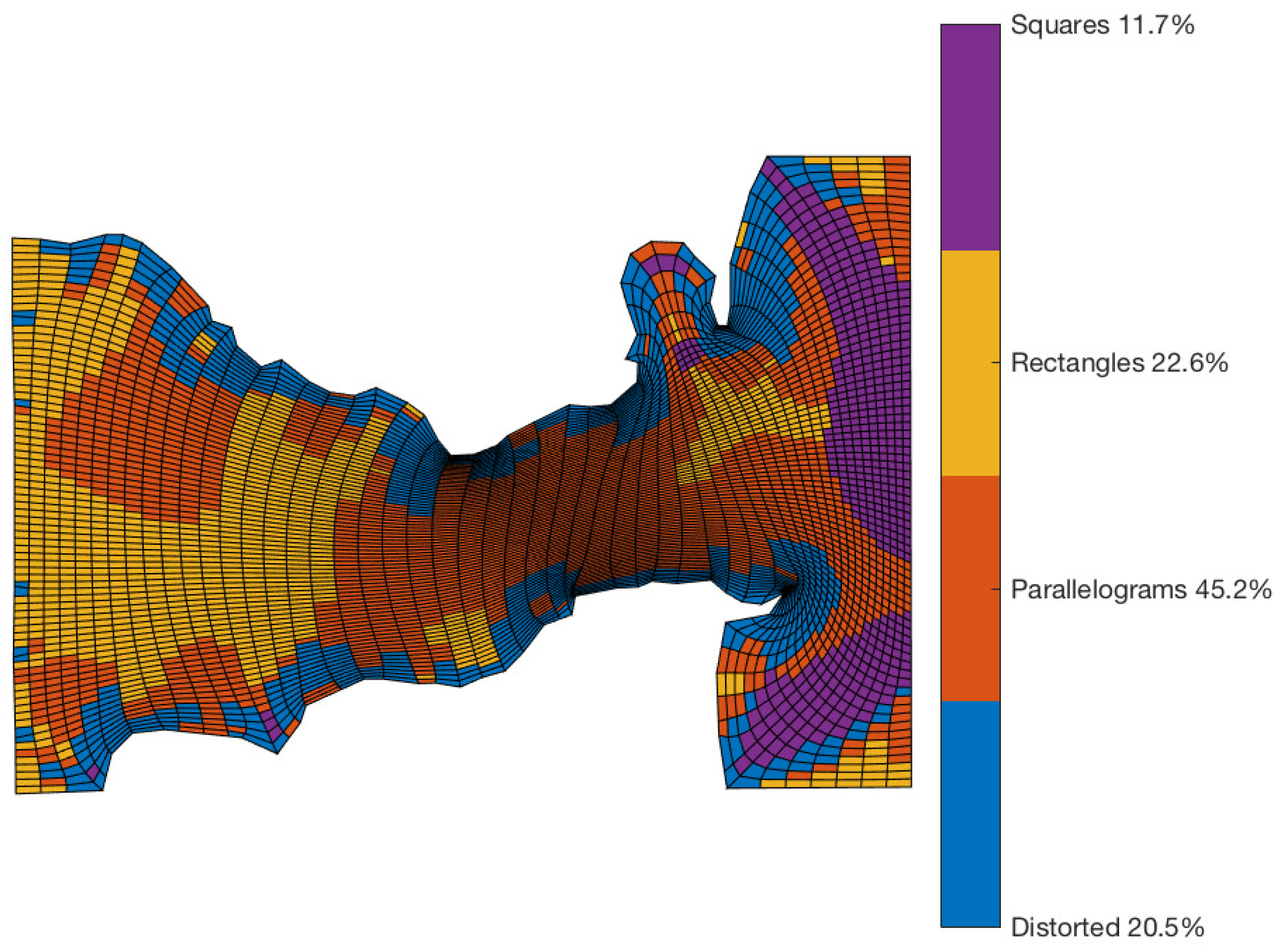
We believe that a statistical approach should be used to qualify and quantify the geometric quality of a mesh. The shape parameter for squares or rectangles can be combined with a statistical analysis of all the elements of the mesh in the following order:

(1)

How many elements are squares?

(2)

How many elements are rectangles with aspect ratio less than 4?

(3)

How many elements are parallelograms with aspect ratio less than 4?

We will say that the remainer cells are distorted. This can be performed as follows: consider three measures of quality ${\mu }_s\left(Q\right)$, ${\mu }_r\left(Q\right)$ and ${\mu }_p\left(Q\right)$ for squares, rectangles and parallelograms, and exclude rectangles from squares and parallelograms from rectangles. Let us exclude, respectively, large-aspect-ratio rectangles and large skew elements. Now let us represent those elements in a colormap, see Figure 8.

This technique can be very useful for meshes over irregular regions such as lakes or reservoirs.

In this paper the quality measure for curved elements are not discussed, but a good reference for curvilinear finite elements is [17].

5. Grid Quality Improvement

On Distortion of the Mesh

In general, if $\mu \left(Q\right)$ is a good quality measure for quadrilaterals, a way of measuring the distortion of a quadrilateral Q with respect to $\mu \left(Q\right)$ is using

$$f\left(Q\right)=\frac{1}{\mu \left(Q\right)},$$

(30)

because if $f\left(Q\right)$ is much greater than 1, the cell will be far from the value for which $\mu \left(Q\right)$ characterizes the geometric shape of the cell Q (square, rectangle, parallelogram, etc.) and we can say that Q is a distorted quadrilateral with respect to that measure. Usually, the maximum value of a quality measure corresponds to the minimum value of the energy density over the grid, see Ivanenko [18].

Under this idea, the distortion of the mesh G can be measured as the average of the distortions of all the cells

$$F\left(G\right)=\frac{1}{Ne}\sum _{k=1}^{Ne}\frac{1}{\mu \left(Q_k\right)},$$

(31)

where $Ne$ its the number of the cells. Using this concept, we have the following definition:

Definition 2.

A grid $\widehat{G}$ has better quality than the mesh $\overline{G}$ if

$$F\left(\widehat{G}\right)<F\left(\overline{G}\right),$$

(32)

where $F\left(G\right)$ is a distorsion measure.

As an optimization problem, improving the quality of a G mesh can be considered as the problem

$$G^{*}=arg\underset{G}{min}F\left(G\right)=\frac{1}{Ne}\sum _{k=1}^{Ne}\frac{1}{\mu \left(Q_k\right)},$$

(33)

where the inner nodes of G are the unknowns. In this context, the discrete grid generation problem can be posed, in general, as a large scale optimization problem. The optimization problem is a large-scale one when the mesh dimensions $m\times n$ are very large. It is important to note that the initial mesh $G_0$ must be convex and remain so in each step of the optimization process. We use for this a Newton-like methods with bound constraints L-BFGS-B [19].

Usually, the quality measures for quadrilaterals are non-differentiable functions; in an optimization process, it is better to build a convex function with similar characteristics to the quality measure.

6. New Quality Discrete Functionals

From the proof of Theorem 1, it is easy to see that

$$2a_c\le \sqrt{(a^2+c^2)(b^2+d^2)},$$

(34)

for any convex quadrilateral, then

$$f_R\left(Q\right)=\frac{(a^2+c^2)(b^2+d^2)}{4a_c^2},$$

(35)

is a positive convex function whose critical points are rectangles. With this function, we can define a discrete functional $F_R\left(G\right)$ over all the grid cells

$$F_R\left(G\right)=\frac{1}{Ne}\sum _{k=1}^{Ne}{f}_R\left(Q_k\right).$$

(36)

In Figure 9, the shape of the surface of $F_R$ is sketched.

We propose to combine this functional with a convex area functional $S_w\left(G\right)$ defined in [3]. This functional has an infinite barrier at the boundary of the set of unfolded grids.

$$F\left(G\right)=(1-\sigma )S_w\left(G\right)+\sigma F_R\left(G\right),$$

(37)

where $\sigma >0$. In addition, the function

$$f_R\left(Q\right)=\frac{(a^2+c^2)(b^2+d^2)}{4a_c^2},$$

(38)

can be interpreted (by cells) as a normalization (with respect to the Jacobian) of Knupp’s area-orthogonality functional defined in [20]

$$f_{ao}\left(Q\right)=(a^2+c^2)(b^2+d^2).$$

(39)

As we have discussed, since the quality measures are usually non-differentiable functions, it is difficult to use them as objective functions; it is advisable to design the convex and differentiable functions $f\left(Q\right)$, whose optimal values also satisfy $\mu \left(Q\right)\approx 1$ for a specific quality measure $\mu \left(Q\right)$.

As it is known, a rectangle is a parallelogram, so its opposite sides are equal. The diagonals of a rectangle are equal and bisect each other. In Figure 10, we can see those elements.

With this idea, we propose to use a convex functional of the form

$$F_p\left(G\right)=\sum _{i,j}{\parallel \frac{{\mathbf{p}}_{i,j}+{\mathbf{p}}_{i+1,j+1}}{2}-\frac{{\mathbf{p}}_{i+1,j}+{\mathbf{p}}_{i,j+1}}{2}\parallel }^2,$$

(40)

over all elements of the grid G. Locally, this functional has a critical point in the cells formed by parallelograms, see Khattri [21].

Optimizing $F_p\left(G\right)$ is an attempt to produce parallelograms. Now, we define a discrete functional to obtain rectangles. For each cell of G let us measure the square of the difference of the square of diagonals

$$F_d\left(G\right)=\sum _{i,j}(\parallel {\mathbf{p}}_{i,j}-{\mathbf{p}}_{i+1,j+1}{\parallel }^2-\parallel {\mathbf{p}}_{i+1,j}-{\mathbf{p}}_{i,j+1}{{\parallel }^2)}^2;$$

(41)

combining both functionals, we obtain

$$F_r\left(G\right)=(1-\alpha )F_p\left(G\right)+\alpha F_d\left(G\right).$$

(42)

If where $\alpha \ge 0$ is chosen to allow that shape of the cells can be flexible. In the practice we use $\alpha =0.5$. $F_r\left(G\right)$ is a positive and convex functional, which has a critical point in a mesh formed by rectangles (including squares). This can always be achieved if we guarantee that in each optimization step the mesh is convex.

Therefore, we use $S_w\left(G\right)$ to guarantee and preserve the convexity of the mesh, and combine it with the latter functional in the form

$$F\left(G\right)=(1-\sigma )S_{\omega }\left(G\right)+\sigma F_r\left(G\right).$$

(43)

Thus, with a linear convex combination between $S_{\omega }\left(G\right)$ and $F_r\left(G\right)$, one can generate both convex grid and close to being rectangles.

7. Examples

For both functionals, we can obtain optimal grids whose cells have a very large aspect ratio, see Figure 11.

Now, for control of the aspect ratio, we propose to use an area (volume) distortion measure functional

$$F_A\left(G\right)=\sum _{q=1}^N\frac{1}{\alpha {\left({▵}_q\right)}^2}+\delta \alpha {\left({▵}_q\right)}^2,$$

(44)

over all the N signed areas of all the grid cell triangles. Here, $\delta >0$ is an adequate value, see [4]. This distortion measure has a barrier on the boundary of the set of grids consisting of convex quadrilateral cells and it is very similar to the one proposed by Garanzha [22], but now we have a better control of the global distribution of the area.

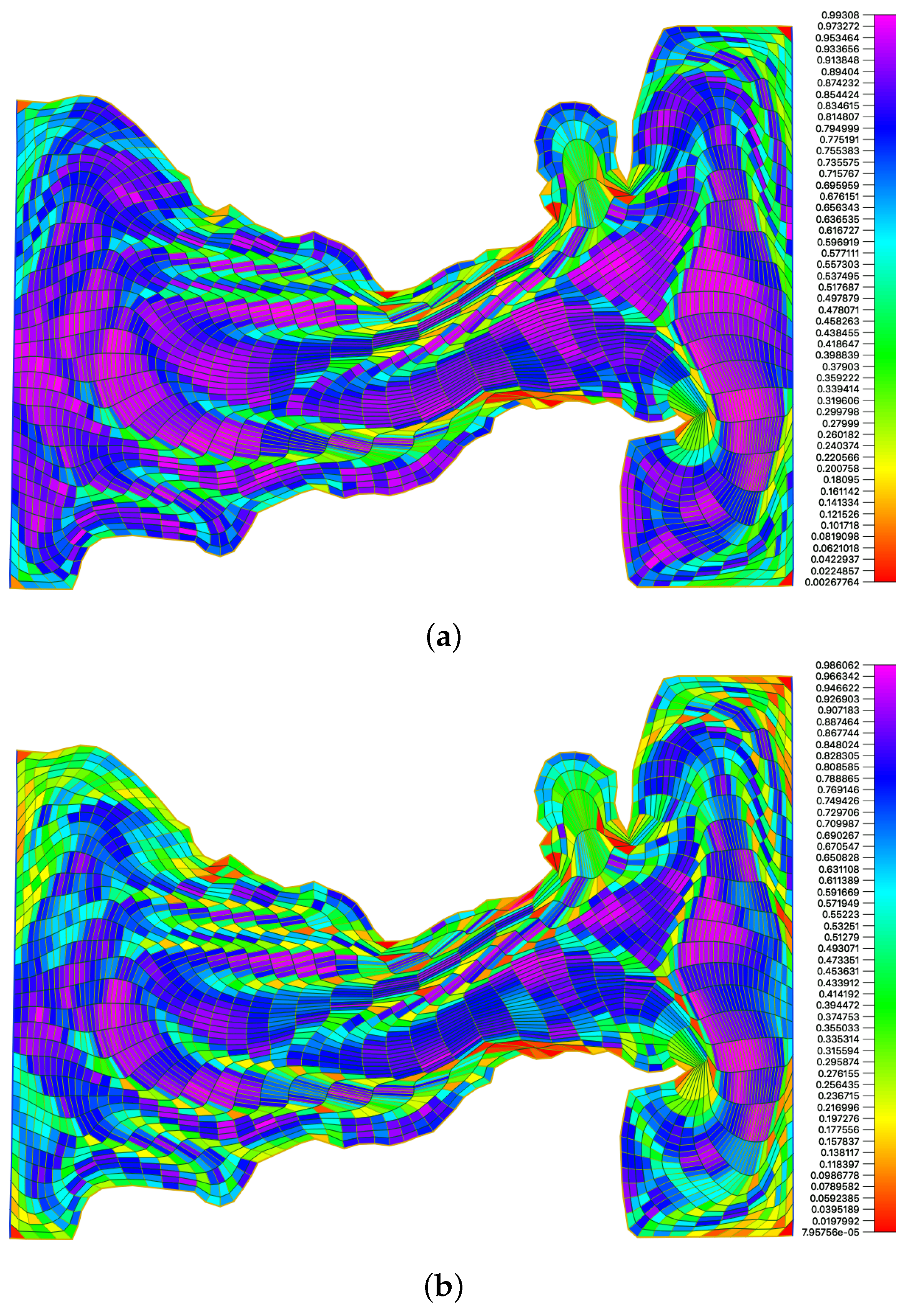
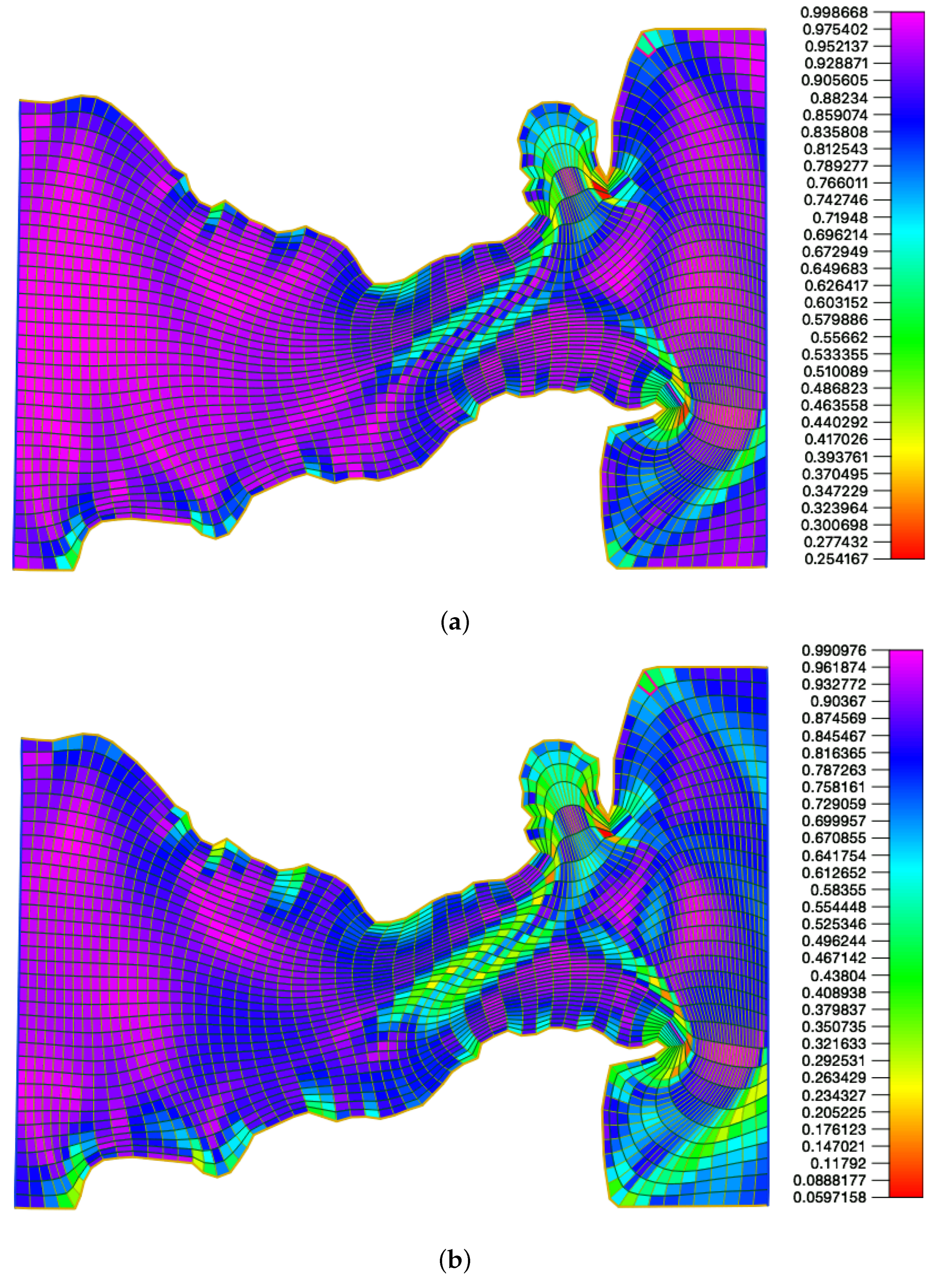
For the mesh optimized using the functional (37) with area control, we show in Figure 12 the color maps for two quality measures.

For the mesh optimized using the functional (43) with area control, we show in Figure 13 the color maps for two quality measures.

As it is well known, for irregular regions, the distorted cells accumulate near the border.

8. Conclusions

In conclusion, this paper presented an overview of classical quality measures and introduced new quality measures for quadrilaterals that help to improve meshes and the aspect ratio. We show that our aspect ratio is better than the one proposed by Robinson. We propose that a statistical approach should be used to qualify and quantify the geometric quality of a mesh. In addition, we have proposed new functionals for grid generation as alternatives for area-orthogonal grid generation. These functionals are based on the fact that the maximum value of a quality measure corresponds to the minimum value of the energy density over the grid.

Future work in this area could include extending some of these ideas to 3D, as well as exploring the potential of functionals for volume grid generation, which need to be further investigated.