Exploring the Potential of Mixed Fourier Series in Signal Processing Applications Using One-Dimensional Smooth Closed-Form Functions with Compact Support: A Comprehensive Tutorial

Abstract

This paper studies and analyzes the approximation of one-dimensional smooth closed-form functions with compact support using a mixed Fourier series (i.e., a combination of partial Fourier series and other forms of partial series). To explore the potential of this approach, we discuss and revise its application in signal processing, especially because it allows us to control the decreasing rate of Fourier coefficients and avoids the Gibbs phenomenon. Therefore, this method improves the signal processing performance in a wide range of scenarios, such as function approximation, interpolation, increased convergence with quasi-spectral accuracy using the time domain or the frequency domain, numerical integration, and solutions of inverse problems such as ordinary differential equations. Moreover, the paper provides comprehensive examples of one-dimensional problems to showcase the advantages of this approach.

1. Introduction

The Fourier series of a function with compact support, denoted by g:$[0,T]\to \mathbb{R}$, has been the cornerstone of several modern applications through harmonic analysis and Fourier synthesis. On the one hand, harmonic analysis allows the study of the original function or phenomenon through the superposition of simpler trigonometric functions. This analysis represents a wide branch of study in mathematics [1,2,3] and is used in many applications in physics [4,5,6], engineering [7,8,9], medicine [10,11,12], and music [13]. Fourier synthesis, on the other hand, uses a linear combination of basis functions to approximate the original function [14], which has many applications in boundary value problems [15,16,17], data interpolation [18,19,20,21], and compression [22].

The Fourier series has several advantages for representing a function with compact support (i.e., non-periodic function). First, it has been extensively studied, and many well-known analytical and numerical properties can be applied [1,2]. Second, unlike other series based on local information, such as the Taylor series or the Spline series, the Fourier series does not require the use of high-order derivatives, and their coefficients are calculated by well-conditioned algorithms. Finally, unlike other series based on non-trigonometric basis functions using an inner product, such as orthogonal polynomials, the Fourier series offers the advantage of reducing the computational cost of obtaining the coefficients by employing the FFT (fast Fourier transform). However, despite those advantages, it is well-known that its performance degrades when the equivalent periodic function (denoted by $\overline{g}$:$\mathbb{R}\to \mathbb{R}$) loses its smooth property. The first shortcoming is the presence of unacceptable oscillations (i.e., ringing artifacts) in the approximation, which are generally known as the Gibbs (or Gibbs–Wilbraham) phenomenon [23]. The second shortcoming is slow convergence because the magnitude of Fourier coefficients is $O({\left|k\right|}^{-1})$ [24] or $O({\left|k\right|}^{-2})$ [25], which makes it difficult to obtain a suitable representation using few coefficients for many purposes, such as data compression or fast solvers of inverse problems. To address these drawbacks, several techniques have been proposed over the last several years. They can be classified into averaging and filtering techniques [26,27,28,29,30,31,32,33,34,35,36,37,38,39,40,41,42,43,44,45,46,47,48,49,50,51,52,53,54,55,56], polynomial techniques [57,58,59,60,61,62,63,64,65,66,67,68,69], and discontinuity subtraction techniques [70,71,72,73,74,75,76,77,78,79,80,81,82,83,84,85,86].

The Windowing technique [26] is possibly the most important filtering technique for harmonic analysis, in which the function is artificially smoothed with a relevant distortion cost for small bandwidths. Averaging and filtering techniques are more diverse for synthesis applications. For instance, the Fejér’s arithmetic mean method removes the Gibbs oscillations [27,28,29]. Similarly, the Lanczos sigma approximation [30,31,32], Mollifiers [33,34,35,36,37,38], and other averaging methods [39,40] and filters [41,42,43,44] can reduce ringing artifacts, too. Moreover, they can be combined with special wavelets [45,46,47,48,49,50] with the same purpose. Furthermore, these techniques can be merged with Fourier extension methods, in which artificial and convenient information in an extended interval $t\in [-a,T+a]$ allows for a reduction in undesirable phenomena in $t\in [0,T]$ [51,52,53,54,55,56]. Despite their success, averaging and filtering techniques have several drawbacks due to the artificial modification and slow convergence of the Fourier coefficients.

The main polynomial methodology for synthesis application may be the spectral reprojection approach [57], in which Fourier coefficients are reprojected onto other basis functions conformed by polynomials. For instance, the Gegenbauer polynomials [58,59,60] and general polynomials using inverse methods [61,62] are successful in removing the Gibbs phenomenon. In the same direction, Chebyshev polynomials produce a strongly nonuniform distribution of points with good performance for interpolation [63,64]. However, the solution loses simplification by using non-equidistant data. Similarly, other related techniques can address these concerns, such as Padé approximations [65,66,67], convergence acceleration, and inverse methods [68,69]. Although polynomial techniques reduce or remove ringing artifacts from arbitrary Fourier coefficients, they have some drawbacks due to their complexities or ill-conditioned solutions.

Discontinuity subtraction techniques are employed to separate the discontinuities in the original function, yielding a more convenient Fourier representation. To the best of our knowledge, the concept of removing discontinuities using polynomials was first introduced by Russian works in the 1900s. For instance, A. N. Krylov proposed the method of Acad using a piecewise linear polynomial [70], ([71], p. 79) and A. S. Maliev proposed a strengthened convergence method using high-order piecewise polynomials using a Fourier extension method ([71], p. 86). Those approaches were generalized by C. Lanczos in ([72], p. 98), using quasi-Bernoulli polynomials, denoted by $B_m\left(t\right)$, in the same domain of the function. The Maliev–Lanczos approach has enormous potential because it avoids the Gibbs phenomenon and allows for generating Fourier coefficients with convergence $O({\left|k\right|}^{-M})$. Despite the fact that these works demonstrated that the Fourier series can achieve accelerated convergence for smooth functions, there was little scientific discussion for almost three decades about these methods [77,78]. The Lanczos approach emerged again in the 1990s in the works of K. S. Eckhoff [79,80,81], who proposed the reconstruction of piecewise smooth functions with M jumps by solving a linear system of M equations using quasi-Bernoulli polynomials and the spectral domain. Over the last two decades, several Armenian researchers have made significant contributions to the Lanczos approach. For instance, the works of A. Nersessian and A. Poghosyan addressed the main issue of some alternatives to the quasi-Bernoulli series in [67,87,88,89,90,91,92], such as the quasi-polynomial series, the Fourier–Pade series, the trigonometric interpolations series, and the quasi-polynomial Pade series. Similarly, A. Nersessian studied a framework based on a biorthogonal system and adaptive algorithms with a strong potential for accelerating the convergence of Fourier series due to an over-convergence phenomenon [93,94,95,96]. Furthermore, some simplifications and applications of Eckhoff algorithm have been studied by A. Poghosyan et al. in [83,84,85,86,97], such as its application to two-dimensional functions, the simplification of the minimization problem, and the study of trigonometric interpolations series. Finally, several researchers around the world, who are not fully discussed in this introduction due to space limitations, have also contributed to this technique [82,98,99,100,101]. For example, B. Adcock provided a comprehensive discussion and evaluation of several related techniques in [99], and D. Batenkov proposed a novel decimated Eckhoff’s algorithm in [101].

On the other hand, Fourier series have been widely used to solve differential problems, such as ODEs, PDEs, and eigenvalues [14,102,103]. In particular, we found that, unrelated to the previous state of the art, P. Roache proposed the method of “reduction to periodicity” in [104] for solving differential equations in fluid dynamics [105,106]. That method applies the discontinuity subtraction technique using simple polynomials in a normalized domain (i.e., $\varphi \left(t\right)={\sum }_{k=0}^M{a}_k·t^k,\forall t\in [0,1]$), where the coefficients are chosen to produce a smooth periodic residual error, and therefore, the solution increases the convergence and removes ringing artifacts using the Fourier approach.

The Maliev–Lanczos approach to approximating closed-form smooth functions has four disadvantages in applied problems. First, the method requires explicit knowledge of the function’s derivative at the edges of the interval. However, for continuous-time applications where the closed-form function is known, this requirement does not cause setbacks because derivative operators may be easily computed using the chain rule. These continuous-time applications include the solutions to direct and inverse problems using linear operators (i.e., $\mathcal{L}\{·\}:g\to h$ such that $\mathcal{L}\{\alpha ·g_1\left(t\right)+\beta ·g_2\left(t\right)\}=\alpha ·\mathcal{L}\left\{g_1\left(t\right)\right\}+\beta ·\mathcal{L}\left\{g_2\left(t\right)\right\}$). Second, Fourier coefficients of the original function must be determined because the method is supported by the Fourier framework. For common functions, these coefficients are not always known in closed form. Third, the evaluation of quasi-Bernoulli polynomials requires an iterative algorithm that increases addition and product operations and, therefore, increases computation time and sensitivity to rounding errors in the operations $\mathcal{L}\left\{B_m\left(t\right)\right\}$. Finally, it would seem that the approach using quasi-Bernoulli polynomials is the best framework for accelerated convergence because they are directly found from integration by parts using the integral definition of Fourier coefficients.

Despite the advances of the last decades, the Maliev–Lanczos approach is not widely used or recognized as one would expect in continuous-time problems involving closed-form smooth functions in applied mathematics, physics, and engineering. For example, this technique receives minimal attention as an alternative to the Taylor series for non-analytic smooth functions on a closed interval. Unfortunately, the Maliev–Lanczos approach is rarely mentioned in engineering textbooks, despite the fact that the Fourier series and Taylor series are fundamental tools for a wide range of problems and applications (e.g., Riemann integration, integral equations, and boundary or initial value problems). Perhaps this is due to the aforementioned shortcomings, as well as a lack of useful information and discussions, canonical examples, or practical applications.

The contributions of this publication are categorized as follows. The first category involves making scientific contributions to the Maliev–Lanczos approach. This includes advancements, improvements, and novel insights related to the approach, which are listed below:

• We prove that the Roache approach (i.e., using simple polynomials derived from the residual error framework) is spectrally equivalent to the Lanczos approach (i.e., using quasi-Bernoulli polynomials derived from an integration-by-parts framework) for any harmonic different from zero (i.e., $\forall k\in \mathbb{Z}-\left\{0\right\}$), where simple polynomial coefficients are determined by a low-cost backward algorithm. Although both approaches have the same complexity when using linear operators based on integrals or derivatives, simple polynomials are easier to manipulate using these operators, and they reduce rounding errors by lowering addition and multiplication operations.
• We propose a reprojection method that allows the transformation from Fourier series coefficients to mixed Fourier series coefficients. We introduce the term “mixed Fourier series” to designate the summation of series derived from a smooth periodic residual error, wherein one of the series is the Fourier series. This method allows for recovering convergence $O({\left|k\right|}^{-M})$ using standard Fourier coefficients obtained from any smooth function. The proposed method has the advantage of avoiding the temporal information of g:$[0,T]\to \mathbb{R}$. Therefore, it has the potential to be particularly useful for native spectral applications (e.g., solving differential equations with spectral methods).
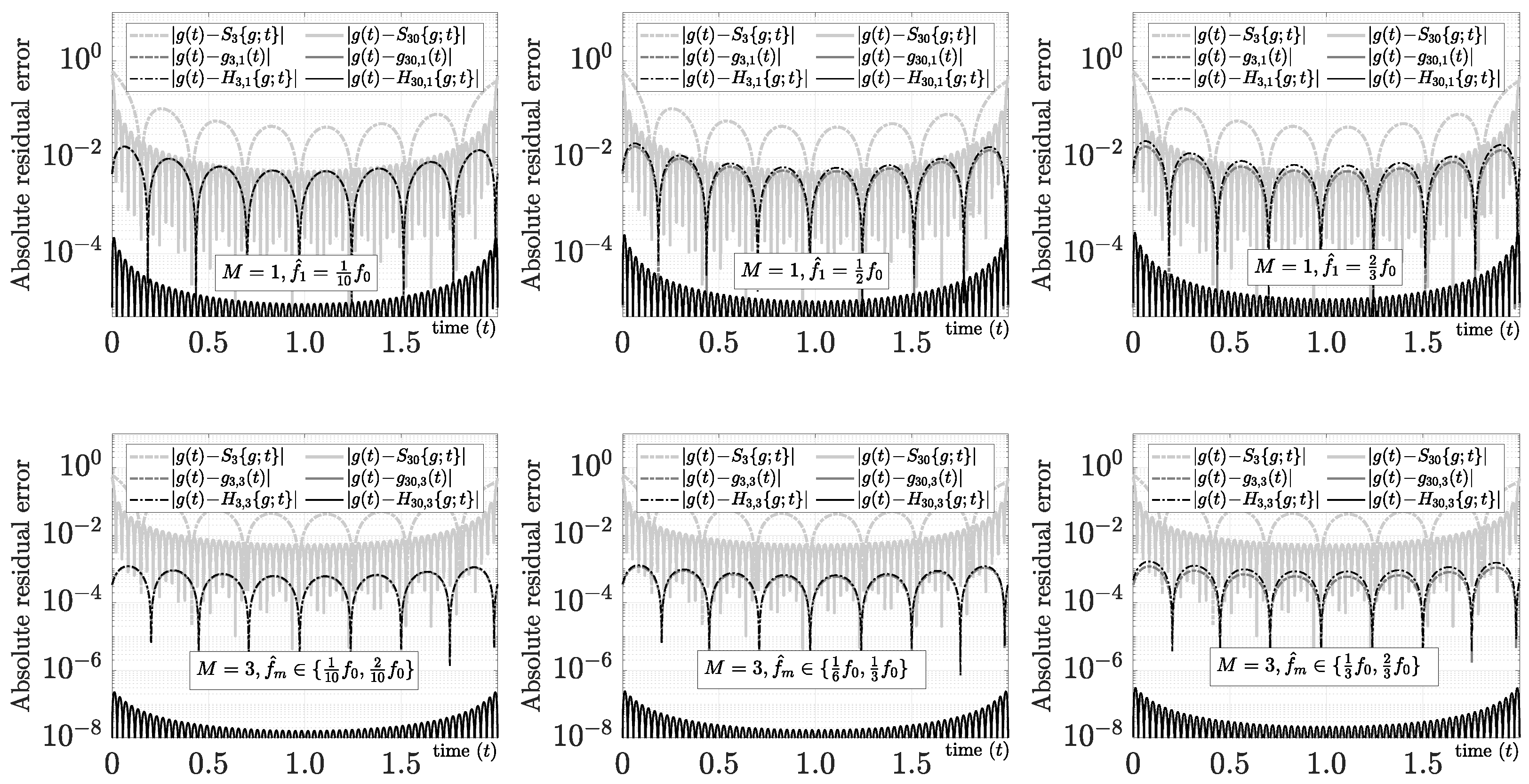
• By employing the Maliev–Lanczos approach and leveraging the residual error framework, we introduce and evaluate a novel sub-harmonic mixed Fourier series. This new series demonstrates enhanced performance and versatility in approximating wide-band or pass-band functions compared to the quasi-Bernoulli series. It is worth noting that the Maliev–Lanczos approach presents a set of continuity-based constraints that can be applied to any series complementing the Fourier series. Moreover, the conditions for achieving accelerated convergence can be readily obtained using the residual error framework.

The second category focuses on utilizing case studies as canonical examples to inspire and encourage non-specialists to apply the Maliev–Lanczos approach to real-life problems. The contributions pertaining to this category are listed below:

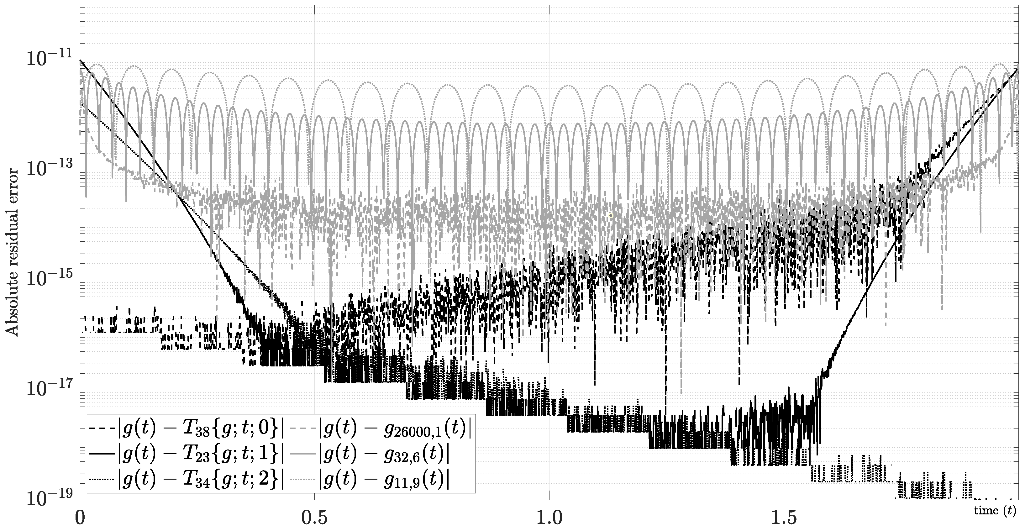
• We discuss several examples of common smooth functions whose approximations using polynomials and trigonometric series exhibit several well-known adverse phenomena, such as the Gibbs phenomenon, Runge’s phenomenon, spectral leakage, and non-convergence by a non-analytic point or a limited region of convergence (using the Taylor series), which are successfully represented by the mixed Fourier series. The results demonstrate the potential of the Maliev–Lanczos approach in the approximation of the usual smooth functions in applied problems, even outperforming, in several scenarios, the Taylor series, orthogonal polynomials, and Chebyshev polynomials using nonuniform sampling.
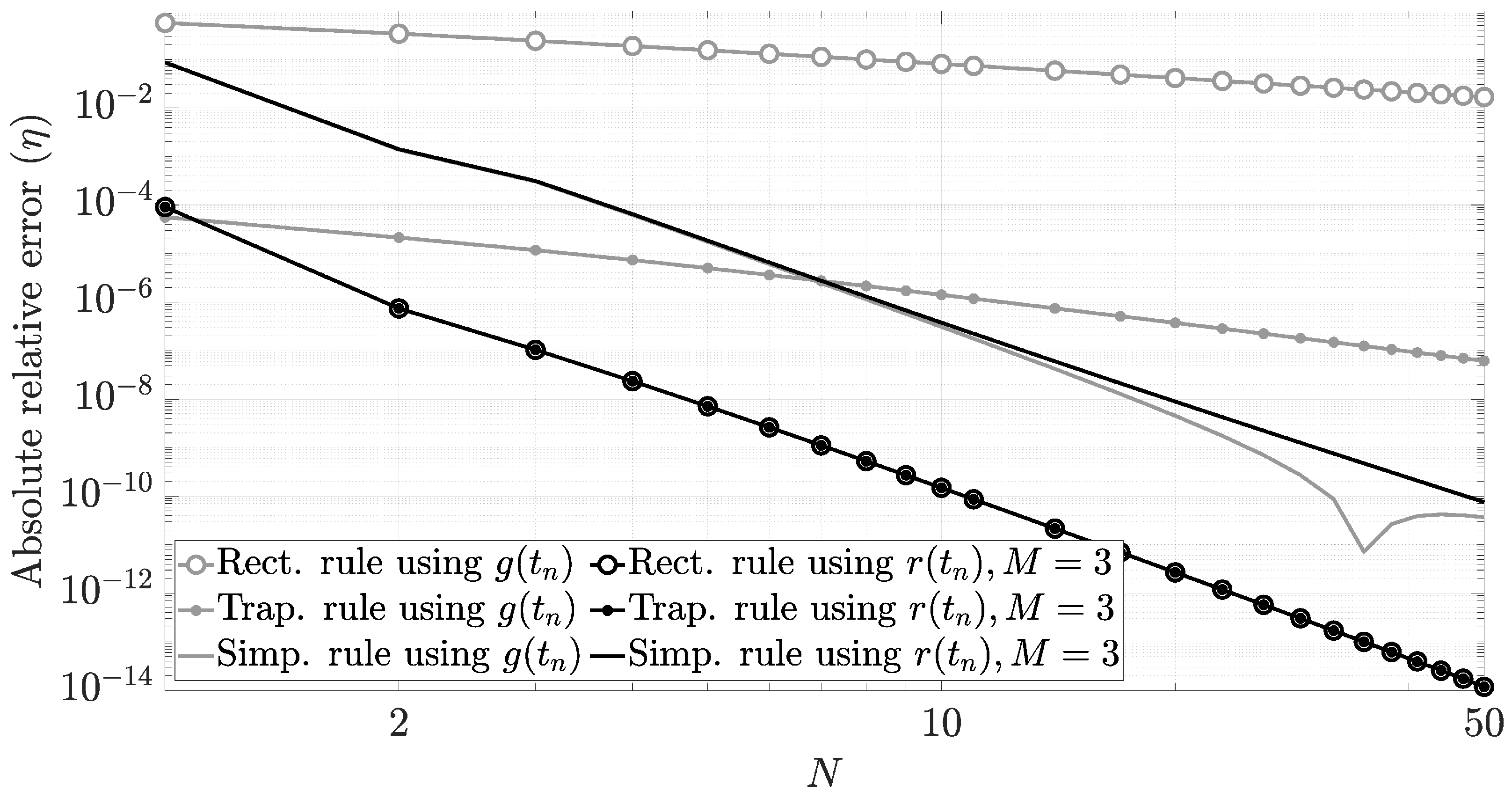
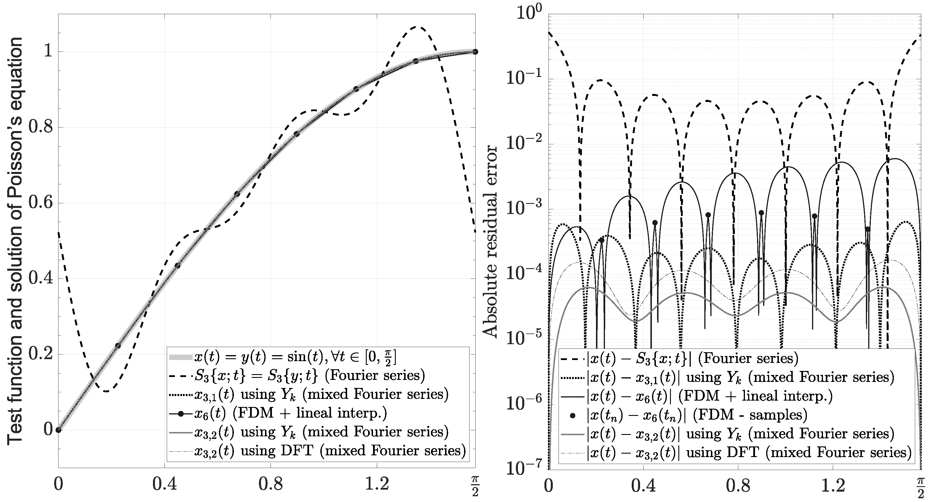
• We illustrate the application of the mixed Fourier series with linear operators. In particular, we solve a common direct problem in applied mathematics (Numerical Riemann Integration) and a common inverse problem in fluid dynamics (Poisson’s equation). In both examples, we show the benefit of employing simple polynomials, and we illustrate fast convergence without the Gibbs phenomenon.
• We evaluate the use of a mixed evaluation (i.e., a combination of closed-form derivatives and the DFT approach) to find the mixed Fourier series of functions without closed-form Fourier coefficients. In that case, we show that the DFT reflects the property $O({\left|k\right|}^{-M})$ for smooth functions, which allows accelerated discrete Fourier processing. Therefore, this approach has a huge potential for a wide range of practical situations.
• Finally, we show in detail the methodology used to define a new mixed Fourier series using the residual error framework. Additionally, the versatility of this new series is demonstrated through several examples.

The rest of this article is divided as follows. Section 2 develops the continuous-time theory, and Section 3 discusses several continuous-time examples and applications. Finally, the last sections present open challenges and future work (Section 4), followed by conclusions (Section 5).

2. Continuous-Time Theory

2.1. Fourier Series Fundamentals

Let g:$[0,T]\to \mathbb{R}$ be a function with compact support. Traditionally, the partial Fourier series of $g\left(t\right)$ is given by [3], p. 62

$$\begin{array}{cc}\hfill S_N\{g;t\}:& =\sum _{k=-N}^N{G}_k·e^{2\pi i·t·k{f}_0},\hfill \end{array}$$

(1)

where $f_0=\frac{1}{T}$, and the Fourier coefficients are

$$G_k:=\frac{1}{T}·\underset{0}{\overset{T}{\int }}g\left(t\right)·e^{-2\pi i·t·k{f}_0}dt,\forall k\in \mathbb{Z}.$$

(2)

This paper makes the assumption that $g\left(t\right)$ is a well-behaved (i.e., not pathological [107]) function such that ${lim}_{N\to \infty }{S}_N\{g;t\}\to g\left(t\right),\forall t\in [0,T]$ using a well-defined concept of convergence, such as point-wise, uniform, or based on the 2-norm (i.e., ${∥·∥}_2$) [1,2]. Moreover, the periodic equivalent function (denoted by $\overline{g}:\mathbb{R}\to \mathbb{R}$) is defined from the partial Fourier series by

$$\overline{g}\left(t\right):=\underset{N\to \infty }{lim}{S}_N\{g;t\},\forall t\in \mathbb{R}.$$

(3)

Definition 1. 

Let ${\mathcal{C}}^0[0,T]$ be the set of continuous functions on $[0,T]$. Let ${\mathcal{C}}^K[0,T]$ be the set of continuous functions with K-times continuously differential properties on $[0,T]$, where we use only the right-hand derivative definition at $t=0$ and the left-hand derivative definition at $t=T$.

Even though $g\left(t\right)$ has a smooth property, defined by $g\in {\mathcal{C}}^K[0,T]$, the Fourier series could be inefficient for analysis or synthesis applications because the periodic equivalent function could have discontinuities caused by the edges of the interval (e.g., $g\left(0^{+}\right)\ne g\left(T^{-}\right)\Rightarrow \overline{g}\left(m{T}^{+}\right)\ne \overline{g}\left(m{T}^{-}\right),\forall m\in \mathbb{Z})$. As a result, the periodic equivalent function is usually inconvenient for a Fourier representation because it lacks a smooth property (i.e., $\overline{g}\notin {\mathcal{C}}^K\left(\mathbb{R}\right)$).

2.2. Mixed Fourier Series

The disadvantages of the Fourier series representation could be solved using the linear combination given by

$$\begin{array}{cc}\hfill g\left(t\right)& :=P_M\{g;t\}+r\left(t\right),\forall t\in [0,T],\hfill \end{array}$$

(4)

where the function $r\left(t\right)$ means the residual error between $g\left(t\right)$ and an arbitrary partial series $P_M\{g;t\}$. If a convenient form of $P_M\{g;t\}$ is chosen, then an equivalent periodic residual error (i.e., $\overline{r}:\mathbb{R}\to \mathbb{R}$) with suitable properties for a Fourier series representation can be obtained. Therefore, as part of the method, we design $P_M\{g;t\}$ such that $\overline{r}\in {\mathcal{C}}^M\left(\mathbb{R}\right)$ for some $0\le M\le K$. As a result, the partial mixed Fourier series, defined by

$$\begin{array}{cc}\hfill g_{N,M}\left(t\right):=& P_M\{g;t\}+R_{N,M}\{r;t\},\forall t\in [0,T]\hfill \end{array}$$

(5)

$$\begin{array}{cc}\hfill =& P_M\{g;t\}+\sum _{k=-N}^N{R}_{k,M}^g·e^{2\pi i·t·k{f}_0},\forall t\in [0,T],\hfill \end{array}$$

(6)

has greater potential for processing applications because the partial Fourier series $R_{N,M}\{r;t\}$ avoids the Gibbs phenomenon with a better decreasing rate of their Fourier coefficients, where

$$\begin{array}{cc}\hfill R_{k,M}^g& =\frac{1}{T}·\underset{0}{\overset{T}{\int }}\{g\left(t\right)-P_M\{g;t\}\}·e^{-2\pi i·t·k{f}_0}dt.\hfill \end{array}$$

(7)

The new Fourier coefficient (i.e., $R_{k,M}^g$) is the $k^{th}$ harmonic of the residual error formed between the original function $g\left(t\right)$ and the hypothesis $P_M\{g;t\}$.

Lastly, in this paper, in order to simplify the results, we study a simple polynomial series,

$$P_M\{g;t\}:=\sum _{m=1}^{M+1}{P}_{m,M}^g·{\left(\frac{t}{T}\right)}^m,\forall t\in [0,T]$$

(8)

with coefficients $P_{m,M}^g$, $M\in \mathbb{N}\cup \left\{0\right\}$ and $0\le M\le K$. This polynomial series is mostly equivalent to the one proposed by Roache in [104], where we utilize an arbitrary compact interval [0,T] and we avoid the use of the coefficient $P_{0,M}^g$.

The mixed Fourier series defined in (5) is a combination of functions without a Fourier series representation (i.e., polynomial series are not mandatory in $P_M\{g;t\}$) and standard trigonometric functions (i.e., using $k{f}_0$-harmonics in $R_{N,M}\{r;t\}$) with constants $P_{m,M}^g$ and $R_{k,M}^g$, respectively. As we prove with the theory, and we show with several study cases, the mixed Fourier series representation can substantially enhance the processing of $g\left(t\right)$ with low-cost of implementation and storage.

2.3. Polynomial Coefficients in Closed Form

To find the general coefficients of $P_M\{g;t\}$, we first study the methodology for the cases $M\in \{0,1,2\}$.

2.3.1. Case $M=0$

Using (4) and (8) with $M=0$, we obtain the edges

$$\begin{array}{cc}\hfill g\left(0\right)& =r\left(0\right),\hfill \end{array}$$

(9)

$$\begin{array}{cc}\hfill g\left(T\right)& =P_{1,0}^g+r\left(T\right).\hfill \end{array}$$

(10)

If $\overline{r}\in {\mathcal{C}}^0\left(\mathbb{R}\right)$, then $r\left(T\right)=r\left(0\right)$. As a result, solving (9) and (10), we obtain

$$\begin{array}{cc}\hfill P_{1,0}^g& =g\left(T\right)-g\left(0\right).\hfill \end{array}$$

(11)

In particular, the trivial case $g\left(T\right)=g\left(0\right)$ has the trivial representation $P_{1,0}^g=0$. Finally, we approximate $g\left(t\right)$ by means of $g_{N,0}\left(t\right)$ using (5)–(8).

2.3.2. Case $M=1$

Using (4) and (8) with $M=1$, we obtain the edges

$$\begin{array}{cc}\hfill g\left(0\right)& =r\left(0\right),\hfill \end{array}$$

(12)

$$\begin{array}{cc}\hfill g\left(T\right)& =P_{1,1}^g+P_{2,1}^g+r\left(T\right).\hfill \end{array}$$

(13)

Let $g^{\left(m\right)}\left(t\right)$ be the mth derivative of $g\left(t\right)$, or $\frac{d^m}{d{t}^m}g\left(t\right)$, where $g^{\left(0\right)}\left(t\right):=g\left(t\right)$. If $g,r\in {\mathcal{C}}^1[0,T]$, then we obtain

$$g^{\left(1\right)}\left(t\right)=\frac{1}{T}{P}_{1,1}^g+\frac{2}{T^2}{P}_{2,1}^g·t+r^{\left(1\right)}\left(t\right),\forall t\in [0,T]$$

(14)

with the edges

$$\begin{array}{cc}\hfill g^{\left(1\right)}\left(0\right)& =\frac{1}{T}{P}_{1,1}^g+r^{\left(1\right)}\left(0\right),\hfill \end{array}$$

(15)

$$\begin{array}{cc}\hfill g^{\left(1\right)}\left(T\right)& =\frac{1}{T}{P}_{1,1}^g+\frac{2}{T}{P}_{2,1}^g+r^{\left(1\right)}\left(T\right).\hfill \end{array}$$

(16)

If $\overline{r}\in {\mathcal{C}}^1\left(\mathbb{R}\right)$, then $r^{\left(1\right)}\left(T\right)=r^{\left(1\right)}\left(0\right)$ and $r\left(T\right)=r\left(0\right)$. Solving (15)–(16) and (12)–(13), we obtain

$$\begin{array}{cc}\hfill P_{2,1}^g& =\frac{T}{2}\{g^{\left(1\right)}\left(T\right)-g^{\left(1\right)}\left(0\right)\},\hfill \end{array}$$

(17)

$$\begin{array}{cc}\hfill P_{1,1}^g& =\{g\left(T\right)-g\left(0\right)\}-P_{2,1}^g.\hfill \end{array}$$

(18)

We want to note that the coefficients of $M=0$ are the same coefficients of $M=1$ with $P_{2,1}^g=0$. Finally, we approximate $g\left(t\right)$ through $g_{N,1}\left(t\right)$ using (5)–(8).

2.3.3. Case $M=2$

Using (4) and (8) with $M=2$, and $g,r\in {\mathcal{C}}^2[0,T]$, we obtain the edges

$$\begin{array}{cc}\hfill g\left(0\right)& =r\left(0\right),\hfill \end{array}$$

(19)

$$\begin{array}{cc}\hfill g\left(T\right)& =P_{1,2}^g+P_{2,2}^g+P_{3,2}^g+r\left(T\right),\hfill \end{array}$$

(20)

$$\begin{array}{cc}\hfill g^{\left(1\right)}\left(0\right)& =\frac{1}{T}{P}_{1,2}^g+r^{\left(1\right)}\left(0\right),\hfill \end{array}$$

(21)

$$\begin{array}{cc}\hfill g^{\left(1\right)}\left(T\right)& =\frac{1}{T}{P}_{1,2}^g+2\frac{1}{T}{P}_{2,2}^g+3\frac{1}{T}{P}_{3,2}^g+r^{\left(1\right)}\left(T\right),\hfill \end{array}$$

(22)

$$\begin{array}{cc}\hfill g^{\left(2\right)}\left(0\right)& =2\frac{1}{T^2}{P}_{2,2}^g+r^{\left(2\right)}\left(0\right),\hfill \end{array}$$

(23)

$$\begin{array}{cc}\hfill g^{\left(2\right)}\left(T\right)& =2\frac{1}{T^2}{P}_{2,2}^g+6\frac{1}{T^2}{P}_{3,2}^g+r^{\left(2\right)}\left(T\right).\hfill \end{array}$$

(24)

Solving (23)–(24), (21)–(22), and (19)–(20) with $\overline{r}\in {\mathcal{C}}^2\left(\mathbb{R}\right)$, we obtain

$$\begin{array}{cc}\hfill P_{3,2}^g& =\frac{T^2}{6}\{g^{\left(2\right)}\left(T\right)-g^{\left(2\right)}\left(0\right)\},\hfill \end{array}$$

(25)

$$\begin{array}{cc}\hfill P_{2,2}^g& =\frac{T}{2}\{g^{\left(1\right)}\left(T\right)-g^{\left(1\right)}\left(0\right)\}-\frac{3}{2}{P}_{3,2},\hfill \end{array}$$

(26)

$$\begin{array}{cc}\hfill P_{1,2}^g& =\{g\left(T\right)-g\left(0\right)\}-P_{2,2}-P_{3,2}.\hfill \end{array}$$

(27)

Again, we want to note that the coefficients of $M=1$ are the same coefficients of $M=2$ with $P_{3,2}^g=0$. Finally, we approximate $g\left(t\right)$ through $g_{N,2}\left(t\right)$ using (5)–(8).

2.3.4. General Case: Arbitrary $M\in \mathbb{N}+\left\{0\right\}$ Such That $M\le K$

If $g\in C^K[0,T]$, then the polynomial coefficients $P_{m,M}^g$ in closed form can be determined from (8) by the property

$$g^{\left(k\right)}\left(t\right)=r^{\left(k\right)}\left(t\right)+\frac{1}{T^k}·\sum _{m=k}^{M+1}{\alpha }_{k+1,m}·P_{m,M}^g·{\left(\frac{t}{T}\right)}^{m-k},\forall k\in \{M,M-1,\cdots ,1\},\forall t\in [0,T],$$

(28)

where

$${\alpha }_{k,m}=\frac{m!}{(m-k+1)!},\forall 1\le k\le m.$$

(29)

If we design $P_M\{g;t\}$ such that $\overline{r}\in C^M\left(\mathbb{R}\right)$, then the boundaries

$$r^{\left(k\right)}\left(T\right)=r^{\left(k\right)}\left(0\right)$$

(30)

are mandatory for any $0\le k\le M\le K$. From those boundaries and (28), the unknown constants can be easily obtained using the backward algorithm derived from

$$P_{M+1,M}^g=\frac{1}{(M+1)!}{F}_M^g,$$

(31)

$$\begin{array}{cc}\hfill P_{k,M}^g& =\frac{1}{k!}{F}_{k-1}^g-\frac{1}{k!}·\sum _{m=k+1}^{M+1}{\alpha }_{k,m}·P_{m,M}^g,\forall k\in \{M,M-1,\cdots ,1\},\hfill \end{array}$$

(32)

where

$$F_k^g:=T^k·\{g^{\left(k\right)}\left(T\right)-g^{\left(k\right)}\left(0\right)\}.$$

(33)

Corollary 1. 

If $g^{\left(M\right)}\left(T\right)=g^{\left(M\right)}\left(0\right),$ then $P_{M+1,M}^g=0$ and $P_{k,M}^g=P_{k,M-1}^g,\forall k=\{M,\cdots ,1\}$.

Proof. 

Trivial from (31)–(33). □

2.4. Fourier Coefficients in Closed Form

We have two ways to determine $R_{k,M}^g$ in closed form. With that objective, we first present the following lemmas.

Lemma 1. 

If $h_0\left(t\right):=1$ and $h_m\left(t\right):=\frac{1}{T^m}{t}^m,\forall m\in \mathbb{N}$, then

$$H_{k,m}:=\frac{1}{T}{\int }_0^T{h}_m\left(t\right)·e^{-2\pi i·t·k{f}_0}dt=-\frac{1}{2\pi i·k}+\frac{m·H_{k,m-1}}{2\pi i·k}$$

(34)

for $\forall m\in \mathbb{N}$ and $\forall k\in \mathbb{Z}-\left\{0\right\}$, where $H_{k,0}=0,\forall k\in \mathbb{Z}-\left\{0\right\}$.

Proof. 

First, we note that

$$H_{k,0}=\frac{1}{T}{\int }_0^T{h}_0\left(t\right)·e^{-2\pi i·t·k{f}_0}dt=0,\forall k\in \mathbb{Z}-\left\{0\right\}$$

and $\frac{d}{dt}{h}_m\left(t\right)=\frac{m}{T^m}{t}^{m-1}=\frac{m}{T}\frac{1}{T^{m-1}}{t}^{m-1}=\frac{m}{T}·h_{m-1}\left(t\right),\forall m\in \mathbb{N}$. If we use integration by parts in $h_m\left(t\right)$, then

$$\begin{array}{cc}\hfill H_{k,m}& =\frac{1}{T}{\int }_0^T{h}_m\left(t\right)·e^{-2\pi i·t·k{f}_0}dt\hfill \\ \hfill & ={\left.\frac{1}{T}\frac{e^{-2\pi i·t·k{f}_0}}{(-2\pi i·k{f}_0)}{h}_m\left(t\right)\right|}_{t=0}^{t=T}-\frac{1}{T}{\int }_0^T\frac{d}{dt}{h}_m\left(t\right)\frac{e^{-2\pi i·t·k{f}_0}}{-2\pi i·k{f}_0}dt\hfill \\ \hfill & =-\frac{1}{2\pi i·k}+\frac{m}{2\pi i·k{f}_0}·\frac{1}{T^2}·{\int }_0^T{h}_{m-1}\left(t\right)e^{-2\pi i·t·k{f}_0}dt\hfill \\ \hfill & =-\frac{1}{2\pi i·k}+\frac{m·H_{k,m-1}}{2\pi i·k},\forall k\in \mathbb{Z}-\left\{0\right\}.\hfill \end{array}$$

□

Lemma 2. 

If $h_m\left(t\right)=\frac{1}{T^m}{t}^m,\forall m\in \mathbb{N}$, then

$$H_{k,m}=-\sum _{n=1}^m\frac{m!}{(m-n+1)!}\frac{1}{{(2\pi i·k)}^n},\forall k\in \mathbb{Z}-\left\{0\right\}.$$

(35)

Proof. 

If we use (34) with $m=1$, then

$$\begin{array}{cc}\hfill H_{k,1}& =-\frac{1}{2\pi i·k}+\frac{1}{2\pi i·k}{H}_{k,0}=-\frac{1}{2\pi i·k},\forall k\in \mathbb{Z}-\left\{0\right\}.\hfill \end{array}$$

For the general case $m\ge 2$, we have

$$\begin{array}{cc}\hfill H_{k,m}& =-\frac{1}{2\pi i·k}+\frac{m}{2\pi i·k}{H}_{k,m-1}\hfill \\ \hfill & =-\frac{1}{2\pi i·k}+\frac{m}{2\pi i·k}\{-\frac{1}{2\pi i·k}+\frac{m-1}{2\pi i·k}{H}_{k,m-2}\}\hfill \\ \hfill & ⋮\hfill \\ \hfill & =-\frac{1}{2\pi i·k}-\frac{m}{{(2\pi i·k)}^2}-\frac{m(m-1)}{{(2\pi i·k)}^3}-\cdots -\frac{m!}{{(2\pi i·k)}^m}\hfill \end{array}$$

for $\forall k\in \mathbb{Z}-\left\{0\right\}$. □

Therefore, using (7) and Lemma 2, we obtain $R_{k,M}^g$ by means of

$$\begin{array}{cc}\hfill R_{k,M}^g& =G_k-\sum _{m=1}^{M+1}{P}_{m,M}^g·H_{k,m},\forall k\in \mathbb{Z}-\left\{0\right\}.\hfill \end{array}$$

(36)

This equation has the simplification of Corollary 2, which is very useful for low-order values of M.

Corollary 2 (First Method).

If we use (4) and (8) such that $\overline{r}\in {\mathcal{C}}^M\left(\mathbb{R}\right)$ for $M\in \mathbb{N}\cup \left\{0\right\}$, then their Fourier coefficients are

$$\begin{array}{cc}\hfill R_{k,M}^g& =G_k+\sum _{m=1}^{M+1}\frac{F_{m-1}^g}{{(2\pi i·k)}^m},\forall k\in \mathbb{Z}-\left\{0\right\},M\ge 0\hfill \end{array}$$

(37)

$$\begin{array}{cc}\hfill & =R_{k,M-1}^g+f_0^{-M}·\frac{\{g^{\left(M\right)}\left(T\right)-g^{\left(M\right)}\left(0\right)\}}{{(2\pi i·k)}^{M+1}},\forall k\in \mathbb{Z}-\left\{0\right\},M\ge 1.\hfill \end{array}$$

(38)

Proof. 

We obtain (37) by replacing (31)–(32) in (36). The simplification is straightforward from its definition. □

For instance, for $M\in \{0,1,2\}$, we obtain the following Fourier coefficients:

$$\begin{array}{cc}\hfill R_{k,0}^g& =G_k+\frac{\left\{g\right(T)-g(0\left)\right\}}{2\pi i·k},\forall k\in \mathbb{Z}-\left\{0\right\},\hfill \end{array}$$

(39)

$$\begin{array}{cc}\hfill R_{k,1}^g& =R_{k,0}^g+f_0^{-1}·\frac{\{g^{\left(1\right)}\left(T\right)-g^{\left(1\right)}\left(0\right)\}}{{(2\pi i·k)}^2},\forall k\in \mathbb{Z}-\left\{0\right\},\hfill \end{array}$$

(40)

$$\begin{array}{cc}\hfill R_{k,2}^g& =R_{k,1}^g+f_0^{-2}·\frac{\{g^{\left(2\right)}\left(T\right)-g^{\left(2\right)}\left(0\right)\}}{{(2\pi i·k)}^3},\forall k\in \mathbb{Z}-\left\{0\right\}.\hfill \end{array}$$

(41)

On the other hand, if $g^{\left(M\right)}\left(t\right)$ and their Fourier coefficients are easy to calculate, then we can use the simplification of Lemma 3 and Corollary 3.

Lemma 3. 

If $\overline{r}\in {\mathcal{C}}^M\left(\mathbb{R}\right)$ for $M\in \mathbb{N}\cup \left\{0\right\}$, then their Fourier coefficients for $\forall k\in \mathbb{Z}-\left\{0\right\}$ are

$$R_{k,M}^g=\frac{1}{{(2\pi i·k{f}_0)}^M}·\frac{1}{T}{\int }_0^T{r}^{\left(M\right)}\left(t\right)·e^{-2\pi i·t·k{f}_0}dt.$$

(42)

Proof. 

For more detail, see [108,109,110,111]. □

Corollary 3 (Second Method).

If we use (4) and (8) such that $\overline{r}\in {\mathcal{C}}^M\left(\mathbb{R}\right)$ for $M\in \mathbb{N}\cup \left\{0\right\}$, then their Fourier coefficients are

$$R_{k,M}^g=\frac{f_0^{-M}}{{(2\pi i·k)}^M}\left(D_{k,M}^g+\frac{\{g^{\left(M\right)}\left(T\right)-g^{\left(M\right)}\left(0\right)\}}{2\pi i·k}\right),\forall k\in \mathbb{Z}-\left\{0\right\},$$

(43)

where

$$D_{k,M}^g=\frac{1}{T}·{\int }_0^T{g}^{\left(M\right)}\left(t\right)·e^{-2\pi i·t·k{f}_0}dt,\forall k\in \mathbb{Z}-\left\{0\right\}.$$

(44)

Proof. 

For $\overline{r}\in {\mathcal{C}}^0\left(\mathbb{R}\right)$, we obtain the same result as in (39) by

$$\begin{array}{cc}\hfill R_{k,0}^g& =D_{k,0}^g+\frac{\left\{g\right(T)-g(0\left)\right\}}{2\pi i·k},\forall k\in \mathbb{Z}-\left\{0\right\}\hfill \\ \hfill & =G_k+\frac{\left\{g\right(T)-g(0\left)\right\}}{2\pi i·k},\forall k\in \mathbb{Z}-\left\{0\right\}.\hfill \end{array}$$

For $\overline{r}\in {\mathcal{C}}^M\left(\mathbb{R}\right)$ such that $M\in \mathbb{N}$, we obtain the expression using (4), (42), and (44) in

$$\begin{array}{cc}\hfill R_{k,M}^g& =\frac{1}{{(2\pi i·k{f}_0)}^M}\left(D_{k,M}^g-\frac{1}{T}{\int }_0^T\frac{d^M}{d{t}^M}{P}_M\{g,t\}·e^{-2\pi i·t·k{f}_0}dt\right)\hfill \\ \hfill & =\frac{f_0^{-M}}{{(2\pi i·k)}^M}\left(D_{k,M}^g-\frac{1}{T^M}{F}_M^g·H_{k,1}\right),\forall k\in \mathbb{Z}-\left\{0\right\}\hfill \\ \hfill & =\frac{f_0^{-M}}{{(2\pi i·k)}^M}\left(D_{k,M}^g+\frac{\{g^{\left(M\right)}\left(T\right)-g^{\left(M\right)}\left(0\right)\}}{2\pi i·k}\right),\forall k\in \mathbb{Z}-\left\{0\right\}.\hfill \end{array}$$

□

Finally, we obtain the case $k=0$ by definition:

$$\begin{array}{cc}\hfill R_{0,M}^g& :=\frac{1}{T}·{\int }_0^{T}r\left(t\right)dt=\frac{1}{T}·{\int }_0^{T}g\left(t\right)dt-\frac{1}{T}·{\int }_0^T{P}_M\{g;t\}dt\hfill \\ \hfill & =G_0-\sum _{m=1}^{M+1}\frac{1}{m+1}·P_{m,M}^g.\hfill \end{array}$$

(45)

2.5. Enhanced Continuous-Time Processing

The potential of the mixed Fourier series approach is supported by the following well-known theorem [108,109,110,111].

Theorem 1. 

If $\overline{r}\in {\mathcal{C}}^M\left(\mathbb{R}\right)$ for $M\in \mathbb{N}\cup \left\{0\right\}$, then their Fourier coefficients are bounded for $\forall k\in \mathbb{Z}-\left\{0\right\}$ by

$$\left|R_{k,M}^g\right|\le D_{max}·{\left|k\right|}^{-M},$$

(46)

where

$$D_{max}=\frac{1}{{\left(2\pi f_0\right)}^M}·\underset{\forall t\in [0,T]}{sup}\left|r^{\left(M\right)}\left(t\right)\right|.$$

(47)

Proof. 

If $\overline{r}\in {\mathcal{C}}^M\left(\mathbb{R}\right)$ for $M\in \mathbb{N}\cup \left\{0\right\}$, then we obtain the inequality using (42) for $\forall k\in \mathbb{Z}-\left\{0\right\}$ by

$$\begin{array}{cc}\hfill \left|R_{k,M}^g\right|& =\frac{1}{{\left|k\right|}^M}·\frac{1}{{\left(2\pi f_0\right)}^M}·\frac{1}{T}\left|{\int }_0^T{r}^{\left(M\right)}\left(t\right)·e^{-2\pi i·t·k{f}_0}dt\right|\hfill \\ \hfill & \le \frac{1}{{\left|k\right|}^M}·\frac{1}{{\left(2\pi f_0\right)}^M}·\frac{1}{T}{\int }_0^T\left|r^{\left(M\right)}\left(t\right)\right|dt\hfill \\ \hfill & \le \frac{1}{{\left|k\right|}^M}·\frac{1}{{\left(2\pi f_0\right)}^M}·\underset{\forall t\in [0,T]}{sup}\left|r^{\left(M\right)}\left(t\right)\right|=D_{max}·{\left|k\right|}^{-M}.\hfill \end{array}$$

□

Therefore, if we design (4) such that $\overline{r}\in {\mathcal{C}}^M\left(\mathbb{R}\right)$, then the two major drawbacks of the partial Fourier series of $g\in {\mathcal{C}}^K[0,T]$ are solved. First, $R_{N,M}\{r;t\}$ does not have the Gibbs phenomenon because $\overline{r}\in {\mathcal{C}}^0\left(\mathbb{R}\right)$. Second, the decreasing rates of their coefficients are controlled toward $O({\left|k\right|}^{-M})$ because $D_{max}$ is bounded by the Boundedness Theorem.

Moreover, the mixed Fourier series allows the use of the linear property because both summations are linear, as summarized in the following corollary.

Corollary 4 (Superposition Property).

Let $v\in {\mathcal{C}}^K[0,T]$ be a function with mixed Fourier series given by $P_{k,M}^v$ and $R_{k,M}^v$. Let $w\in {\mathcal{C}}^K[0,T]$ be a function with mixed Fourier series given by $P_{k,M}^w$ and $R_{k,M}^w$. Consequently, $g\in {\mathcal{C}}^K[0,T]$ obtained by $g\left(t\right)=\alpha ·v\left(t\right)+\beta ·w\left(t\right)$ has mixed Fourier series given by $P_{k,M}^g=\alpha ·P_{k,M}^v+\beta ·P_{k,M}^w$ and $R_{k,M}^g=\alpha ·R_{k,M}^v+\beta ·R_{k,M}^w$.

2.6. Relation with the Maliev–Lanczos Approach

In [71], p. 86, A.S. Maliev proposed using a Fourier extension method through $g_e:[-\pi ,\pi ]\to \mathbb{R}$ to enhance the processing of $g:[0,\pi ]\to \mathbb{R}$, where $g_e\left(t\right),\forall t\in [-\pi ,0]$ is represented by polynomials based on its continuity properties utilizing the edge information $g^{\left(m\right)}\left(0\right)$ and $g^{\left(m\right)}\left(\pi \right)$. Although we acknowledge this fundamental concept, we do not delve into that idea in this paper because it involves artificially increasing the domain (i.e., it can be a major issue for some applications), and it implies increasing the complexity of Fourier estimation (i.e., the Fourier approach goes from fundamental period T to fundamental period $2T$, which implies an increase in the frequency resolution from $f_0$ to $\frac{1}{2}{f}_0$). However, it should be noted that Maliev’s approach can improve the performance of (5) at the expense of doubling the number of unknown variables (or doubling the number of samples) for a fixed bandwidth.

On the other hand, in [72], p. 98, C. Lanczos simplified Maliev’s works by using quasi-Bernoulli polynomials without changing the domain. This approach for a partial series, using the Lanczos nomenclature, is defined by $g,h_p:[-1,1]\to \mathbb{R}$ such that

$$h_p\left(t\right)\approx g\left(t\right)-\frac{1}{2}\sum _{m=0}^p\{g^{\left(m\right)}\left(1\right)-g^{\left(m\right)}(-1)\}·B_{m+1}\left(t\right)-\frac{1}{2}{\int }_{-1}^{1}g\left(t\right)dt,$$

(48)

where

$$B_{m+1}\left(t\right)=\frac{t^m}{m!}-b_2\frac{t^{m-2}}{(m-2)!}+b_4\frac{t^{m-4}}{(m-4)!}-\cdots$$

(49)

and

$$\frac{2t}{e^t-e^{-t}}=1-b_2{t}^2+b_4{t}^4-b_6{t}^6+\cdots .$$

(50)

The function $B_{m+1}\left(t\right)$ is closely related to Bernoulli polynomials ([72], p. 106 and p. 109), and it takes, for example, the following values: $B_1\left(t\right)=t$, $B_2\left(t\right)=\frac{1}{2}{t}^2-\frac{1}{6}$, $B_3\left(t\right)=\frac{1}{6}{t}^3-\frac{1}{6}t$, $B_4\left(t\right)=\frac{1}{24}{t}^4-\frac{1}{12}{t}^2+\frac{7}{360}$. From Lanczos’s works, it is easy to deduce that the Fourier coefficients of (48) are

$$H_{k,p}=\left\{\begin{array}{cc}0\hfill & ,k=0\hfill \\ G_k+\frac{1}{2}·\sum _{m=0}^p\{g^{\left(m\right)}\left(1\right)-g^{\left(m\right)}(-1)\}·\frac{{(-1)}^k}{{\left(i\pi k\right)}^{m+1}}\hfill & ,\forall k\in \mathbb{Z}-\left\{0\right\}\hfill \end{array}\right..$$

(51)

Conclusively, we find that $R_{k,M}^g$ has the same Fourier coefficients $H_{k,p}$ for $\forall k\in \mathbb{Z}-\left\{0\right\}$ when we replace the function $B_{m+1}\left(t\right)$ in (48) by $\frac{T^m}{2^m}·B_{m+1}(\frac{2}{T}·t-1)$, defined in a new domain $t\in [0,T]$, with new boundaries $g^{\left(m\right)}\left(T\right)$, $g^{\left(m\right)}\left(0\right)$, and $p=M$. Therefore, the simple polynomial series simplifies (48) using a different perspective based on the residual error framework. Because consecutive derivatives or integrals are easy to evaluate using simple polynomials, our result facilitates the application of $g_{N,M}\left(t\right)$ through many linear operators. Because we intend to use $M\ll N$, the numerical values of $P_{m,M}^g$ calculated by the backward algorithm derived from (31)–(33) have a low computational cost.

2.7. A Simple Reprojection Method: Using Standard Closed-Form Fourier Coefficients to Define a Mixed Fourier Series

Because the Fourier series is widely used in signal theory, determining a mixed Fourier series (i.e., $P_{m,M}^g$ and $R_{k,M}^g$) from standard closed-form Fourier coefficients (i.e., $G_k$) may be necessary in some cases, either to avoid the Gibbs phenomenon or to improve convergence for a fixed number of harmonics. In this subsection, we briefly discuss that methodology for $M=0$.

If $g\in {\mathcal{C}}^0[0,T]$, then

$$\begin{array}{cc}\hfill g_{N,0}\left(t\right)& =F_0^g·\left(\frac{t}{T}\right)+\sum _{k=-N,k\ne 0}^N\{G_k+\frac{F_0^g}{2\pi i·k}\}·e^{2\pi i·t·k{f}_0}+R_{0,0}^g\hfill \end{array}$$

(52)

may exist for $\forall t\in [0,T]$. As a result of the continuity property, the approximation $g_{N,0}\left(t\right)$ must have the property $g_{N,0}\left(\mathsf{\Delta }\right)\approx g_{N,0}\left(0\right)$ for a small and convenient value $\mathsf{\Delta }$. Therefore, we find

$$F_0^g\approx \frac{{\sum }_{k=-N,k\ne 0}^N{G}_k·\{1-e^{2\pi i·\mathsf{\Delta }·k{f}_0}\}}{\left(\frac{\mathsf{\Delta }}{T}\right)-{\sum }_{k=-N,k\ne 0}^N\frac{1}{2\pi i·k}\{1-e^{2\pi i·\mathsf{\Delta }·k{f}_0}\}}$$

(53)

from (52). Because the approximation $g_{N,0}\left(t\right)$ has the bandwidth $N{f}_0$, we can select any $0<\mathsf{\Delta }\le \frac{1}{4}\frac{1}{N{f}_0}$ in order to model the discontinuity without ringing artifacts.

Example 1. 

Let g:$[0,2]\to \mathbb{R}$ be a test function with closed-form Fourier coefficients given by

$$G_k=\frac{-16\mathrm{i}\pi k^3-16k^2+36\mathrm{i}\pi k-36}{{\pi }^2\left(16k^4-72k^2+81\right)},\forall k\in \mathbb{Z}.$$

(54)

Figure 1 shows $g_{N,0}\left(t\right)$ using (53) with $\mathsf{\Delta }=\frac{1}{4}\frac{1}{N{f}_0}$ and $\mathsf{\Delta }=\frac{1}{16}\frac{1}{N{f}_0}$, where, by reference, the test function is $g\left(t\right)=t·cos(\frac{3}{2}·\pi ·t),\forall t\in [0,2]$. As the figure makes clear, the approximation of $F_0^g$ allows the recovery of convergence $O({\left|k\right|}^{-2})$ for $R_{k,0}^g$ from $G_k$ without ambiguities. As a result, the Gibbs phenomenon is removed.

In the other cases (i.e., $M\ge 1$), we can repeat a similar procedure using the partial Maclaurin Series of $g_{N,M}^{\left(m\right)}\left(t\right)\perp m\in \{0,\cdots ,M-1\}$ at $t=\mathsf{\Delta }$, and $g_{N,M}^{\left(M\right)}\left(\mathsf{\Delta }\right)\approx g_{N,M}^{\left(M\right)}\left(0\right)$. For instance, if $M=1$, then we obtain $g_{N,1}\left(\mathsf{\Delta }\right)\approx g_{N,1}\left(0\right)+\frac{1}{1!}{g}_{N,1}^{\left(1\right)}\left(0\right)·\mathsf{\Delta }$ and $g_{N,1}^{\left(1\right)}\left(\mathsf{\Delta }\right)\approx g_{N,1}^{\left(1\right)}\left(0\right)$, which results in a system of two equations that can be solved using standard matrix techniques. In conclusion, this method is a low-complexity alternative to spectral reprojection methods [58,59,60] for removing the Gibbs phenomenon of $g\in {\mathcal{C}}^K[0,T]$ because the mixed Fourier series has the potential to improve convergence (i.e., not just remove the Gibbs phenomenon) from the original Fourier coefficients using a straightforward and simple procedure.

3. Continuous-Time Examples and Applications

3.1. A Different Perspective for Convergent Series of Functions

By Weierstrass’s approximation theorem ([112], $\S 14.08$), a function $h\in {\mathcal{C}}^0[0,T]$ can be uniformly approximated by polynomials as closely as desired. Because polynomial series are important in signal theory, we link our approach with that perspective as follows.

Definition 2. 

If $g,r,h_m:[0,T]\to \mathbb{R}$, $P_M\{g;t\}:={\sum }_{m=1}^{M+1}{P}_{m,M}^g·h_m\left(t\right)$ and $g\left(t\right)=P_M\{g;t\}+r\left(t\right)$, then a predisposed series of $g\in {\mathcal{C}}^0[0,T]$ is $P_M\{g;t\}$ such that ${lim}_{M\to \infty }{P}_M\left\{g\right\}\to g$.

Consequently, a predisposed series is a linear combination of functions (e.g., polynomials) designed to have direct convergence toward $g\left(t\right)$ (i.e., a series predisposed to converge directly). A complementary interpretation of this definition is obtained by analyzing the periodic functions using harmonic analysis. If $\overline{r}\left(t\right)$ is the equivalent periodic residual error resulting from the periodic extension of $g\left(t\right)-P_M\{g;t\}$, then a predisposed series is obtained when $P_M\{g;t\}$ allows that ${lim}_{M\to \infty }\overline{r}\left(t\right)\to 0$ using point-wise or uniform convergence. Naturally, the concept of convergence can be generalized in a weak sense (i.e., using the “almost anywhere” concept) by other norms, such as ${∥·∥}_2$. Predisposed series, such as sequences of polynomials based on orthogonalization or useful solutions to ordinary differential equations, are difficult to find or build because ${lim}_{M\to \infty }\overline{r}\left(t\right)\to 0$ is a hard constraint (i.e., difficult to achieve with a potentially slow convergence rate), with relevant challenges in updating their coefficients at a low computational cost.

The Maliev–Lanczos approach implies a different class of convergence. We design $P_M\{g;t\}$, with a reasonably low order, for some particular application and function $g:[0,T]\to \mathbb{R}$, such that $\overline{r}\in {\mathcal{C}}^M\left(\mathbb{R}\right)$. Afterward, we find a harmonic approximation for a “nonzero residual error” through $R_{k,M}^g$. Therefore, the convergence proposal is indirect in the sense that $\overline{r}\left(t\right)\ne 0$, with several advantages. First, ringing artifacts are removed because we can control the type of convergence; for example:

Corollary 5 (Convergence Everywhere).

If $g\in {\mathcal{C}}^1[0,T]$ and $P_1\{g;t\}$ are given by (8) with coefficients (31)–(33), then the Fourier series of $r\left(t\right)=g\left(t\right)-P_1\{g;t\},\forall t\in [0,T]$ has uniform convergence.

Proof. 

In the methodology proposed, we design $P_1\{g;t\}$ such that $\overline{r}\in {\mathcal{C}}^1\left(\mathbb{R}\right)$. Therefore, $\overline{r}\left(t\right)$ has Fourier series with uniform convergence [109,110]. Consequently, $r\left(t\right)$ has uniform convergence, too. □

Second, the bandwidth of $\overline{r}\left(t\right)$ becomes more compacted for base-band functions because $|R_{k,M}^g|$ is $O({\left|k\right|}^{-M})$. Conclusively, low-order harmonics of $R_{N,M}\{r;t\}$ will provide good approximations, where its discrete-time signal will have less aliasing. Furthermore, we could use (4) through linear operators without ambiguities because $P_M\{g;t\}$ is well-defined for many linear operators, and $\overline{r}\in C^M\left(\mathbb{R}\right)$ does not have the Gibbs phenomenon, with a small enough bandwidth for many practical applications.

3.2. Canonical Examples of Approximation Using Closed-Form Smooth Functions

This subsection discusses typical and well-known closed-form smooth functions approximated by $g_{N,M}\left(t\right)$ using a reasonably small value of M to clearly explain the methodology and encourage the use of the mixed Fourier series in more complex problems.

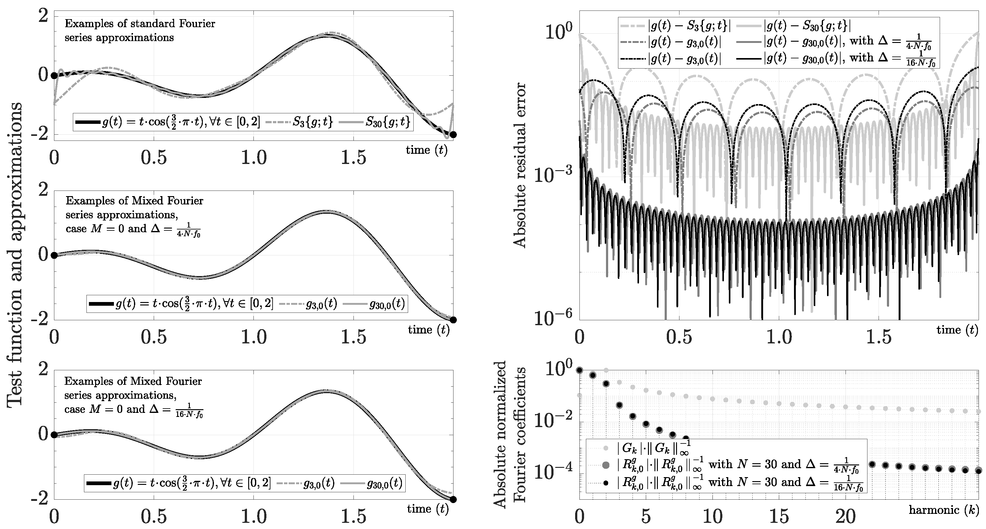
3.2.1. Generic Sawtooth Function

We define this function by

$$g\left(t\right)=\alpha +\beta ·t,\forall t\in [0,T],$$

where $\alpha ,\beta \in \mathbb{R}.$ The coefficients of $S_N\{g;t\}$ are

$$G_k=\left\{\begin{array}{cc}\alpha +\frac{1}{2}·T·\beta \hfill & ,k=0\hfill \\ -\frac{T·\beta }{2\pi i·k}\hfill & ,\forall k\in \mathbb{Z}-\left\{0\right\}\hfill \end{array}\right..$$

(55)

Using $M=0$, we obtain $g\left(0\right)=\alpha$, $g\left(T\right)=\alpha +\beta ·T$. Consequently, $P_{1,0}^g=\beta ·T$ and

$$\begin{array}{cc}\hfill P_0\{g;t\}& =\beta ·t,\forall t\in [0,T],\hfill \end{array}$$

(56)

$$\begin{array}{cc}\hfill R_{k,0}^g& =\alpha ·\mathrm{sinc}\left(k\right)=\left\{\begin{array}{cc}\alpha \hfill & ,k=0\hfill \\ 0\hfill & ,\mathrm{elsewhere}\hfill \end{array}\right..\hfill \end{array}$$

(57)

As expected, we obtain the best possible scenario because only two coefficients (i.e., $P_{1,0}^g=\beta ·T$ and $R_{0,0}^g=\alpha$) are necessary to model this function without errors. From Corollary 1, we obtain $P_{M\ge 0}\{g;t\}=\beta ·t,\forall t\in [0,T]$.

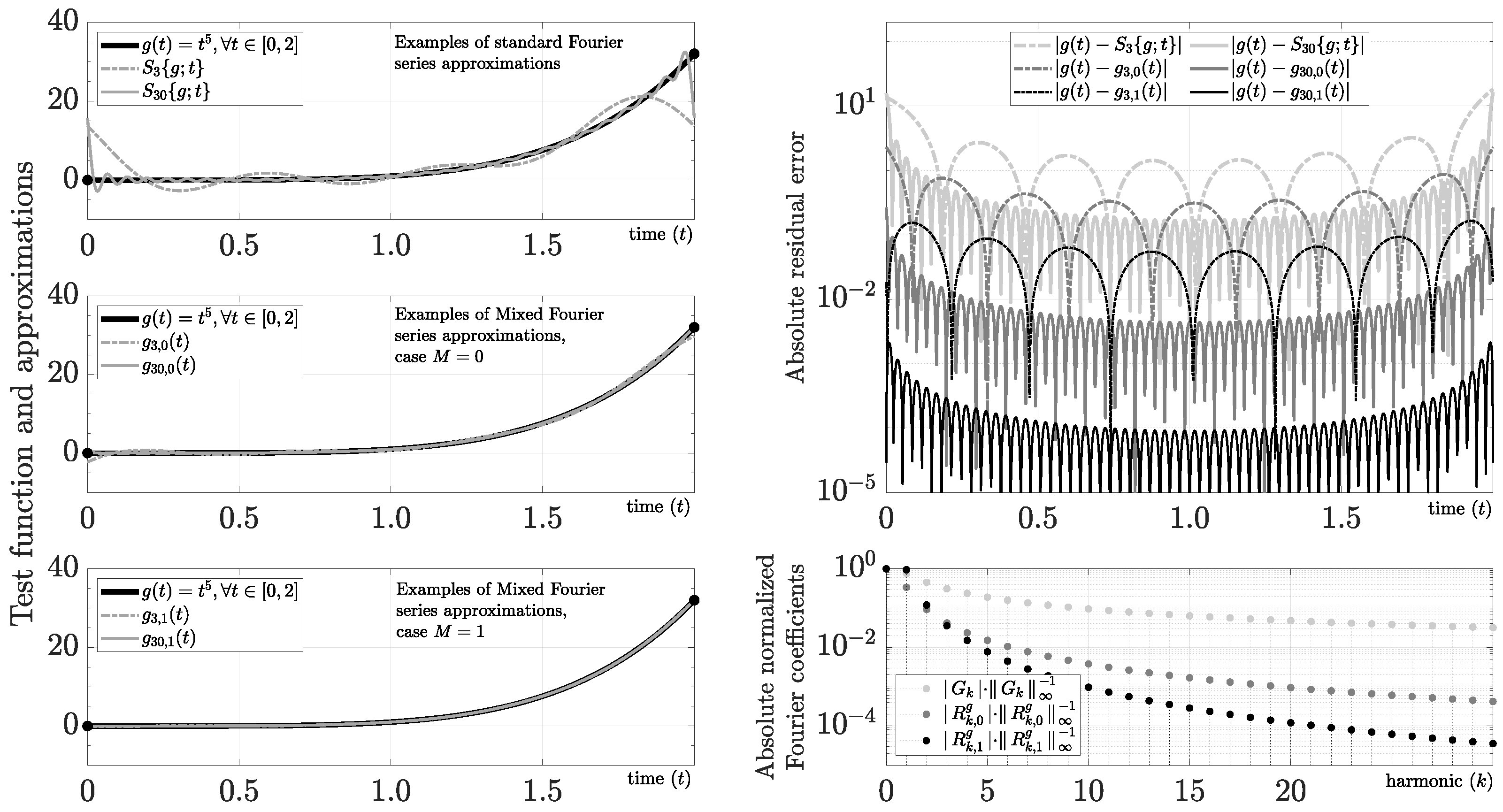
3.2.2. Power Function

We define this function by

$$g\left(t\right)=t^m,\forall t\in [0,T],$$

where $m\in \mathbb{N}-\left\{1\right\}$. The coefficients of $S_N\{g;t\}$ are

$$G_k=\left\{\begin{array}{cc}\frac{1}{m+1}·T^m\hfill & ,k=0\hfill \\ T^m·H_{k,m}\hfill & ,\mathrm{elsewhere}\hfill \end{array}\right..$$

(58)

We are interested in this case because many functions can have partial Taylor approximations. As a result, the ability to approximate polynomials with the mixed series can arise as a relevant question. This function produces ringing artifacts in $S_N\{g;t\}$ for higher values of $m·T^{m-1}$ caused by the change in amplitude and slope at edges. In Figure 2, we show the Fourier series for $m=5$ and $T=2$ using $N=3$ and $N=30$.

In this case, the polynomial constants (31)–(33) use

$$g^{\left(k\right)}\left(t\right)=\left\{\begin{array}{cc}\frac{m!}{(m-k)!}·t^{m-k}\hfill & ,k\le m,\forall t\in [0,T]\hfill \\ 0\hfill & ,k>m,\forall t\in [0,T]\hfill \end{array}\right..$$

(59)

For instance, for $m=5$ and $T=2$, we obtain the following polynomials:

$$\begin{array}{cc}\hfill P_0\{g;t\}& =16t,\forall t\in [0,2],\hfill \end{array}$$

(60)

$$\begin{array}{cc}\hfill P_1\{g;t\}& =20t^2-24t,\forall t\in [0,2],\hfill \end{array}$$

(61)

and using (37) and (45), we obtain the Fourier coefficients

$$\begin{array}{cc}\hfill R_{k,0}& =\left\{\begin{array}{cc}-\frac{32}{3}\hfill & ,k=0\hfill \\ 2^5·H_{k,5}+2^5\frac{1}{2\pi ik}\hfill & ,\mathrm{elsewhere}\hfill \end{array}\right.,\hfill \end{array}$$

(62)

$$\begin{array}{cc}\hfill R_{k,1}& =\left\{\begin{array}{cc}\frac{8}{3}\hfill & ,k=0\hfill \\ R_{k,0}-2^5\frac{5}{{\left(2\pi k\right)}^2}\hfill & ,\mathrm{elsewhere}\hfill \end{array}\right..\hfill \end{array}$$

(63)

As we show in Figure 2, the approximations $g_{N,0}\left(t\right)$ and $g_{N,1}\left(t\right)$ do not have the Gibbs phenomenon, and we obtain control of the decreasing rate of the Fourier coefficients. For instance, we find that the 30th harmonic has $|G_{30}|·{\Vert G_k\Vert }_{\infty }^{-1}$∼$3.1\times {10}^{-2}$ and $|R_{30,M}^g|·{\Vert R_{k,M}^g\Vert }_{\infty }^{-1}$∼$3.5\times {10}^{-5}$ for $M=1$ in this example. As a result, the increase in resolution using the mixed Fourier series is nearly cubic (29.47 dB) for that harmonic. If $M\ge m-1$, then we obtain again the best possible scenario because $P_{M\ge m-1}\{g;t\}=t^m,\forall t\in [0,T]$. Applying superposition, it follows that arbitrary polynomials with degree D have an exact representation when $M\ge D-1$. We emphasize, however, that by using a low-order value of M in the mixed Fourier series, we can avoid using high-order derivatives.

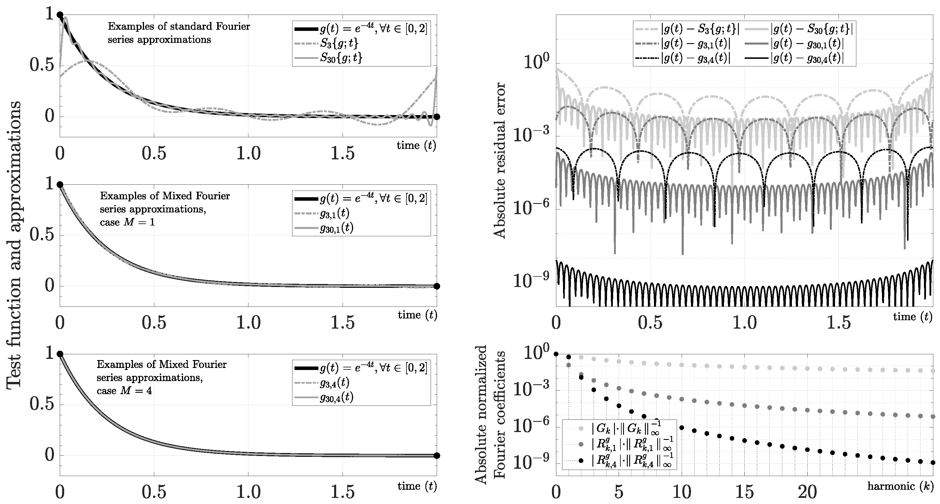
3.2.3. Exponential Function

We define this function by

$$g\left(t\right)=e^{\alpha ·t},\forall t\in [0,T],$$

(64)

where $\alpha \in \mathbb{R}-\left\{0\right\}$. The coefficients of $S_N\{g;t\}$ are

$$G_k=\frac{e^{T\alpha }-1}{T\alpha -2i\pi k},\forall k\in \mathbb{Z}.$$

(65)

This function is of our interest because it could increase or decrease its values very fast. In Figure 3, we show the Fourier series for $\alpha =-4$ and $T=2$ using $N=3$ and $N=30$.

In this case, the polynomial constants (31)–(33) use

$$g^{\left(k\right)}\left(t\right)={\alpha }^k·e^{\alpha ·t},\forall t\in [0,T].$$

(66)

For instance, for $\alpha =-4$ and $T=2$, we obtain the following polynomials:

$$\begin{array}{cc}\hfill P_1\{g;t\}& =-\left(e^{-8}-1\right)\left(t^2-\frac{5}{2}t\right),\forall t\in [0,2],\hfill \end{array}$$

(67)

$$\begin{array}{cc}\hfill P_4\{g;t\}& =\left(e^{-8}-1\right)\sum _{m=1}^5{\varphi }_m·t^m,\forall t\in [0,2],\hfill \end{array}$$

(68)

where ${\varphi }_1=\frac{209}{90}$, ${\varphi }_2=-\frac{31}{3}$, ${\varphi }_3=\frac{124}{9}$, ${\varphi }_4=-\frac{20}{3}$, and ${\varphi }_5=\frac{16}{15}$. On the other hand, the Fourier coefficients $R_{k,M}$ can be calculated efficiently using Corollary 3. In particular, for this example, we find

$$\begin{array}{cc}\hfill R_{k,1}& =\left\{\begin{array}{cc}-\frac{31}{24}\left(e^{-8}-1\right)\hfill & ,k=0\hfill \\ \frac{T\alpha }{(2\pi i·k)}\left(\frac{e^{T\alpha }-1}{T\alpha -2i\pi k}+\frac{e^{T\alpha }-1}{2\pi i·k}\right)\hfill & ,\mathrm{elsewhere}\hfill \end{array}\right.,\hfill \end{array}$$

(69)

$$\begin{array}{cc}\hfill R_{k,4}& =\left\{\begin{array}{cc}-\frac{209}{360}\left(e^{-8}-1\right)\hfill & ,k=0\hfill \\ \frac{T^4{\alpha }^4}{{(2\pi i·k)}^4}\left(\frac{e^{T\alpha }-1}{T\alpha -2i\pi k}+\frac{e^{T\alpha }-1}{2\pi i·k}\right)\hfill & ,\mathrm{elsewhere}\hfill \end{array}\right..\hfill \end{array}$$

(70)

As Figure 3 makes clear, we are able to recover an approximation of this function with $\Vert {g\left(t\right)-g_{3,4}\left(t\right)\Vert }_{\infty }$∼${10}^{-8}$ using 30 harmonics (i.e., $N=30$). From a practical point of view, for $M=4$, we obtain a worst absolute error of ∼${10}^{-3}$ and ∼${10}^{-6}$ using only 3 and 10 harmonics, respectively. For instance, we find that the 30^th harmonic has $|G_{30}|·{\Vert G_k\Vert }_{\infty }^{-1}$∼$4.2\times {10}^{-2}$ and $|R_{30,M}^g|·{\Vert R_{k,M}^g\Vert }_{\infty }^{-1}$∼$1.2\times {10}^{-9}$ for $M=4$ in this example. As a result, the increase in resolution using the mixed Fourier series is almost $75.44$ dB for that harmonic.

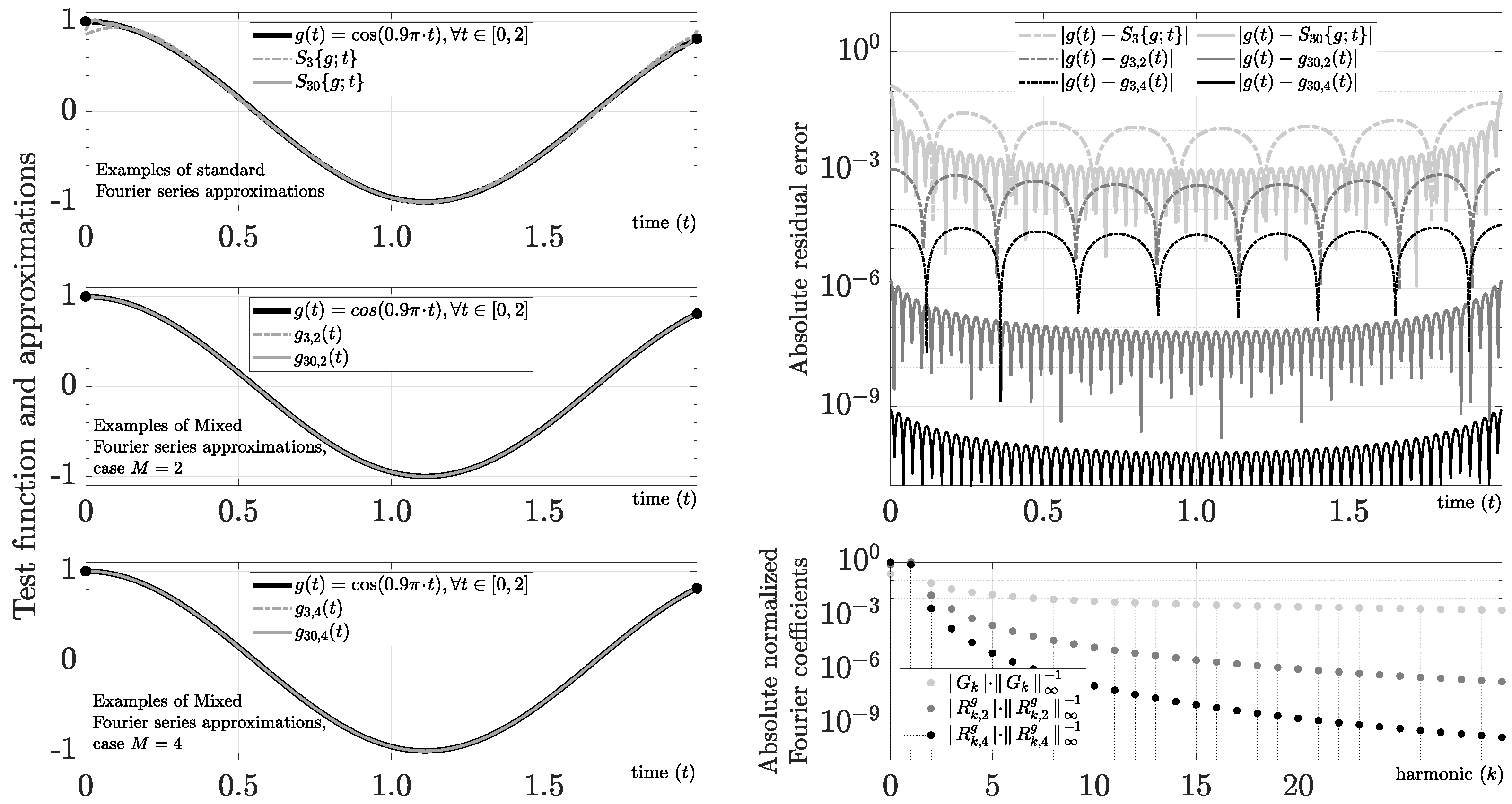
3.2.4. Base-Band Cosine Function

We define this function by

$$g\left(t\right)=cos(2\pi \frac{\beta }{T}·t),\forall t\in [0,T],$$

where $0<\beta <1$. The coefficients of $S_N\{g;t\}$ are

$$G_k=\frac{1}{2}{e}^{-i\pi (k-\beta )}\mathrm{sinc}(k-\beta )+\frac{1}{2}{e}^{-i\pi (k+\beta )}\mathrm{sinc}(k+\beta ).$$

(71)

This function is of our interest because it allows us to study the spectrum leakage in trigonometric base-band functions. As Figure 4 makes clear, even though the Fourier series obtains a small Gibbs phenomenon for $\beta =0.9$ and $T=2$, the spectrum leakage could be relevant for many practical applications.

In this case, the polynomial constants (31)–(33) use

$$g^{\left(k\right)}\left(t\right)={(2\pi \frac{\beta }{T})}^k\left\{\begin{array}{cc}{(-1)}^{\frac{k}{2}+\frac{1}{2}}·sin(2\pi \frac{\beta }{T}·t)\hfill & ,\forall k\in \{1,3,5,\cdots \},\forall t\in [0,T]\hfill \\ {(-1)}^{\frac{k}{2}}·cos(2\pi \frac{\beta }{T}·t)\hfill & ,\forall k\in \{0,2,4,\cdots \},\forall t\in [0,T]\hfill \end{array}\right.,$$

(72)

where the Fourier coefficients $R_{k,M}^g$ can be calculated efficiently using Corollary 3. As an example, for $\beta =0.9$ and $T=2$, we find the following Fourier coefficients:

$$\begin{array}{cc}\hfill R_{k,2}^g& =\left\{\begin{array}{cc}0.268535523631802\hfill & ,k=0\hfill \\ -{\left(\frac{0.9}{ik}\right)}^2\left(G_k+\frac{\{cos(1.8\pi )-1\}}{2\pi ik}\right)\hfill & ,\mathrm{elsewhere}\hfill \end{array}\right.,\hfill \end{array}$$

(73)

$$\begin{array}{cc}\hfill R_{k,4}^g& =\left\{\begin{array}{cc}0.416158284137357\hfill & ,k=0\hfill \\ {\left(\frac{0.9}{ik}\right)}^4\left(G_k+\frac{\{cos(1.8\pi )-1\}}{2\pi ik}\right)\hfill & ,\mathrm{elsewhere}\hfill \end{array}\right..\hfill \end{array}$$

(74)

As expected, Figure 4 shows a reduction in spectral leakage by increasing M. In contrast to the spectral distortion caused by improving amplitude-based frequency discrimination using the Windowing technique, the mixed Fourier series improves amplitude-based frequency discrimination only by increasing M (i.e., without adding artificial distortion). For instance, using a criteria of ${10}^{-2}$ in amplitude-based frequency discrimination, $|G_k|·{\Vert G_k\Vert }_{\infty }^{-1}\ge {10}^{-2}$ requires eight harmonics in Figure 4. In contrast, $|R_{k,M}^g|·{\Vert R_{k,M}^g\Vert }_{\infty }^{-1}\ge {10}^{-2}$ requires only three and two harmonics using $M=2$ and $M=4$, respectively. Using more selective criteria of ${10}^{-3}$ in this example, the standard Fourier approach requires 65 harmonics, and the mixed Fourier series requires 4 and 3 harmonics using $M=2$ and $M=4$, respectively. Nonetheless, a redefinition of $P_M\{g;t\}$ is required to apply this technique directly to carrier detection (i.e., $\beta \gg 1$) because $P_M\{g;t\}$ composed only of polynomials is a base-band function.

3.3. Comparison with Selected State-of-the-Art Techniques

In this subsection, we compare the performance of the mixed Fourier series with other types of series in a variety of scenarios using convenient test functions. Although the term “convenient function” is debatable, we define it as a function that is demanding enough for trigonometric and polynomial basis functions on $[0,T]$ and, at the same time, has a simple mathematical structure that allows us to avoid debating its influence on the numerical implementation. For this reason, we start our comparison with the exponential function previously studied in Section 3.2.3.

Figure 5 shows the performance of the most common averaging and filtering techniques for $N=10$ [27,32], where $F_N\{g;t\}$ is the partial Fejér’s series (i.e., Fejér’s arithmetic mean method), given by

$$F_N\{g;t\}:=\frac{1}{N+1}\sum _{m=0}^N{S}_m\{g;t\},$$

(75)

and ${\sigma }_{N,M}\{g;t\}$ is a partial Fourier series using a particular ${\sigma }_l$-filter with the Mth order, given by

$${\sigma }_{N,M}\{g;t\}:=\sum _{k=-N}^N{G}_k·e^{2\pi i·t·k{f}_0}·{\sigma }_l^{M+1}\left(k·N^{-1}\right).$$

(76)

For example, the standard Lanczos filter (also known as $\sigma$-approximation) is given by ${\sigma }_1\left(x\right)=\mathrm{sinc}\left(x\right):=\frac{sin\left(\pi x\right)}{\pi x}$, the Raised cosine filter is given by ${\sigma }_2\left(x\right):=\frac{1}{2}\{1+cos\left(\pi x\right)\}$, and the Sharpened Raised cosine filter is given by ${\sigma }_3\left(x\right):={\sigma }_2^4\left(x\right)·\{35-84·{\sigma }_2\left(x\right)+70·{\sigma }_2^2\left(x\right)-20·{\sigma }_2^3\left(x\right)\}$. As can be concluded from a cursory examination of Figure 5, we obtain better performance using $g_{N,0}\left(t\right)$. Because the average and convolution operators are smooth operators, methods based on them converge more slowly than $g_{N,M\ge 1}\left(t\right)$.

On the other hand, a comparison between mixed Fourier series and orthogonal polynomials is also pertinent. Figure 6 shows the absolute residual error using the Legendre orthogonal polynomials, denoted by $W_M^{Leg}\{g;t\}$, and the Chebyshev orthogonal polynomials, denoted by $W_M^{Che}\{g;t\}$, both defined on $[0,T]$. As the figure makes clear, both approximations have good performance for $M=10$, where ${\Vert g\left(t\right)-W_M^{Leg}\{g;t\}\Vert }_{\infty }\simeq 9.2\times {10}^{-6}$ and ${\Vert g\left(t\right)-W_M^{Che}\{g;t\}\Vert }_{\infty }\simeq 3.1\times {10}^{-6}$. We are interested in determining some fair comparatives because the mixed Fourier series has two degrees of freedom (i.e., N and M). For instance, we obtain ${\Vert g\left(t\right)-g_{N,10}\left(t\right)\Vert }_{\infty }\le 2.7\times {10}^{-7}$ for $N\ge 3$, which implies that we can improve both orthogonal polynomials by combining simple polynomials with the same degree and a few harmonics from the residual. As another example, we find ${\Vert g\left(t\right)-g_{10,M}\left(t\right)\Vert }_{\infty }\le 1.6\times {10}^{-6}$ for $M\ge 4$, which implies that the same number of unknown harmonics can also improve both orthogonal polynomials using low-order derivatives from the edges. Finally, we obtain ${\Vert g\left(t\right)-g_{6,5}\left(t\right)\Vert }_{\infty }\simeq 2.7\times {10}^{-6}$ such that $min\{M+N\}$, which implies that the mixed Fourier series has a better performance using at least 19 unknown variables (i.e., $M+2N+2$ unknown variables) versus the 11 unknown variables (i.e., $M+1$ unknown variables) from the orthogonal polynomials. In summary, the mixed Fourier series outperforms orthogonal polynomials in several ways. First, we have an additional degree of freedom that has a significant impact on convergence. Second, we have less computational complexity because the interior product is more simple and computationally efficient using the Fourier approach (i.e., $G_k$ can be defined in terms of an inner product using the same framework of orthogonal polynomials). Third, our approach implies uniform sampling, which simplifies the numerical implementation using the $\mathrm{DFT}\{·\}$. Finally, we also find a quasi-spectral accuracy because $|R_{N,M}^g|\le D_{max}·{\left|N\right|}^{-M}$, where $M\le K$ and $D_{max}$ is (47).

Another critical situation to discuss is when the Taylor series of $g\left(t\right)$ at $t_0$, defined by $T_M\{g;t;t_0\}:={\sum }_{k=0}^M\frac{1}{k!}{g}^{\left(k\right)}\left(t_0\right){(t-t_0)}^k$, cannot converge in the whole domain or at some point of the domain (e.g., $g\left(t\right)$ is a smooth function but a non-analytic function at some $t_0\in [0,T]$). For instance, the case $g\left(t\right)=ln(t+1),\forall t\in [0,2]$, allows us to discuss a typical example where the Taylor series cannot converge in the whole domain using $t_0=0$ because its residual has a region of convergence $\left|t\right|<1$, as we show in Figure 7. As happens in this example, the mixed Fourier series can be found by using a mixed evaluation (i.e., a combination of closed-form and numerical evaluations). On the one hand, we can usually find $P_{m,M}^g$ from closed-form derivatives, as shown in this example by

$$g^{\left(k\right)}\left(t\right)=\left\{\begin{array}{cc}ln(t+1)\hfill & k=0,\forall t\in [0,T]\hfill \\ -\frac{{(-1)}^k·(k-1)!}{{(t+1)}^k}\hfill & k\in \mathbb{N},\forall t\in [0,T]\hfill \end{array}\right.$$

(77)

On the other hand, because closed-form Fourier coefficients are relatively uncommon for many well-known functions, we can approximate $G_k\approx {\mathcal{T}}_N\{{\widehat{G}}_k\}$ and $R_{k,M}^g\approx {\mathcal{T}}_N\{{\widehat{R}}_{k,M}^g\}$ using the Discrete Fourier Transform (DFT) of $2N+1$ points through

$${\mathcal{T}}_N\{{\widehat{G}}_k\}:=\frac{1}{2N+1}·\left\{\begin{array}{cc}{\widehat{G}}_0\hfill & ,k=0\hfill \\ {\widehat{G}}_k\hfill & ,\forall k\in [1,N]\hfill \\ {\widehat{G}}_{2N+k+1}\hfill & ,\forall k\in [-N,-1]\hfill \end{array}\right.,$$

(78)

where

$${\widehat{G}}_k=\mathrm{DFT}{\left\{g\left(t_n\right)\right\}}_{n=0}^{2N}:=\sum _{n=0}^{2N}g\left(t_n\right)·e^{-\frac{2\pi }{2N+1}i·kn},\forall k\in [0,2N]$$

(79)

and

$$\begin{array}{cc}\hfill {\widehat{R}}_{k,M}^g& :=\mathrm{DFT}{\{g\left(t_n\right)-P_M\{g;t_n\}\}}_{n=0}^{2N}\hfill \end{array}$$

(80)

using the uniform samples $t_n=h·n,\forall n\in \{0,1,\cdots ,2N\}$, and $h=\frac{T}{2N+1}$. According to the Sampling Theory [113,114], this approach converges by increasing N because the aliasing from the discrete-time model is removed when $N\to \infty$ for $g\in {\mathcal{C}}^K[0,T]$. In particular, because $ln(·)$ does not have closed-form Fourier coefficients, we can use (80) to obtain $g_{N,M}\left(t\right)$. As shown in Figure 7, the mixed evaluation allows us to obtain a convergent approximation for increasing values of M and N. Similarly, another relevant case study is given by $g\left(t\right)=e^{-1/t^2},\forall t\in (0,2]$ and $g\left(0\right)=0$ because it is a typical smooth function with non-analytic behavior at $t_0=0$ (i.e., caused by $g^{\left(k\right)}\left(0\right)=0,\forall k\in \mathbb{N}\cup \left\{0\right\}$). As we show in Figure 7, we also obtain a convergent mixed Fourier series for increasing values of M and N.

Lastly, it is pertinent to evaluate this mixed evaluation with special cases, for example, when the test function exhibits both Gibbs and Runge’s phenomena. In particular, we propose the study case $g\left(t\right)=tanh(\alpha ·t-\frac{1}{2}\alpha ·T),\forall t\in [0,T]$, using $\alpha =4$ and $T=2$. As shown in Figure 8, we obtain Runge’s phenomenon by using a partial interpolating polynomial series $L_{2N+1}\{g;t\}={\sum }_{m=0}^{2N+1}{\alpha }_m·{\left(\frac{t}{T}\right)}^m$ and uniform matching nodes $t_n=h·n,\forall n\in \{0,1,\cdots ,2N+1\}$. On the other hand, we obtain the Gibbs phenomenon by using a partial Fourier interpolating series $S_N\{g;t\}={\sum }_{k=-N}^N{G}_k·e^{2\pi i·t·k{f}_0}$, where $G_k$ is approximated by ${\mathcal{T}}_N\{{\widehat{G}}_k\}$ with uniform matching nodes $t_n=h·n,\forall n\in \{0,1,\cdots ,2N\}$. One well-known solution for this situation is obtained by using nonuniform sampling, for example, with the Chebyshev interpolating function $T_{2N+1}\{g;t\}={\sum }_{m=0}^{2N+1}{\beta }_m·T_m(\frac{2}{T}t-1)$ and the Chebyshev–Gauss–Lobatto (CGL) matching nodes given by $t_l:=\frac{T}{2}\{1+cos(\frac{l·\pi }{2N+1})\},$$\forall l\in \{0,\cdots ,2N+1\}$ [115]. In this paper, we propose a different solution obtained by $g_{N,1}\left(t\right)$ using uniform matching nodes $t_n=h·n,\forall n\in \{0,1,\cdots ,2N\}$, ${\mathcal{T}}_N\{{\widehat{R}}_{k,1}^g\}$, and

$$P_1\{g;t\}=2·tanh(\frac{1}{2}\alpha ·T)·\left(\frac{t}{T}\right),\forall t\in [0,T].$$

(81)

Despite the reduced performance due to the mixed evaluation, Figure 8 shows that $g_{N,1}\left(t\right)$ has the best performance without Gibbs and Runge’s phenomena, outperforming the Chebyshev interpolating function. For instance, we obtain an absolute residual error around ${\Vert g\left(t\right)-g_{7,1}\left(t\right)\Vert }_{\infty }$∼$1.5\times {10}^{-4}$ using seven harmonics (i.e., $N=7$). If we increase $\alpha$, then more harmonics (and samples) will be necessary for a good approximation because the test function increases its bandwidth.

Although the Legendre, Chebyshev, or other modern interpolating series may perform better for other smooth functions, we have shown in several situations that the mixed Fourier series allows us to interpolate a closed-form function without anomalous phenomena caused by convergence. Unlike interpolating methods such as Legendre and Chebyshev, the method for finding $g_{N,M}\left(t\right)$ is well conditioned because the DFT is well conditioned and the polynomial constants are found using a low-cost backward algorithm. In summary, we can derive a mixed Fourier series from a closed-form evaluation of $g\left(t\right)$ or from a mixed evaluation of $g\left(t\right)$, where the new series may outperform common signal presentations with low complexity and well-conditioned methodologies. The Maliev–Lanczos approach has two degrees of freedom, which allows quasi-spectral accuracy. Moreover, it has a simple method based on uniform sampling with convergence everywhere for $M\ge 1$, which allows us to avoid Gibbs and Runge phenomena for $g\in {\mathcal{C}}^{K\ge 1}[0,T]$.

3.4. A Canonical Direct Problem: Numerical Riemann Integration of Closed-Form Smooth Functions

Numerical integration using uniform samples has several advantages because of its computational simplicity. Because the magnitude of Fourier coefficients of $\overline{r}\in C^M\left(\mathbb{R}\right)$ has the property $O({\left|k\right|}^{-M})$, it is a reasonable hypothesis that $r\left(t\right)$ allows better numerical integration using the Newton–Cotes quadrature rules [116]. Therefore, we propose the numerical integration of $g\left(t\right)$ using $r(t$) by means of

$$\begin{array}{cc}\hfill I={\int }_0^{T}g\left(t\right)dt& ={\int }_0^T\left(P_M\{g;t\}+r\left(t\right)\right)dt\hfill \\ \hfill & \approx T·\sum _{m=1}^{M+1}\frac{1}{m+1}·P_{m,M}^g+\sum _{n=0}^{2N+1}{w}_n·r\left(t_n\right),\hfill \end{array}$$

(82)

where $h=T/(2N+1)$, $t_n=n·h$, $r\left(t_n\right)=g\left(t_n\right)-P_M\{g;t_n\}$, and $w_n$ denotes the weights for a particular quadrature rule [116].

As a case of study, we evaluate $I={\int }_0^3{e}^{-t^2}dt$ in Figure 9 by means of the absolute relative error of the integral defined by $\eta :=\left|1-\frac{I_{approx}}{I_{exact}}\right|$. We compare (82) with

$${\int }_0^{T}g\left(t\right)dt\approx \sum _{n=0}^{2N+1}{w}_n·g\left(t_n\right)$$

(83)

using the left rectangular rule (i.e., left Riemann sums), the trapezoidal rule, and Simpson’s rule. As we show in this example, the simple left rectangular rule (i.e., $w_n=h,\forall n\in [0,2N]$ and $w_{2N+1}=0$) obtains a higher performance. For instance, Figure 9 shows that using that simplest integration scheme, the evaluation of (82) only requires $N>10$ with $M=3$ for a typical relative integration error of $1\times {10}^{-10}$. This result makes sense using the Fourier framework because $r\left(t_n\right)$ has less aliasing than its counterpart $g\left(t_n\right)$.

3.5. A Canonical Inverse Problem: Solution of a Boundary Value Problem (BVP) Using Standard Closed-Form Fourier Coefficients

The mixed Fourier series emerged when we were analyzing the solution of Poisson’s equation in one dimension with a Dirichlet boundary condition using the Fourier series [117]. Our approach to solving that problem is as follows.

Let $x\in {\mathcal{C}}^2[0,T]$ be an unknown function such that

$$\begin{array}{cc}\hfill \frac{d^2}{d{t}^2}x(t)& =\lambda ·y\left(t\right),\forall t\in [0,T],\hfill \end{array}$$

(84)

$$\begin{array}{cc}\hfill \mathrm{s}.\mathrm{t}.& x\left(0\right),x\left(T\right)\in \mathbb{R}\hfill \end{array}$$

(85)

where we use the right-hand derivative definition at $t=0$, the left-hand derivative definition at $t=T$, and $\lambda \in \mathbb{R}$.

If we assume that $y\in {\mathcal{C}}^0[0,T]$ has a partial Fourier series given by

$$S_N\{y;t\}=\sum _{k=-N}^N{Y}_k·e^{2\pi i·t·k{f}_0},\forall t\in [0,T],$$

(86)

such that $|Y_k|$ is $O({\left|k\right|}^{-1})$, then the partial series solution of this problem is

$$x_{N,1}\left(t\right)=\sum _{k=-N}^N{R}_{k,1}^x·e^{2\pi i·t·k{f}_0}+\sum _{m=1}^2{P}_{m,1}^x·{\left(\frac{t}{T}\right)}^m,\forall t\in [0,T].$$

(87)

Replacing $x_{N,1}\left(t\right)$ and $S_N\{y;t\}$ in (84), and using the boundaries and the orthogonality of the harmonics, we obtain

$$\begin{array}{cc}\hfill R_{k,1}^x& =\frac{\lambda }{{(2\pi i·k{f}_0)}^2}·Y_k,\forall k\in \{\pm 1,\cdots ,\pm N\},\hfill \end{array}$$

(88)

$$\begin{array}{cc}\hfill R_{0,1}^x& =x\left(0\right)-2·\sum _{k=1}^N\mathrm{Re}\left\{R_{k,1}^x\right\},\hfill \end{array}$$

(89)

$$\begin{array}{cc}\hfill P_{2,1}^x& =\frac{\lambda }{2}·T^2·Y_0,\hfill \end{array}$$

(90)

$$\begin{array}{cc}\hfill P_{1,1}^x& =\{x\left(T\right)-x\left(0\right)\}-P_{2,1}^x.\hfill \end{array}$$

(91)

This result is always convergent because $y\left(t\right)$ is bounded by the Boundedness Theorem, $|Y_k|$ has a decreasing rate $O({\left|k\right|}^{-1})$ [24], and $|R_{k,1}^x|$ has a decreasing rate $O({\left|k\right|}^{-3})$. Therefore, ${\sum }_{k=1}^{\infty }\mathrm{Re}\{R_{k,1}^x\}$ is bounded, too.

In particular, if $x\left(t\right)=sin\left(t\right),\forall t\in [0,\frac{\pi }{2}]$, and $\lambda =-1$, then $y\left(t\right)=sin\left(t\right),\forall t\in [0,\frac{\pi }{2}]$, and

$$Y_k=\frac{2}{\pi }·\frac{4ik-1}{16k^2-1}.$$

(92)

In this case, we can see that there are two types of series for the same function $x\left(t\right)=y\left(t\right)=sin\left(t\right),\forall t\in [0,\frac{\pi }{2}]$. The first is the standard partial Fourier series using the coefficients (92), which have a decreasing rate $O({\left|k\right|}^{-1})$, and they produce ringing artifacts, as shown in Figure 10. The second is a mixed Fourier series using particular coefficients with $x\left(0\right)=0$ and $x\left(T\right)=1$ obtained from the BVP by (88)–(91). The mixed series includes Fourier coefficients with a decreasing rate $O({\left|k\right|}^{-3})$, and they do not produce ringing artifacts, as shown in Figure 10. These characteristics motivated us to develop an in-depth analysis of this series and its applications in the framework of signal processing, which is described in this paper.

On the other hand, the solution using the mixed series has better accuracy compared with the standard Finite Difference Method (FDM) [118] given by

$$\left[\begin{array}{cccccc}-2& 1& & & & \\ 1& -2& 1& & & \\ & & \ddots & \ddots & \ddots & \\ & & & 1& -2& 1\\ & & & & 1& -2\end{array}\right]\left[\begin{array}{c}{x}_{2N}\left(t_1\right)\\ x_{2N}\left(t_2\right)\\ ⋮\\ x_{2N}\left(t_{2N-1}\right)\\ x_{2N}\left(t_{2N}\right)\end{array}\right]=\lambda ·h^2\left[\begin{array}{c}y\left(t_1\right)\\ y\left(t_2\right)\\ ⋮\\ y\left(t_{2N-1}\right)\\ y\left(t_{2N}\right)\end{array}\right]-\left[\begin{array}{c}x\left(0\right)\\ 0\\ ⋮\\ 0\\ x\left(T\right)\end{array}\right],$$

(93)

where $h=T/(2N+1)$ and $t_n=n·h,\forall n\in [1,2N]$. Furthermore, the complexity to find the unknown constants in both cases is $O\left(N\right)$ because the solution of (93) using the tridiagonal matrix algorithm is $O\left(N\right)$, the evaluation of (88) or (89) is $O\left(N\right)$, and the evaluation of (90) or (91) is $O\left(1\right)$. Figure 10 shows the FDM solution using linear interpolation, too.

Finally, we can still improve the accuracy of Poisson’s Equation solution for any $y\in {\mathcal{C}}^0[0,T]$ using $y_{N,0}\left(t\right)$ and $x_{N,2}\left(t\right)$, where

$$\begin{array}{cc}\hfill R_{k,0}^y& =\left\{\begin{array}{cc}{Y}_0-\frac{1}{2}\{y\left(T\right)-y\left(0\right)\}\hfill & k=0\hfill \\ Y_k+\frac{\left\{y\right(T)-y(0\left)\right\}}{2\pi i·k}\hfill & \mathrm{elsewhere}\hfill \end{array}\right.,\hfill \end{array}$$

(94)

$$\begin{array}{cc}\hfill R_{k,2}^x& =\frac{\lambda }{{(2\pi i·k{f}_0)}^2}·R_{k,0}^y,\forall k\in \{\pm 1,\cdots ,\pm N\},\hfill \end{array}$$

(95)

$$\begin{array}{cc}\hfill R_{0,2}^x& =x\left(0\right)-2·\sum _{k=1}^N\mathrm{Re}\left\{R_{k,2}^x\right\},\hfill \end{array}$$

(96)

$$\begin{array}{cc}\hfill P_{3,2}^x& =\frac{\lambda }{6}·T^2·(y\left(T\right)-y\left(0\right)),\hfill \end{array}$$

(97)

$$\begin{array}{cc}\hfill P_{2,2}^x& =\frac{\lambda }{2}·T^2·R_{0,0}^y,\hfill \end{array}$$

(98)

$$\begin{array}{cc}\hfill P_{1,2}^x& =x\left(T\right)-x\left(0\right)-P_{2,2}^x-P_{3,2}^x.\hfill \end{array}$$

(99)

Figure 10 also shows the solution using $x\left(T\right)=y\left(T\right)=1$ and $x\left(0\right)=y\left(0\right)=0$, where ${\Vert x\left(t\right)-x_{3,2}\left(t\right)\Vert }_{\infty }\sim 6\times {10}^{-5}$ is obtained using only three harmonics (i.e., $N=3$).

3.6. A Canonical Inverse Problem: Solution of a Boundary Value Problem (BVP) Using the DFT

In the absence of direct knowledge of the Fourier coefficients of $y\left(t\right)$, we can use the approximation based on the DFT, given by ${\mathcal{T}}_N\{{\widehat{R}}_{k,M}^y\}$, without ambiguities at the edges of the interval because we always obtain ${\overline{r}}_y\in {\mathcal{C}}^M\left(\mathbb{R}\right)$ using the Maliev–Lanczos approach. Furthermore, $P_{m,M}^y$ is obtained from $y\left(t\right)$, and the coefficients $P_{m,M+L}^x$ and $R_{k,M+L}^x$ are obtained from $P_{m,M}^y$ and $R_{k,M}^y$ using the boundaries.

In particular, the case $M=0$ is always relevant because we simplify the formulation without derivatives. For example, in Figure 10, we compare Poisson’s solution using ${\mathcal{T}}_N\{{\widehat{R}}_{k,M}^y\}$ with (95)–(99). As we show, even though the solution loses accuracy in comparison to the theoretical value $R_{k,0}^y$, the residual error is still acceptable in comparison to the other solutions.

3.7. Toward an Ideal Sampling Theorem for Truncated Continuous-Time Functions

Let $g_T:\mathbb{R}\to \mathbb{R}$ be a truncated function defined by

$$g_T\left(t\right)=\left\{\begin{array}{cc}g\left(t\right)\hfill & ,\forall t\in [0,T]\hfill \\ 0\hfill & ,\mathrm{elsewhere}\hfill \end{array}\right..$$

(100)

From the Fourier analysis, it is well known that truncated functions are not band-limited. As a result, sampling that function may result in relevant aliasing when the sampling frequency is reasonably close to twice the usual bandwidth $\left(BW\right)$ definitions, such as half-power bandwidth or first null bandwidth. Using the ideal sampling theorem [113,114], the number of instantaneous samples required to rebuild $g_T:\mathbb{R}\to \mathbb{R}$ using a Fourier approach is asymptotic, and it is given by $\frac{T}{T_s}=\frac{f_s}{f_0}\gg \frac{2BW}{f_0}$. This result implies many samples to rebuild the truncated function for high-resolution applications. The mixed Fourier series provides a method for quantifying the finite number of instantaneous samples required to rebuild $g_T\left(t\right)$ through $g\left(t\right)$ such that $g\in {\mathcal{C}}^M[0,T],\forall M\in \mathbb{N}$. The procedure can be argued as follows:

1.

If ${lim}_{M\to \infty }\left|P_{M+1,M}^g\right|\to 0$, then $\exists M_0\ge 0$ such that ${lim}_{M\to \infty }{P}_M\{g;t\}=P_{M_0}\{g;t\}+{ϵ}_1\left(t\right)$, where ${sup}_{\forall t\in [0,T]}\left|{ϵ}_1\left(t\right)\right|$ can be as small as desired.

2.

If ${lim}_{k,M\to \infty }\left|R_{k,M}^g\right|\to 0$, then $\exists N_0\ge 0$ such that ${lim}_{N,M\to \infty }{R}_{NM}\{r;t\}=R_{N_0}\{r;t\}+{ϵ}_2\left(t\right)$, where ${sup}_{\forall t\in [0,T]}\left|{ϵ}_2\left(t\right)\right|$ can be as small as desired. The bandwidth of $\overline{r}\left(t\right)$ with this approach is $BW=N_0{f}_0$.

3.

Conclusively, if both previous limits converge to zero, then ${lim}_{N,M\to \infty }{g}_{{}_{NM}}\left(t\right)=P_{M_0}\{g;t\}+R_{N_0}\{r;t\}+ϵ\left(t\right)$, where ${sup}_{\forall t\in [0,T]}\left|ϵ\left(t\right)\right|$ can be as small as desired.

Therefore, $2M_0+2$ instantaneous samples from the edges (i.e., $g\left(0\right)$, $g\left(T\right),\cdots$, $g_0^{\left(M_0\right)}\left(0\right),g^{\left(M_0\right)}\left(T\right)$) are required to obtain $P_{M_0}\{g,t\}$, and $2N_0+1$ instantaneous samples related to the periodic residual error (i.e., $r\left(t_i\right)=g\left(t_i\right)-P_{M_0}\{g;t_i\}$, where $t_0=0,\cdots$, $t_{2N_0}=T$) are required to obtain $R_{N_0}\{r;t\}$ by means of DFT. Conclusively, we require at least $2M_0+2N_0+1$ different instantaneous samples from $g\left(t\right)$ and its derivatives to rebuild its form in a finite interval $[0,T]$ with an error as small as desired.

Example 2 (Numerical case).

We studied the exponential function with $\alpha =-4$ and $T=2$ in Section 3.2.3 using the Fourier series and the mixed Fourier series with $M=1$ and $M=4$. First, the Fourier series in this example does not converge to zero using ${sup}_{\forall t\in [0,T]}\left|g\left(t\right)-S_N\{g;t\}\right|$ because it has the Gibbs phenomenon. In contrast, the mixed Fourier series converges with ${sup}_{\forall t\in [0,T]}\left|g\left(t\right)-g_{N,4}\{g;t\}\right|\le {10}^{-11}$ using $N\ge 74$. As a result, our approach for $M=4$ requires at least 149 samples (i.e, $2N+1$) to estimate the Fourier coefficients numerically using the DFT and 10 samples (i.e., $2M+2$) of the $k^{th}$ derivatives at the edges to determine the constants $P_{1,4}^g,\cdots ,P_{5,4}^g$. If we make the same calculation using the Taylor series, then this example requires $M\ge 38$ for $t_0=0$, $M\ge 23$ for $t_0=\frac{T}{2}=1$, and $M\ge 34$ for $t_0=T=2$. As a result, in the best of those cases, the Taylor series with the same error requires 24 samples (i.e., $M+1$) of the $k^{th}$ derivatives at $t_0=\frac{T}{2}=1$. Nevertheless, the cases $M=1$ and $M=4$ using the mixed Fourier series were only included in Section 3.2.3 to compare low-order convergences. If $\mathit{M}:=\left[M_m\right]=\left[\begin{array}{cccccccccccc}1& 2& 3& 4& 5& 6& 7& 8& 9& 10& 11& 12\end{array}\right]$, then the mixed Fourier series converges with the same criterion for $\mathit{N}:=\left[N_m\right]=\left[\begin{array}{cccccccccccc}\mathrm{26,000}& 2800& 380& 74& 54& 32& 20& 16& 11& 9& 8& 7\end{array}\right]$. As can be seen, the number of harmonics does not change significantly when $M_m>8$. In fact, we want to emphasize the limiting factor $N_m+M_m\approx 19$ for $M_m>8$. The major advantage of this approach is given by avoiding the information of higher-order derivatives at one point in the exchange of instantaneous samples in the whole domain. The absolute residual errors for some cases are shown in Figure 11.

Example 3 (Theoretical case).

The exponential function (64) has the following properties: $g^{\left(M\right)}\left(t\right)={\alpha }^{M}g\left(t\right)$, $g\in {\mathcal{C}}^M[0,T]$ for $\forall M\in \mathbb{N}\cup \left\{0\right\}$, and $G_k=\frac{e^{T\alpha }-1}{T\alpha -2i\pi k},\forall k\in \mathbb{Z}$. This function has $P_{M+1,M}^g=\frac{1}{(M+1)!}{\left(T\alpha \right)}^M\{e^{T\alpha }-1\}$ using (31). Therefore, we can choose a finite $M_0>T\left|\alpha \right|$ such that $P_{M_0+1,M_0}^g$ is as small as desired because the factorial grows faster than polynomials and exponentials. On the other hand, we find that $R_{k,M}^g={\left(\frac{T\alpha }{2\pi i·k}\right)}^M(\frac{\{e^{T\alpha }-1\}}{T\alpha -2i\pi k}+\frac{\{e^{T\alpha }-1\}}{2\pi i·k})$ for $\forall k\ne 0$ using (43). Therefore, if $N_0>T·\left|\alpha \right|$, then ${lim}_{M\to \infty }\left|R_{N_0,M}^g\right|\to 0$. Conclusively, using the mixed Fourier series, the number of different instantaneous samples required to rebuild $g\left(t\right)=e^{\alpha t},\forall t\in [0,T]$, with an error as small as desired is $2M_0+2N_0+1$, where $M_0,N_0$ are convenient and bounded constants such that $M_0,N_0>T\left|\alpha \right|$.

3.8. Canonical Example of a Non-Polynomial Mixed Fourier Series: The Sub-Harmonic Case

The methodology utilized in Section 2.2 to obtain the polynomial mixed Fourier series based on the smooth periodic residual error is a framework for defining any mixed Fourier series. In this subsection, we illustrate this methodology to find a novel mixed Fourier series with a non-polynomial form.

Let

$$P_M\{g;t\}=\sum _{m=1}^{\frac{M+1}{2}}{A}_{m,M}^g·cos(2\pi {\widehat{f}}_{m}t)+\sum _{m=1}^{\frac{M+1}{2}}{B}_{m,M}^g·sin(2\pi {\widehat{f}}_{m}t),\forall t\in [0,T]$$

(101)

be a sub-harmonic partial series, where $M\in \mathbb{N}$ is an odd number, ${\widehat{f}}_m\in \mathbb{R}-\{k·f_0\},\forall k\in \mathbb{Z}$, such that $0<{\widehat{f}}_1<\cdots <{\widehat{f}}_{(M+1)/2}$, and $A_{m,M}^g,B_{m,M}^g\in \mathbb{R}$. Let

$$H_{N,M}\{g;t\}:=P_M\{g;t\}+\sum _{k=-N}^N{R}_{k,M}^g·e^{2\pi i·t·k{f}_0},\forall t\in [0,T]$$

(102)

be the sub-harmonic mixed Fourier series, where

$$R_{k,M}^g=G_k+\sum _{m=1}^{\frac{M+1}{2}}{A}_{m,M}^g·\frac{ik·C_m-{\rho }_m·S_m}{2\pi ({\rho }_m^2-k^2)}+\sum _{m=1}^{\frac{M+1}{2}}{B}_{m,M}^g·\frac{ik·S_m+{\rho }_m·C_m}{2\pi ({\rho }_m^2-k^2)},\forall k\in \mathbb{Z},$$

(103)

and ${\rho }_m:=T·{\widehat{f}}_m$, $C_m:=cos\left(2\pi {\rho }_m\right)-1$, and $S_m:=sin\left(2\pi {\rho }_m\right)$.

Because we assume the property $g,r\in {\mathcal{C}}^M[0,T]$, the derivative

$$g^{\left(k\right)}\left(t\right)=r^{\left(k\right)}\left(t\right)+\sum _{m=1}^{\frac{M+1}{2}}{A}_{m,M}^g·\frac{d^k}{d{t}^k}cos(2\pi {\widehat{f}}_{m}t)+\sum _{m=1}^{\frac{M+1}{2}}{B}_{m,M}^g·\frac{d^k}{d{t}^k}sin(2\pi {\widehat{f}}_{m}t)$$

(104)

exists for $\forall t\in [0,T]$ and $\forall k\in \{0,1,\cdots ,M\}$. Because we design $P_M\{g;t\}$ such that the equivalent periodic residual error has a smooth property derived from $r^{\left(k\right)}\left(0\right)=r^{\left(k\right)}\left(T\right)$, the unknown sub-harmonic coefficients (i.e., $A_{m,M}^g$ and $B_{m,M}^g$) can be obtained by

$$\begin{array}{cc}\hfill g^{\left(k\right)}\left(T\right)-g^{\left(k\right)}\left(0\right)& =\sum _{m=1}^{\frac{M+1}{2}}{A}_{m,M}^g·\left(\frac{d^k}{d{t}^k}cos(2\pi {\widehat{f}}_{m}t)\left|{}_{t=T}\right.-\frac{d^k}{d{t}^k}cos(2\pi {\widehat{f}}_{m}t)\left|{}_{t=0}\right.\right)\hfill \\ & +\sum _{m=1}^{\frac{M+1}{2}}{B}_{m,M}^g·\left(\frac{d^k}{d{t}^k}sin(2\pi {\widehat{f}}_{m}t)\left|{}_{t=T}\right.-\frac{d^k}{d{t}^k}sin(2\pi {\widehat{f}}_{m}t)\left|{}_{t=0}\right.\right)\hfill \end{array}$$

(105)

for $\forall k\in \{0,1,\cdots ,M\}.$ For example, if $M=1$, then we obtain

$$\left[\begin{array}{cc}{C}_1& S_1\\ -{\rho }_1·S_1& {\rho }_1·C_1\end{array}\right]\left[\begin{array}{c}{A}_{1,1}^g\\ B_{1,1}^g\end{array}\right]=\left[\begin{array}{c}{F}_0^g\\ {\left(2\pi \right)}^{-1}·F_1^g\end{array}\right],$$

(106)

and if $M=3$, then we obtain

$$\left[\begin{array}{cccc}{C}_1& C_2& S_1& S_2\\ -{\rho }_1·S_1& -{\rho }_2·S_2& {\rho }_1·C_1& {\rho }_2·C_2\\ {\rho }_1^2·C_1& {\rho }_2^2·C_2& {\rho }_1^2·S_1& {\rho }_2^2·S_2\\ -{\rho }_1^3·S_1& -{\rho }_2^3·S_2& {\rho }_1^3·C_1& {\rho }_2^3·C_2\end{array}\right]\left[\begin{array}{c}{A}_{1,3}^g\\ A_{2,3}^g\\ B_{1,3}^g\\ B_{2,3}^g\end{array}\right]=\left[\begin{array}{c}{F}_0^g\\ {\left(2\pi \right)}^{-1}·F_1^g\\ -{\left(2\pi \right)}^{-2}·F_2^g\\ -{\left(2\pi \right)}^{-3}·F_3^g\end{array}\right],$$

(107)

where $F_k^g$ is (33). The matrix formulation for an arbitrary odd case is easily generalized from (105)–(107).

The sub-harmonic mixed Fourier series could have a better performance and versatility than the polynomial mixed Fourier series in several scenarios because it is phenomenologically related to the Fourier basis functions (i.e., it is interpreted literally as a better spectral resolution for some harmonics). Additionally, we can select the sub-harmonics following some special profile for any band-base or pass-band functions. For instance, we can use a uniform distribution (e.g., sub-frequencies ${\widehat{f}}_m\in \{\frac{1}{3}{f}_0,\frac{2}{3}{f}_0\}$ or sub-harmonics ${\rho }_m\in \{\frac{1}{3},\frac{2}{3}\}$), a non-self-interfering but equally spaced distribution (e.g., sub-frequencies ${\widehat{f}}_m\in \{\frac{1}{6}{f}_0,\frac{1}{3}{f}_0\}$ or sub-harmonics ${\rho }_m\in \{\frac{1}{6},\frac{1}{3}\}$), or a particular logarithm distribution (e.g., sub-frequencies ${\widehat{f}}_m\in \{\frac{1}{9}{f}_0,\frac{1}{3}{f}_0\}$ or sub-harmonics ${\rho }_m\in \{\frac{1}{9},\frac{1}{3}\}$) for any band-base function using $M=3$. Many others are possible depending on the characteristic of $g\left(t\right)$ or the conditioning of the matrix resulting from (105).

Although a comprehensive examination of all the characteristics and applications of this new mixed Fourier series is beyond the scope of this paper, we will cover some of them briefly below. First, we obtain the same performance as the polynomial mixed Fourier series when $T·{\widehat{f}}_{(M+1)/2}\ll 1$ because

$$\begin{array}{cc}\hfill cos(2\pi {\widehat{f}}_{m}t)& \approx \sum _{k=0}^{(M+1)/2}\frac{{(-1)}^k}{\left(2k\right)!}{(2\pi {\widehat{f}}_{m}t)}^{2k},\forall t\in [0,T],\hfill \end{array}$$

(108)

$$\begin{array}{cc}\hfill sin(2\pi {\widehat{f}}_{m}t)& \approx \sum _{k=0}^{(M-1)/2}\frac{{(-1)}^k}{(2k+1)!}{(2\pi {\widehat{f}}_{m}t)}^{2k+1},\forall t\in [0,T],\hfill \end{array}$$

(109)

form a non-normalized polynomial mixed Fourier series for $\forall m\in \{1,\cdots ,(M+1)/2\}$. The absolute residual errors for $M=1$ and $M=3$ using several sub-harmonic profiles, the polynomial mixed Fourier series, and the Fourier series for the exponential test function are compared in Figure 12.

This new series can be used with base-band functions with a wide-band characteristic, where the main information is influenced by many different harmonics. For example, the test function formed by a base-band frequency sweep given by

$$g\left(t\right)=sin(2\pi ·e^{K_f{f}_0·t}-2\pi ·K_f{f}_{0}t),\forall t\in [0,T]$$

(110)

has considerable spectral information in the instantaneous frequencies

$$f_{ins}\left(t\right):=\frac{1}{2\pi }\frac{d}{dt}(2\pi ·e^{K_f{f}_0·t}-2\pi ·K_f·f_{0}t)=K_f{f}_0·(e^{K_f{f}_0·t}-1),\forall t\in [0,T].$$

(111)

For narrow-band applications (e.g., $0<K_f\le 1$), it is well known that the Chebyshev interpolating function using nonuniform samples achieves greater accuracy for these kind of functions. However, the ill conditioning of that solution for wide-band applications (e.g., $K_f>1$) produces relevant errors for many applications (e.g., inverse problems). For instance, Figure 13 shows the absolute relative error using the Chebyshev interpolating function with CGL matching nodes for $N\in \{7,10,13\}$ and $K_f=1.6$. The same figure shows that the polynomial mixed Fourier series, where $g_{N\ge 140,1}\left(t\right)$, $g_{N\ge 28,3}\left(t\right)$, and $g_{N\ge 17,5}\left(t\right)$, improve the Chebyshev results using uniform samples and a mixed evaluation (i.e., with ${\mathcal{T}}_N\{{\widehat{R}}_{k,M}^g\}$). Because the instantaneous frequencies are in the interval $[0\mathrm{Hz},3.16\mathrm{Hz}]$ and the spectral resolution using the Fourier series is $f_0=\frac{1}{2}\mathrm{Hz}$, sub-frequencies ${\widehat{f}}_m\in \{0.75\mathrm{Hz},1.25\mathrm{Hz},1.75\mathrm{Hz},2.25\mathrm{Hz},2.75\mathrm{Hz},3.25\mathrm{Hz}\}$ would contribute relevant information to reduce the bandwidth of the test function. As Figure 13 makes clear, the sub-harmonic approach using a mixed evaluation improves polynomial approaches for $H_{N\ge 23,1}\{g;t\}$ using ${\widehat{f}}_1=3.25\mathrm{Hz}$ and for $H_{N\ge 17,3}\{g;t\}$ using ${\widehat{f}}_m\in \{2.75\mathrm{Hz},3.25\mathrm{Hz}\}$. This finding, however, can be improved by performing a local search for the best sub-harmonics in this specific study situation.

Finally, the approximation increases its spectral discrimination when ${\widehat{f}}_m\to L·f_0$, where $L\in \mathbb{Z}$. As a result, pass-band functions can obtain a better spectral discrimination around their main frequencies. For instance, if we assume the test function

$$g\left(t\right)=cos(2\pi ·8.1t+2.2)+30cos(2\pi ·10.3t+3.7)+cos(2\pi ·13.2t),\forall t\in [0,2],$$

(112)

then the spectral leakage does not allow the Fourier series (or the DFT) to obtain a good discrimination of their estimated carriers using the fundamental frequency $f_0=\frac{1}{2}$ (i.e., $8\mathrm{Hz},10.5\mathrm{Hz}$, and $13\mathrm{Hz}$, which are harmonics $16,21,$ and 26). As illustrated in Figure 14, harmonic 16 is not detectable from the magnitude spectrum using $G_k$, and it is quite difficult to recognize the three fundamental carries. On the other hand, the polynomial mixed Fourier series improves its accuracy, and it eliminates the Gibbs phenomenon. However, it has low performance, and the magnitude spectrum using $R_{k,M}^g$ also has poor spectral discrimination for pass-band functions because the convergence $O({\left|k\right|}^{-M})$ lowers high-frequency information, as seen in Figure 14. In contrast, if we use $M=1$ with ${\widehat{f}}_1=\frac{(20+21)}{2}{f}_0=20.5\times f_0=10.25\mathrm{Hz}$, where harmonics 20 and 21 were obtained from the two major and adjunct harmonics of $\left|G_k\right|$, then $|R_{k,1}^g|$ has a better discrimination of carriers using the sub-harmonic mixed Fourier series and increases its approximation accuracy for $N>45$, at the same time. Although $P_M\{g;t\}$ and $S_N\{r;t\}$ are not orthogonal, the sub-harmonic coefficients can be shown simultaneously in the magnitude spectrum for ${\widehat{f}}_1>f_0$ through $|C_{m,M}^g|:=\sqrt{{(A_{m,M}^g)}^2+{(B_{m,M}^g)}^2}$ because they can be interpreted in the same way as a standard Fourier coefficients, which are the peak amplitudes of the trigonometric basis function at the sub-frequencies ${\widehat{f}}_m$ (or sub-harmonic ${\rho }_m$). Continuing this process repeatedly with $M=2$, we propose ${\widehat{f}}_2=\frac{(26+27)}{2}·f_0=26.5\times f_0=13.25\mathrm{Hz}$, where the harmonics were chosen using $|R_{k,1}^g|$ based on its highest next relevance and lowest spectral selectivity. Conclusively, the magnitude spectrum based on $R_{k,3}^g$ allows for a good discrimination of the three carriers with a sub-harmonic resolution and a significant improvement in accuracy for $N>35$, at the same time. Better results can be obtained by using other strategies, such as the least-square-error approach or a low-cost local search for ${\widehat{f}}_m$. This mixed Fourier series removes the distortion (or loss of spectral information) caused by other approaches, such as the Windowing technique, while simultaneously combining all information into a single spectral diagram.

4. Open Challenges and Future Work

Although the mixed Fourier series was discussed and analyzed with several study cases, it is necessary to explore its application to other signal processing problems. In fact, if we replace the original function by its residual error (i.e., $r=g-P_M\left\{g\right\}$) in any processing technique, then the technique will process a function with a more compacted spectrum. Therefore, it is reasonable to assume a priori that linear processing techniques will perform better for a fixed bandwidth.

The discrete-time case of this framework requires much more discussion because we found several ways to find the unknown constants. In addition, it is necessary to study the fundamental ambiguity caused by the loss of the sample $g\left(T\right)$ using the usual Digital Signal Processing framework (i.e., by taking only N samples, denoted by $t_0,\cdots ,t_{N-1}$). For the same reason, more analysis is needed to efficiently integrate the $\mathrm{FFT}\{·\}$ into this approach. Furthermore, it is necessary to evaluate and modify our results for noisy discrete-time signals because the constants $P_{m,M}^g$ are derivative-dependent, and thus, the performance may be sensitive to their discrete estimations. However, this technique has a promising future in that circumstance due to the use of the least-square-method or modern noise-robust differentiators.

From Section 3.7, it is seems that a wide class of smoothness functions with compact support $g:[0,T]\to \mathbb{R}$ can be approximated everywhere by a polynomial function with a finite degree (i.e., with a finite value of M) plus a periodic band-limited function (i.e., with a finite value of N) as closely as desired. Nevertheless, more discussion and research on that or related topics are required because it has several consequences for sampling limits for continuous and piecewise functions. For instance, following the Fourier approach, the number of samples to rebuild a pulse function with a duration $0<T_1<T$ is an asymptotically large number. Using a piecewise mixed Fourier series, it requires only four samples to rebuild that function with $M=0$.

In future work, we will research the methods and applications of mixed Fourier series for piecewise continuous functions, and we will apply the Ideal Sampling Theorem to extend our findings to the discrete-time case. In addition, a comprehensive comparison will be made with other modern methods, such as the spectral reprojection method. Although our work is currently limited to one-dimensional problems, we aspire to encourage the exploration of this approach in high-dimensional scenarios.

5. Conclusions

This paper discusses and extends the Maliev–Lanczos approach for processing continuous-time functions with compact support. In contrast to the Taylor series or the Fourier series, the mixed Fourier series uses local and global information. A convenient partial series contains local information about the derivatives at the edges of the interval, whereas the Fourier series contains global information about the remainders throughout the whole domain. The mixed Fourier series avoids the Gibbs phenomenon, and it allows uniform convergence for functions with a bounded continuous first derivative in a closed interval. With the inclusion of $M+1$ real constants related to simple polynomials computed by a backward algorithm, a major improvement in the error of the approximation is found using N harmonics because the magnitudes of new Fourier coefficients have convergence $O({\left|k\right|}^{-M})$. In fact, the results evidence that the improvement is better than $O({\left|k\right|}^{-2-M})$ using common smoothness functions. Similarly, its application in numerical integration shows high performance (e.g., absolute relative error better than ${10}^{-10}$) with a low number of samples using the simple left rectangular rule. On the other hand, in the case of interpolation, we found that the hyperbolic tangent test function (which exhibits Runge’s and Gibbs phenomena) can be well represented with $M=1$, outperforming the Chebyshev interpolation technique using nonuniform sampling. Furthermore, we found that by solving $M+1$ linear equations, the Fourier series of smooth functions may be easily reprojected to the polynomial mixed Fourier series without using time-domain information (i.e., without derivatives). Several additional canonical examples, applications, and discussions were presented throughout the paper, demonstrating a relevant improvement in the processing of smooth functions.

References

1. Zygmund, A. Trigonometric Series, 3rd ed.; Cambridge University Press: Cambridge, UK, 2003. [Google Scholar] [CrossRef]
2. Allen, R.; Mills, D. Signal Analysis: Time, Frequency, Scale, and Structure; Wiley-IEEE Press: Hoboken, NJ, USA, 2004. [Google Scholar] [CrossRef]
3. Knapp, A.W. Basic Real Analysis; Birkhäuser: Basel, Switzerland, 2005. [Google Scholar] [CrossRef]
4. Cho, C.H.; Chen, C.Y.; Chen, K.C.; Huang, T.W.; Hsu, M.C.; Cao, N.P.; Zeng, B.; Tan, S.G.; Chang, C.R. Quantum Computation: Algorithms and Applications. Chin. J. Phys. 2021, 72, 248–269. [Google Scholar] [CrossRef]
5. Bao, S.; Cao, J.; Wang, S. Vibration Analysis of Nanorods by the Rayleigh-Ritz Method and Truncated Fourier Series. Results Phys. 2019, 12, 327–334. [Google Scholar] [CrossRef]
6. Paez-Rueda, C.; Bustamante-Miller, R. Novel Computational Approach to Solve Convolutional Integral Equations: Method of Sampling for One Dimension. Ing. Univ. 2019, 23, 1–32. [Google Scholar] [CrossRef]
7. Sokhal, S.; Ram Verma, S. A Fourier Wavelet Series Solution of Partial Differential Equation Through the Separation of Variables Method. Appl. Math. Comput. 2021, 388, 125480. [Google Scholar] [CrossRef]
8. Gurpinar, E.; Sahu, R.; Ozpineci, B. Heat Sink Design for WBG Power Modules Based on Fourier Series and Evolutionary Multi-Objective Multi-Physics Optimization. IEEE Open J. Power Electron. 2021, 2, 559–569. [Google Scholar] [CrossRef]
9. Acero, J.; Lope, I.; Carretero, C.; Burdío, J.M. Analysis and Modeling of the Forces Exerted on the Cookware in Induction Heating Applications. IEEE Access 2020, 8, 131178–131187. [Google Scholar] [CrossRef]
10. Momose, A. X-ray Phase Imaging Reaching Clinical Uses. Phys. Med. 2020, 79, 93–102. [Google Scholar] [CrossRef]
11. Katiyar, R.; Gupta, V.; Pachori, R.B. FBSE-EWT-Based Approach for the Determination of Respiratory Rate from PPG Signals. IEEE Sens. Lett. 2019, 3, 7001604. [Google Scholar] [CrossRef]
12. Tripathy, R.K.; Bhattacharyya, A.; Pachori, R.B. A Novel Approach for Detection of Myocardial Infarction from ECG Signals of Multiple Electrodes. IEEE Sens. J. 2019, 19, 4509–4517. [Google Scholar] [CrossRef]
13. Lostanlen, V.; Andén, J.; Lagrange, M. Fourier at the Heart of Computer Music: From Harmonic Sounds to Texture. Comptes Rendus Phys. 2019, 20, 461–473. [Google Scholar] [CrossRef]
14. Canuto, C.G.; Hussaini, M.Y.; Quarteroni, A.; Zang, T.A. Spectral Methods: Fundamentals in Single Domains; Scientific Computation; Springer: Berlin/Heidelberg, Germany, 2010. [Google Scholar] [CrossRef]
15. Chawde, D.P.; Bhandakkar, T.K. Mixed Boundary Value Problems in Power-law Functionally Graded Circular Annulus. Int. J. Press. Vessel. Pip. 2021, 192, 104402. [Google Scholar] [CrossRef]
16. Nie, G.; Hu, H.; Zhong, Z.; Chen, X. A Complex Fourier Series Solution for Free Vibration of Arbitrary Straight-sided Quadrilateral Laminates with Variable Angle Tows. Mech. Adv. Mater. Struct. 2022, 29, 1081–1096. [Google Scholar] [CrossRef]
17. Chen, Q.; Du, J. A Fourier Series solution for the Transverse Vibration of Rotating Beams with Elastic Boundary Supports. Appl. Acoust. 2019, 155, 1–15. [Google Scholar] [CrossRef]
18. Zhang, M.Y.; Hu, D.Y.; Yang, C.; Shi, W.; Liao, A.H. An Improvement of the Generalized Discrete Fourier Series Based Patch Near-field Acoustical Holography. Appl. Acoust. 2021, 173, 107711. [Google Scholar] [CrossRef]
19. Cheng, D.; Kou, K.I. Multichannel Interpolation of Nonuniform Samples with Application to Image Recovery. J. Comput. Appl. Math. 2020, 367, 112502. [Google Scholar] [CrossRef]
20. Cheng, D.; Kou, K.I. FFT Multichannel Interpolation and Application to Image Super-resolution. Signal Process. 2019, 162, 21–34. [Google Scholar] [CrossRef]
21. Brooks, E.B.; Thomas, V.A.; Wynne, R.H.; Coulston, J.W. Fitting the Multitemporal Curve: A Fourier Series Approach to the Missing Data Problem in Remote Sensing Analysis. IEEE Trans. Geosci. Remote Sens. 2012, 50, 3340–3353. [Google Scholar] [CrossRef]
22. Jayasankar, U.; Thirumal, V.; Ponnurangam, D. A Survey on Data Compression Techniques: From the Perspective of Data Quality, Coding Schemes, Data Type and Applications. J. King Saud Univ. Comput. Inf. Sci. 2021, 33, 119–140. [Google Scholar] [CrossRef]
23. Hewitt, E.; Hewitt, R.E. The Gibbs-Wilbraham Phenomenon: An Episode in Fourier Analysis. Arch. Hist. Exact Sci. 1979, 21, 129–160. [Google Scholar] [CrossRef]
24. Reade, J.B. On the Order of Magnitude of Fourier Coefficients. SIAM J. Math. Anal. 1986, 17, 469–476. [Google Scholar] [CrossRef]
25. Jackson, D. The Convergence of Fourier Series. Am. Math. Mon. 1934, 41, 67–84. [Google Scholar] [CrossRef]
26. Harris, F. On the Use of Windows for Harmonic Analysis with the Discrete Fourier Transform. Proc. IEEE 1978, 66, 51–83. [Google Scholar] [CrossRef]
27. Jerri, A.J. The Gibbs Phenomenon in Fourier Analysis, Splines and Wavelet Approximations; Mathematics and Its Applications; Springer: New York, NY, USA, 1998. [Google Scholar] [CrossRef]
28. Lanczos, C. Applied Analysis; Dover Publications: Mineola, NY, USA, 2013. [Google Scholar] [CrossRef]
29. Torcal-Milla, F.J. A Simple Approach to the Suppression of the Gibbs Phenomenon in Diffractive Numerical Calculations. Optik 2021, 247, 167921. [Google Scholar] [CrossRef]
30. Hamming, R. Numerical Methods for Scientists and Engineers, 2nd ed.; Dover: Mineola, NY, USA, 1987. [Google Scholar]
31. Jerri, A.J. Lanczos-Like σ-Factors for Reducing the Gibbs Phenomenon in General Orthogonal Expansions and Other Representations. J. Comput. Anal. Appl. 2000, 2, 111–127. [Google Scholar] [CrossRef]
32. Yun, B.I.; Rim, K.S. Construction of Lanczos Type Filters for the Fourier Series Approximation. Appl. Numer. Math. 2009, 59, 280–300. [Google Scholar] [CrossRef]
33. Murio, D.A. The Mollification Method and the Numerical Solution of Ill-Posed Problems; Wiley-Interscience: Hoboken, NJ, USA, 1993. [Google Scholar] [CrossRef]
34. Tadmor, E.; Tanner, J. Adaptive Mollifiers for High Resolution Recovery of Piecewise Smooth Data from its Spectral Information. Found. Comput. Math. 2002, 2, 155–189. [Google Scholar] [CrossRef]
35. Tadmor, E.; Tanner, J. Adaptive Filters for Piecewise Smooth Spectral Data. IMA J. Numer. Anal. 2005, 25, 635–647. [Google Scholar] [CrossRef]
36. Tanner, J. Optimal Filter and Mollifier for Piecewise Smooth Spectral Data. Math. Comput. 2006, 75, 767–790. [Google Scholar] [CrossRef]
37. Tadmor, E. Filters, Mollifiers and the Computation of the Gibbs Phenomenon. Acta Numer. 2007, 16, 305–379. [Google Scholar] [CrossRef]
38. Piotrowska, J.; Miller, J.M.; Schnetter, E. Spectral Methods in the Presence of Discontinuities. J. Comput. Phys. 2019, 390, 527–547. [Google Scholar] [CrossRef]
39. Yun, B.I.; Kim, H.C.; Rim, K.S. An Averaging Method for the Fourier Approximation to Discontinuous functions. Appl. Math. Comput. 2006, 183, 272–284. [Google Scholar] [CrossRef]
40. Duman, O. Generalized Cesàro Summability of Fourier Series and its Applications. Constr. Math. Anal. 2021, 4, 135–144. [Google Scholar] [CrossRef]
41. Arrowood, J.; Smith, M. Gibbs Phenomenon Suppression Using Fir Time-Varying Filter Banks. In Proceedings of the Digital Signal Processing Workshop, Utica, IL, USA, 13–16 September 1992; pp. 2.1.1–2.1.2. [Google Scholar] [CrossRef]
42. Gelb, A.; Gottlieb, S. The Resolution of the Gibbs Phenomenon for Fourier Spectral Methods. In Advances in the Gibbs Phenomenon; Sampling Publishing: Potsdam, NY, USA, 2007. [Google Scholar]
43. Yun, B.I. A Weighted Averaging Method for Treating Discontinuous Spectral Data. Appl. Math. Lett. 2012, 25, 1234–1239. [Google Scholar] [CrossRef]
44. Ruijter, M.; Versteegh, M.; Oosterlee, C.W. On the Application of Spectral Filters in a Fourier Option Pricing Technique. J. Comput. Financ. 2015, 19, 75–106. [Google Scholar] [CrossRef]
45. Walter, G.G.; Shim, H.T. Gibbs’ Phenomenon for Sampling Series and What to do About it. J. Fourier Anal. Appl. 1988, 4, 357–375. [Google Scholar] [CrossRef]
46. Song, R.; Liang, Y.; Wang, X.; Qi, D. Elimination of Gibbs Phenomenon in Computational Information based on the V-system. In Proceedings of the 2007 2nd International Conference on Pervasive Computing and Applications, Birmingham, UK, 26–27 July 2007; pp. 337–341. [Google Scholar] [CrossRef]
47. Greene, N. Inverse Wavelet Reconstruction for Resolving the Gibbs Phenomenon. Int. J. Circuits Syst. Signal Process. 2008, 2, 73–77. [Google Scholar]
48. Morita, T.; Sato, K.i. Mollification of the Gibbs Phenomena Using Orthogonal Wavelets. In Proceedings of the 2011 International Conference on Multimedia Technology, Hangzhou, China, 26–28 July 2011; pp. 6441–6444. [Google Scholar] [CrossRef]
49. Ding, Y.; Selesnick, I.W. Artifact-Free Wavelet Denoising: Non-convex Sparse Regularization, Convex Optimization. IEEE Signal Process. Lett. 2015, 22, 1364–1368. [Google Scholar] [CrossRef]
50. Lombardini, R.; Acevedo, R.; Kuczala, A.; Keys, K.P.; Goodrich, C.P.; Johnson, B.R. Higher-Order Wavelet Reconstruction/Differentiation Filters and Gibbs Phenomena. J. Comput. Phys. 2016, 305, 244–262. [Google Scholar] [CrossRef]
51. Pan, C. Gibbs Phenomenon Removal and Digital Filtering Directly Through the Fast Fourier Transform. IEEE Trans. Signal Process. 2001, 49, 444–448. [Google Scholar] [CrossRef]
52. Boyd, J.P. A Comparison of Numerical Algorithms for Fourier Extension of the First, Second, and Third Kinds. J. Comput. Phys. 2002, 178, 118–160. [Google Scholar] [CrossRef]
53. De Ridder, F.; Pintelon, R.; Schoukens, J.; Verheyden, A. Reduction of the Gibbs Phenomenon Applied on Nonharmonic Time Base Distortions. IEEE Trans. Instrum. Meas. 2005, 54, 1118–1125. [Google Scholar] [CrossRef]
54. Huybrechs, D. On the Fourier Extension of Nonperiodic Functions. SIAM J. Numer. Anal. 2010, 47, 4326–4355. [Google Scholar] [CrossRef]
55. Adcock, B.; Huybrechs, D. On the Resolution Power of Fourier Extensions for Oscillatory Functions. J. Comput. Appl. Math. 2014, 260, 312–336. [Google Scholar] [CrossRef]
56. Geronimo, J.; Liechty, K. The Fourier Extension Method and Discrete Orthogonal Polynomials on an Arc of the Circle. Adv. Math. 2020, 365, 107064. [Google Scholar] [CrossRef]
57. Gelb, A.; Tanner, J. Robust Reprojection Methods for the Resolution of the Gibbs phenomenon. Appl. Comput. Harmon. Anal. 2006, 20, 3–25. [Google Scholar] [CrossRef]
58. Gottlieb, D.; Shu, C.W.; Solomonoff, A.; Vandeven, H. On the Gibbs Phenomenon I: Recovering Exponential Accuracy from the Fourier Partial Sum of a Nonperiodic Analytic Function. J. Comput. Appl. Math. 1992, 43, 81–98. [Google Scholar] [CrossRef]
59. Gelb, A. A Hybrid Approach to Spectral Reconstruction of Piecewise Smooth Functions. J. Sci. Comput. 2000, 15, 293–322. [Google Scholar] [CrossRef]
60. Shizgal, B.D.; Jung, J.H. Towards the Resolution of the Gibbs Phenomena. J. Comput. Appl. Math. 2003, 161, 41–65. [Google Scholar] [CrossRef]
61. Jung, J.H.; Shizgal, B.D. Generalization of the Inverse Polynomial Reconstruction Method in the Resolution of the Gibbs Phenomenon. J. Comput. Appl. Math. 2004, 172, 131–151. [Google Scholar] [CrossRef]
62. Chen, X.; Jung, J.H.; Gelb, A. Finite Fourier Frame Approximation Using the Inverse Polynomial Reconstruction Method. J. Sci. Comput. 2018, 76, 1127–1147. [Google Scholar] [CrossRef]
63. Boyd, J.P. Chebyshev and Fourier Spectral Methods, 2nd Revised ed.; Dover Publications: Mineola, NY, USA, 2001. [Google Scholar]
64. Pan, J.; Li, H. A New Collocation Method using Near-minimal Chebyshev Quadrature Nodes on a Square. Appl. Numer. Math. 2020, 154, 104–128. [Google Scholar] [CrossRef]
65. Driscoll, T.; Fornberg, B. A Padé-based Algorithm for Overcoming the Gibbs Phenomenon. Numer. Algorithms 2001, 26, 77–92. [Google Scholar] [CrossRef]
66. Beckermann, B.; Matos, A.C.; Wielonsky, F. Reduction of the Gibbs Phenomenon for Smooth Functions with Jumps by the ε-algorithm. J. Comput. Appl. Math. 2008, 219, 329–349. [Google Scholar] [CrossRef]
67. Nersessian, A.; Poghosyan, A.; Barkhudaryan, R. Convergence Acceleration for Fourier Series. J. Contemp. Math. Anal. 2006, 41, 39–51. [Google Scholar]
68. Brezinski, C. Extrapolation Algorithms for Filtering Series of Functions, and Treating the Gibbs Phenomenon. Numer. Algorithms 2004, 36, 309–329. [Google Scholar] [CrossRef]
69. Pasquetti, R. On Inverse Methods for the Resolution of the Gibbs Phenomenon. J. Comput. Appl. Math. 2004, 170, 303–315. [Google Scholar] [CrossRef]
70. Krylov, A.N. On Approximate Calculations, Lectures Delivered in 1906; Tipolitography of Birkenfeld: St. Petersburg, Russia, 1907. (In Russian) [Google Scholar]
71. Kantorovich, L.V.; Krylov, V. Approximate Methods of Higher Analysis, 3rd ed.; Interscience Publishers Inc.: New York, NY, USA, 1964. [Google Scholar] [CrossRef]
72. Lanczos, C. Discourse on Fourier Series; Hafner: New York, NY, USA, 1966. [Google Scholar] [CrossRef]
73. Banerjee, N.S.; Geer, J.F. Exponential Approximations Using Fourier Series Partial Sums; Technical Report; ICASE, NASA Langley Research Center: Hampton, VA, USA, 1997. [Google Scholar]
74. Rim, K.S.; Yun, B.I. Gibbs Phenomenon Removal by Adding Heaviside Functions. Adv. Comput. Math. 2013, 38, 683–699. [Google Scholar] [CrossRef]
75. Yun, B.I. Improving Fourier Partial Sum Approximation for Discontinuous Functions Using a Weight Function. Abstr. Appl. Anal. 2017, 2017, 1364914. [Google Scholar] [CrossRef]
76. Wangüemert-Pérez, J.G.; Godoy-Rubio, R.; Ortega-Moñux, A.; Molina-Fernández, I. Removal of the Gibbs Phenomenon and its Application to Fast-Fourier-Transform-based mode Solvers. J. Opt. Soc. Am. A 2007, 24, 3772–3780. [Google Scholar] [CrossRef]
77. Jones, W.B.; Hardy, G. Accelerating Convergence of Trigonometric Approximations. Math. Comput. 1970, 24, 547–560. [Google Scholar] [CrossRef]
78. Lyness, J.N. Computational Techniques Based on the Lanczos Representation. Math. Comput. 1974, 28, 81–123. [Google Scholar] [CrossRef]
79. Eckhoff, K.S. Accurate and Efficient Reconstruction of Discontinuous Functions from Truncated Series Expanstions. Math. Comput. 1993, 61, 745–763. [Google Scholar] [CrossRef]
80. Eckhoff, K.S. Accurate Reconstructions of Functions of Finite Regularity from Truncated Fourier Series Expansions. Math. Comput. 1995, 64, 671–690. [Google Scholar] [CrossRef]
81. Eckhoff, K.S. On a High Order Numerical Method for Functions with Singularities. Math. Comput. 1998, 67, 1063–1088. [Google Scholar] [CrossRef]
82. Li, W. Alternative Fourier Series Expansions with Accelerated Convergence. Appl. Math. 2016, 7, 1824–1845. [Google Scholar] [CrossRef]
83. Barkhudaryan, A.; Barkhudaryan, R.; Poghosyan, A. Asymptotic Behavior of Eckhoff’s Method for Fourier Series Convergence Acceleration. Anal. Theory Appl. 2007, 23, 228–242. [Google Scholar] [CrossRef]
84. Poghosyan, A. Asymptotic Behavior of the Krylov-lanczos Interpolation. Anal. Appl. 2009, 7, 199–211. [Google Scholar] [CrossRef]
85. Poghosyan, A. Asymptotic Behavior of the Eckhoff Approximation in Bivariate Case. Anal. Theory Appl. 2012, 28, 329–362. [Google Scholar] [CrossRef]
86. Poghosyan, A. On an Autocorrection Phenomenon of the Eckhoff Interpolation. Aust. J. Math. Anal. Appl. 2012, 9, 1–31. [Google Scholar] [CrossRef]
87. Nersessian, A.; Poghosyan, A. Accelerating the Convergence of Trigonometric Series. Cent. Eur. J. Math. 2006, 4, 435–448. [Google Scholar] [CrossRef]
88. Poghosyan, A.V.; Poghosyan, L. On a Pointwise Convergence of Quasi-Periodic-Rational Trigonometric Interpolation. Int. J. Anal. 2014, 2014, 249513. [Google Scholar] [CrossRef]
89. Poghosyan, A.; Bakaryan, T. Optimal Rational Approximations by the Modified Fourier Basis. Abstr. Appl. Anal. 2018, 2018, 1705409. [Google Scholar] [CrossRef]
90. Poghosyan, A.; Poghosyan, L.; Barkhudaryan, R. On some quasi-periodic approximations. Armen. J. Math. 2020, 12, 1–27. [Google Scholar] [CrossRef]
91. Poghosyan, A.; Poghosyan, L.; Barkhudaryan, R. On the Convergence of the Quasi-periodic Approximations on a Finite Interval. Armen. J. Math. 2021, 13, 1–44. [Google Scholar] [CrossRef]
92. Nersessian, A.; Poghosyan, A. On a Rational Linear Approximation of Fourier Series for Smooth Functions. J. Sci. Comput. 2006, 26, 111–125. [Google Scholar] [CrossRef]
93. Nersessian, A. On an Over-Convergence Phenomenon for Fourier series. Armen. J. Math. 2018, 10, 1–21, Correction in Armen. J. Math. 2019, 11, 1–2. [Google Scholar] [CrossRef]
94. Nersessian, A. Fourier Tools are Much More Powerful than Commonly Thought. Lobachevskii J. Math. 2019, 40, 1122–1131. [Google Scholar] [CrossRef]
95. Nersessian, A. Operator Theory and Harmonic Analysis; Springer Proceedings in Mathematics and Statistics; Chapter On Some Fast Implementations of Fourier Interpolation; Springer: Berlin/Heidelberg, Germany, 2021; pp. 463–477. [Google Scholar] [CrossRef]
96. Nersessian, A. Acceleration of Convergence of Fourier Series Using the Phenomenon of Over-Convergence. Armen. J. Math. 2022, 14, 1–31. [Google Scholar] [CrossRef]
97. Nersessian, A.; Poghosyan, A. The convergence acceleration of two-dimensional Fourier interpolation. Armen. J. Math. 2008, 1, 50–63. [Google Scholar]
98. Baszenski, G.; Delvos, F.; Tasche, M. A United Approach to Accelerating Trigonometric Expansions. Comput. Math. Appl. 1995, 30, 33–49. [Google Scholar] [CrossRef]
99. Adcock, B. Modified Fourier Expansions: Theory, Construction and Applications. Ph.D. Thesis, Trinity Hall, University of Cambridge, Cambridge, UK, 2010. [Google Scholar] [CrossRef]
100. Batenkov, D.; Yomdin, Y. Algebraic Fourier Reconstruction of Piecewise Smooth Functions. Math. Comput. 2012, 81, 277–318. [Google Scholar] [CrossRef]
101. Batenkov, D. Complete Algebraic Reconstruction of Piecewise-smooth Functions from Fourier Data. Math. Comput. 2015, 84, 2329–2350. [Google Scholar] [CrossRef]
102. Trefethen, L.N. Spectral Methods in MATLAB; Society for Industrial and Applied Mathematics: Philadelphia, PA, USA, 2000. [Google Scholar]
103. Shen, J.; Tang, T.; Wang, L.L. Spectral Methods: Algorithms, Analysis and Applications; Springer Series in Computational Mathematics 41; Springer Publishing Company Incorporated: New York, NY, USA, 2011. [Google Scholar]
104. Roache, P.J. A Pseudo-spectral FFT Technique for Non-periodic Problems. J. Comput. Phys. 1978, 27, 204–220. [Google Scholar] [CrossRef]
105. Lee, H.N. An Alternate Pseudospectral Model for Pollutant Transport, Diffusion and Deposition in the atmosphere. Atmos. Environ. 1981, 15, 1017–1024. [Google Scholar] [CrossRef]
106. Biringen, S.; Kao, K.H. On the Application of Pseudospectral FFT Techniques to Non-periodic Problems. Int. J. Numer. Methods Fluids 1989, 9, 1235–1267. [Google Scholar] [CrossRef]
107. Kleiner, I. Evolution of the Function Concept: A Brief Survey. Coll. Math. J. 1989, 20, 282–300. [Google Scholar] [CrossRef]
108. Katznelson, Y. An Introduction to Harmonic Analysis; Cambridge University Press: Cambridge, UK, 2004. [Google Scholar] [CrossRef]
109. Grafakos, L. Classical Fourier Analysis, 3rd ed.; Graduate Texts in Mathematics 249; Springer: New York, NY, USA, 2014. [Google Scholar] [CrossRef]
110. Tveito, A.; Winther, R. Introduction to Partial Differential Equations: A Computational Approach; Springer: Berlin/Heidelberg, Germany, 2005; Volume 29. [Google Scholar] [CrossRef]
111. Friesecke, G. Lectures on Fourier Analysis; University of Warwick: Coventry, UK, 2007. [Google Scholar]
112. Jeffreys, H.; Jeffreys, B. Methods of Mathematical Physics, 3rd ed.; Cambridge Mathematical Library, Cambridge University Press: Cambridge, UK, 2000. [Google Scholar] [CrossRef]
113. Unser, M. Sampling-50 Years After Shannon. Proc. IEEE 2000, 88, 569–587. [Google Scholar] [CrossRef]
114. Vaidyanathan, P. Generalizations of the Sampling Theorem: Seven Decades After Nyquist. IEEE Trans. Circuits Syst. Fundam. Theory Appl. 2001, 48, 1094–1109. [Google Scholar] [CrossRef]
115. Xu, K. The Chebyshev Points of the First Kind. Appl. Numer. Math. 2016, 102, 17–30. [Google Scholar] [CrossRef]
116. Press, W.H.; Teukolsky, S.A.; Vetterling, W.T.; Flannery, B.P. Numerical Recipes: The Art of Scientific Computing, 3rd ed.; Cambridge University Press: Cambridge, UK, 2007. [Google Scholar] [CrossRef]
117. Sköllermo, G. A Fourier Method for the Numerical Solution of Poisson’s Equation. Math. Comput. 1975, 29, 697–711. [Google Scholar] [CrossRef]
118. Leveque, R. Finite Difference Methods for Ordinary and Partial Differential Equations: Steady-State and Time-Dependent Problems; Classics in Applied Mathematics; SIAM, Society for Industrial and Applied Mathematics: Philadelphia, PA, USA, 2007. [Google Scholar] [CrossRef]
Figure 1. Example of removing Gibbs phenomenon from closed-form Fourier coefficients ( G k ) with a bandwidth N f 0 .
Mca 28 00093 g001
Figure 2. Evaluation of g ( t ) = t 5 , t [ 0 , 2 ] .
Mca 28 00093 g002
Figure 3. Evaluation of g ( t ) = e 4 t , t [ 0 , 2 ] .
Mca 28 00093 g003
Figure 4. Evaluation of g ( t ) = c o s ( 0.9 π · t ) , t [ 0 , 2 ] .
Mca 28 00093 g004
Figure 5. Example of removing Gibbs phenomenon using averaging and filtering techniques and mixed Fourier series for g ( t ) = e 4 t , t [ 0 , 2 ] .
Mca 28 00093 g005
Figure 6. Absolute residual error between g ( t ) = e 4 t , t [ 0 , 2 ] , and the approximations using orthogonal polynomials and mixed Fourier series.
Mca 28 00093 g006
Figure 7. Smooth functions with anomalous Taylor series behavior, and mixed Fourier series using mixed evaluation (i.e., derivatives calculated using the closed form, and Fourier coefficients approximated by the DFT).
Mca 28 00093 g007
Figure 8. Interpolation of a closed-form function affected by Gibbs phenomenon and Runge’s phenomenon simultaneously.
Mca 28 00093 g008
Figure 9. Numerical evaluation of 0 3 e t 2 d t using Newton–Cotes quadrature rules.
Mca 28 00093 g009
Figure 10. Evaluation of Poisson’s equation with Dirichlet boundary condition using mixed Fourier series.
Mca 28 00093 g010
Figure 11. Convergence example for g ( t ) = e 4 t , t [ 0 , 2 ] , using Taylor and mixed Fourier series.
Mca 28 00093 g011
Figure 12. Sub-harmonic mixed Fourier series evaluation using the test function g ( t ) = e 4 t , t [ 0 , 2 ] .
Mca 28 00093 g012
Figure 13. Sub-harmonic mixed Fourier series evaluation using the test function g ( t ) = sin ( 2 π · e K f · t 2 π K f · t ) , t [ 0 , 2 ] and K f = 1.6 .
Mca 28 00093 g013
Figure 14. Pass-band application using sub-harmonic mixed Fourier series.
Mca 28 00093 g014
Disclaimer/Publisher’s Note: The statements, opinions and data contained in all publications are solely those of the individual author(s) and contributor(s) and not of MDPI and/or the editor(s). MDPI and/or the editor(s) disclaim responsibility for any injury to people or property resulting from any ideas, methods, instructions or products referred to in the content.