Article

Scheduling of Energy-Integrated Batch Process Systems Using a Pattern-Based Framework

by
Sujit Suresh Jogwar
1,*,
Shrikant Mete
2 and
Channamallikarjun S. Mathpati
2
1
Department of Chemical Engineering, Indian Institute of Technology Bombay, Powai, Mumbai 400076, India
2
Department of Chemical Engineering, Institute of Chemical Technology, Mumbai 400019, India
*
Author to whom correspondence should be addressed.
Processes 2019, 7(2), 103; https://doi.org/10.3390/pr7020103
Submission received: 18 January 2019 / Revised: 6 February 2019 / Accepted: 8 February 2019 / Published: 15 February 2019
(This article belongs to the Special Issue Design and Control of Sustainable Systems)

Abstract

:
In this paper, a novel pattern-based method is developed for the generation of optimal schedules for energy-integrated batch process systems. The proposed methodology is based on the analysis of available schedules for the identification of repetitive patterns. It is shown that optimal schedules of energy-integrated batch processes are composed of several repeating sections (or building blocks), and their sizes and relative positions are dependent on the scheduling horizon and constraints. Based on such a decomposition, the proposed pattern-based algorithm generates an optimal schedule by computing the number and sequence of these blocks. The framework is then integrated with rigorous optimization-based approach wherein it is shown that the learning from the pattern-based solution significantly improves the performance of rigorous optimization. The main advantage of the pattern-based method is the significant reduction in computational time required to solve large scheduling problems, thus enabling the possibility of on-line rescheduling. Three literature examples were considered to demonstrate the presence of repeating patterns in optimal schedules of energy-integrated batch systems. The effectiveness of the proposed methodology was illustrated using an integrated reactor-separator system.

1. Introduction

Energy integration in batch processes is challenging due to intermittent availability of process streams. With increasing popularity of batch processes (due to production flexibility, resource sharing, target-driven production, etc.), and environmental concerns necessitating reduced consumption of conventional energy sources, energy integration in batch processes has been gaining increased attention [1]. In continuous processes, heat integration depends on the temperature difference between hot and cold streams (temperature-constraint), but, in batch processes, energy integration additionally depends on the co-existence of hot and cold streams at the same time (time-constraint). Because of these time-constraints, energy integration in batch processes is closely tied with production scheduling.
For energy-integrated batch process systems, scheduling is a combination of optimization of a production function (profit maximization or make-span minimization) and minimization of utility consumption. These two objectives can be handled sequentially or simultaneously. Papageorgious et al. [2] incorporated heat integration as an integral part of scheduling formulation. They extended the state-task network (STN) based scheduling formulation [3] to incorporate energy integration, and recast the resulting problem as a mixed-integer linear programming (MILP) formulation. Lee and Reklaitis [4] developed a discrete-time MILP formulation for scheduling heat-integrated batch processes in a campaign (multiple similar batches in a sequence) mode. They introduced a concept of repeating patterns of heat integrating units to reduce the size, and ultimately the computation time of the scheduling problem. In a different vein, Ierapetritou and Floudas [5] developed a continuous time-based optimization framework to simplify optimization formulation. This framework was successfully extended by Majozi [6] for energy-integrated batch processes wherein the initial mixed integer nonlinear programming (MINLP) formulation was linearized using Glover transformation. Holczinger et al. [7] extended the S-graph-based scheduling framework [8] to simultaneously solve the heat integration and production scheduling problem. Chen and Ciou [9] extended the resource-task network (RTN) based scheduling framework [10] to solve scheduling and heat recovery problem in a unified manner. Alternatively, Halim and Srinivasan [11] presented a sequential methodology for scheduling of heat-integrated batch systems, wherein the original problem is decomposed into two sequential problems of production scheduling and heat integration. In the first step, the schedule is optimized for the given production objective. In the next step, a stochastic search-based integer cut procedure is applied to generate alternate schedules with near-optimal values and minimum utility targets are achieved through energy integration analysis. In a different vein, thermal integration of batch process with district cooling systems or power grids has shown a great potential for optimal operation through variable production scheduling and utilization of available energy storage facilities [12,13,14].
In essence, the scheduling problem of energy-integrated batch processes requires mixed-integer formulation (MILP or MINLP). Achieving optimal solution for such formulations is tricky and computationally expensive, especially for large system size and/or long scheduling horizon. This severely restricts their application for online rescheduling as a response to operational disturbances (such as equipment breakdown, target fluctuations, etc.) [15,16]. Motivated by this, the objective of our current work is to develop a scheduling formulation to reduce computation time while handling such situations. Previously, it has been shown that significant reduction in problem size and computation time can be achieved by identifying repeating patterns in schedules of energy-integrated batch systems [4,17]. In our previous work, we argued that time-constraints of energy integration result in specific repeating patterns in optimal schedules and these patterns can be used to predict optimal schedules without solving a mixed-integer optimization problem [18]. In this paper, we extend and generalize this pattern-based scheduling method. Additionally, we demonstrate that this method can also be effectively integrated with mixed-integer optimization, wherein the pattern-based solution guides the mixed-integer optimization to the optimal solution and significantly reduces the computation time.
The rest of the paper is organized as follows. We first present three motivating examples to demonstrate the existence of patterns in the optimal schedules of energy-integrated batch systems. Section 3 describes the proposed pattern-based scheduling algorithm. Section 4 illustrates the application of this method to the motivating examples and discusses its integration with mixed-integer optimization. Lastly, concluding remarks and possible extensions of the current work are presented.

2. Motivating Examples

Let us now consider few examples of energy-integrated batch process systems and demonstrate the existence of repeating patterns in their optimal schedules.

2.1. Batch Reactor-Feed Effluent Heat Exchanger (BR-FEHE) System

BR-FEHE is one of the simplest configurations of a batch process with energy integration. In this system, an exothermic reaction is carried out in an elevated-temperature batch reactor and the resulting hot effluent is used to preheat the cold feed. As shown in Figure 1, this system can be operated in direct or indirect integration mode [19].
  • Direct BR-FEHE: As the heating demand (feed preheating) precedes the availability of the hot stream (reactor effluent), direct integration involves thermal coupling between the effluent of the ith batch and the feed of the ( i + 1 ) th batch. The first batch is operated in stand-alone mode (without integration), wherein the entire feed preheating is done through the fired heater. After the reaction in the first batch is complete, the reactor is unloaded (U) through the hot side of the FEHE, whereas the fired heater is loaded (L) through the cold side of the FEHE. This is followed by a repeating sequence of energy-integrated batches. The corresponding optimal schedule is depicted in Figure 2a.
  • Indirect BR-FEHE: In this mode, a heat transfer medium (HTM) is used to store the heat available with the hot effluent stream via FEHE2 and the resulting hot HTM is used to heat the cold feed in FEHE1. Unlike the direct mode, all batches are operated in the integrated mode. A Gantt chart depicting the corresponding optimal schedule is given in Figure 2b.
Figure 2 clearly demonstrates the existence of patterns in the optimal schedule of the BR-FEHE system. The optimal schedule in both modes comprises three (initial, repeat and final) sections. Specifically, for the direct mode, the initial section consists of the loading phase of the fired heater in stand-alone mode. The repeat section consists of operating phases of the fired heater, reactor and the FEHE, allowing for energy integration between the feed and the reactor effluent. Lastly, the final section involves cooling of the reactor effluent via an external cooler. For the indirect mode, the initial section consists of the operating phase of FEHE1, allowing for heat transfer between the hot HTM and the cold feed. The repeat section consists of operating phases of the fired heater, reactor, FEHE2 and FEHE1 (of the subsequent batch). The final section is similar to the repeat section but does not include the heater and FEHE1.
It is apparent that any optimal schedule for this system consists of three fundamental building blocks (depicted in Figure 3). The optimal solution for any (longer/shorter) scheduling horizon can be constructed by simply connecting (multiple copies of) these building blocks.

2.2. Batch Reactor-Separator (BR-S) System

Let us now consider a more elaborate example of energy-integrated system, as shown in Figure 4. This benchmark example system consists of an exothermic reactor which is thermally coupled with a distillation column. The output of the reactor is temporarily stored in the first intermediate storage tank and then filtered by using the filtration unit to remove a small amount of solid waste. The filtered product is stored in the second intermediate storage tank and then subsequently distilled to obtain the products. The batch reactor and distillation column can be operated in stand-alone or energy-integrated mode. In the stand-alone mode, the heat generated in the reactor is rejected to cooling water and the heat required for distillation is provided by steam. In the energy-integrated mode, a part of the hot reaction mixture is circulated through the reboiler of the distillation column to reduce cooling water and steam requirement. The other system details can be found in the published literature [2].
The objective function is the maximization of profit computed as the difference between revenue and operating cost. The challenges for the scheduling formulation include:
  • different processing time for the reactor in standalone (2 h) and integrated mode (3 h);
  • different maximum processing capacity for each equipment (60 T for reactor, 80 T for filter and 70 T for distillation) in the production train; and
  • dependence of the utility consumption on batch size.
This scheduling problem has been previously solved for a time horizon of 48 h by various research groups using mixed-integer optimization [2,6,20]. Each of these approaches uses a different formulation to arrive at the same maximum profit value of 3644.6 units, albeit through different optimal schedules, as depicted in Figure 5. However, it can be seen that the underlying fundamental structure of these schedules is quite similar. Specifically, all these schedules consist of combinations of three building blocks.
  • Stand-alone block (A): This block consists of a stand-alone reactor. The job of this block is to generate the inventory of intermediate 1.
  • Integrated block (B): This block consists of a pair of integrated reactor and distillation column, mostly working at their maximum capacity. As the maximum capacity of the reactor is less than the distillation column, each instance of this integrated block results in a decrease in the inventory of intermediate 2.
  • Final block (C): This block also consists of a pair of integrated reactor and distillation column, but the reactor is operated at its minimum capacity.
Based on this decomposition, the solution by Papageorgiou et al. can be represented in condensed form as “ABBABBBABBBBBBBBC”. Similarly, the Majozi and Chen and Chang solutions can be represented as “AABBABBBBBBBBBBBC” and “ABABBBBABBBBBBBBC”, respectively. It can be noted that all these optimal solutions consist of three stand-alone blocks, thirteen integrated blocks and one final block. As the relative position of these blocks are different, they result in different intermediate storage requirements (which was not included in the objective function). We used the continuous time formulation of Majozi and solved the same problem for various scheduling horizons. We noticed that most (but not all) of these optimal solutions could be decomposed using these three building blocks. Interestingly, there were few scheduling horizons (for example 21 h, 24 h, etc.) which contained an additional building block (D) along with the blocks identified earlier. This new block consists of a pair of unintegrated reactor and distillation column. The optimal schedule for a scheduling horizon of 24 h is depicted in Figure 6 and can be represented in condensed form as “AADBBBBBC”. Overall, the fundamental building blocks for this system are shown in Figure 7.

2.3. Multipurpose Industrial Example

Let us now consider an example of a multipurpose batch system. This example was originally proposed by Majozi and Zhu [21] as a multipurpose scheduling problem and was later extended to identify opportunity for energy integration [6]. The process consists of three consecutive reactions, which are carried out in four reactors. The product stream of the third reaction is sent to one of the three settlers to remove solid byproduct. Finally, the effluent from the settler is concentrated in one of the two evaporators to achieve the final product. Reaction 1 can be carried out in either rReactor 1 or 2. Reactions 2 and 3 can be carried out in either of the Reactors 3 or 4. Reaction 2 is exothermic and presents an opportunity for energy integration with the evaporator. Further problem details can be found in the original papers [6,21].
The optimal solution obtained by state sequence network-based continuous time formulation is depicted in Figure 8a [6]. It can be seen that the solution does not show any obvious pattern or repetition. We solved this example for longer time horizons and the corresponding optimal solutions are depicted in Figure 8. Based on these three solutions, we can see a repeating pattern in the optimal schedules for this system.
  • Initial section: The first three batches of Reaction 2 do not undergo energy integration
  • Repeat section: Any subsequent Reaction 2 task is integrated with one evaporator task
  • Final section: The last two Reaction 2 tasks are operated at their minimum capacity to enable integration with evaporator task while consuming minimum resources.
Based on these three examples of different complexity, it is evident that the schedules of energy-integrated batch processes have a definite structure (pattern) in them. This structure can therefore be exploited to predict the optimal schedule without solving the mixed-integer optimization problem. The following section elaborates on using these patterns to generate optimal schedules.

3. Method

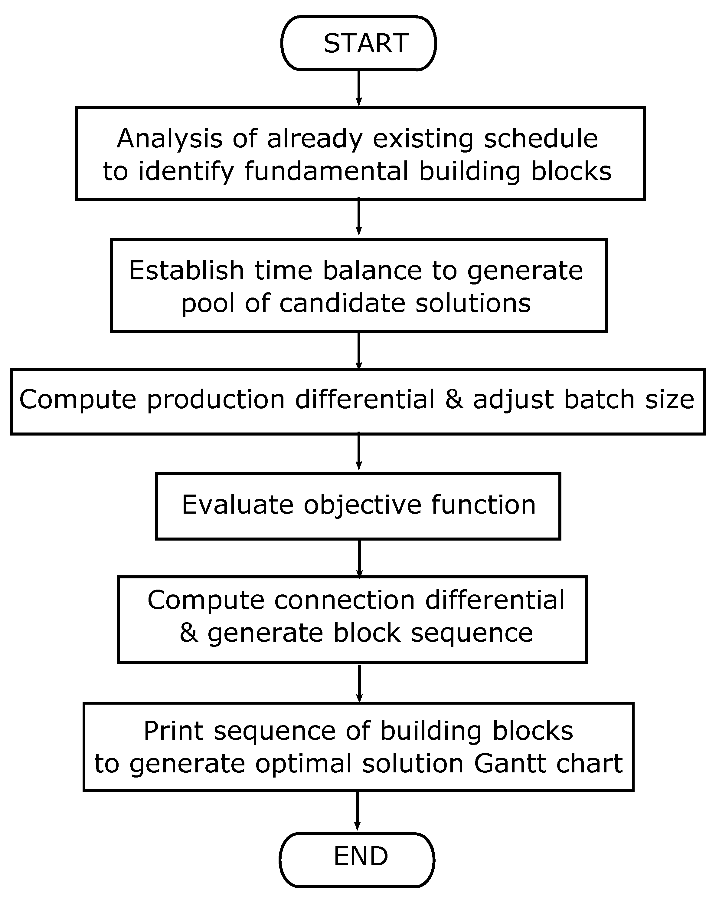
Let us now formulate a framework to construct optimal schedules for energy-integrated batch systems using fundamental building blocks. The corresponding algorithm is depicted in Figure 9. The key steps of the algorithm are discussed below.
Step 1: Identify fundamental building blocks
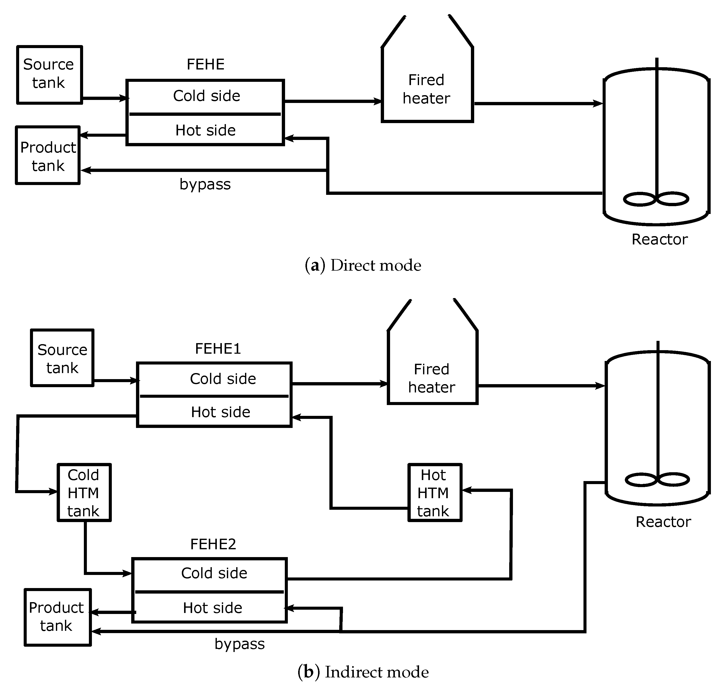
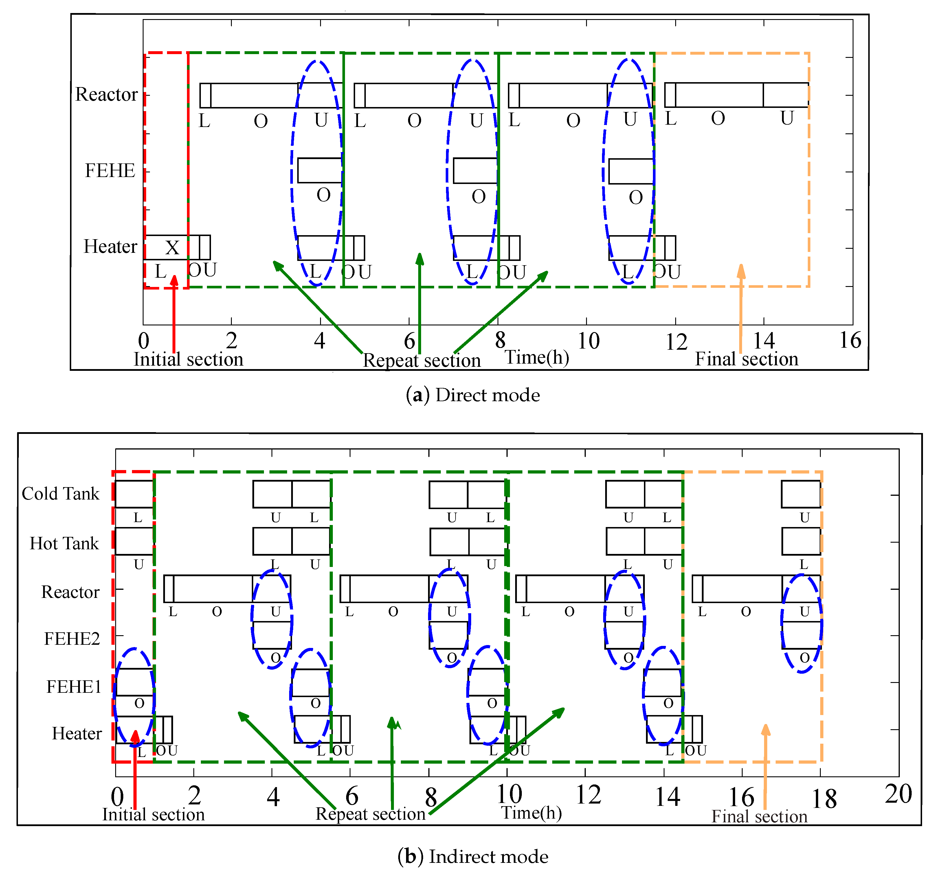
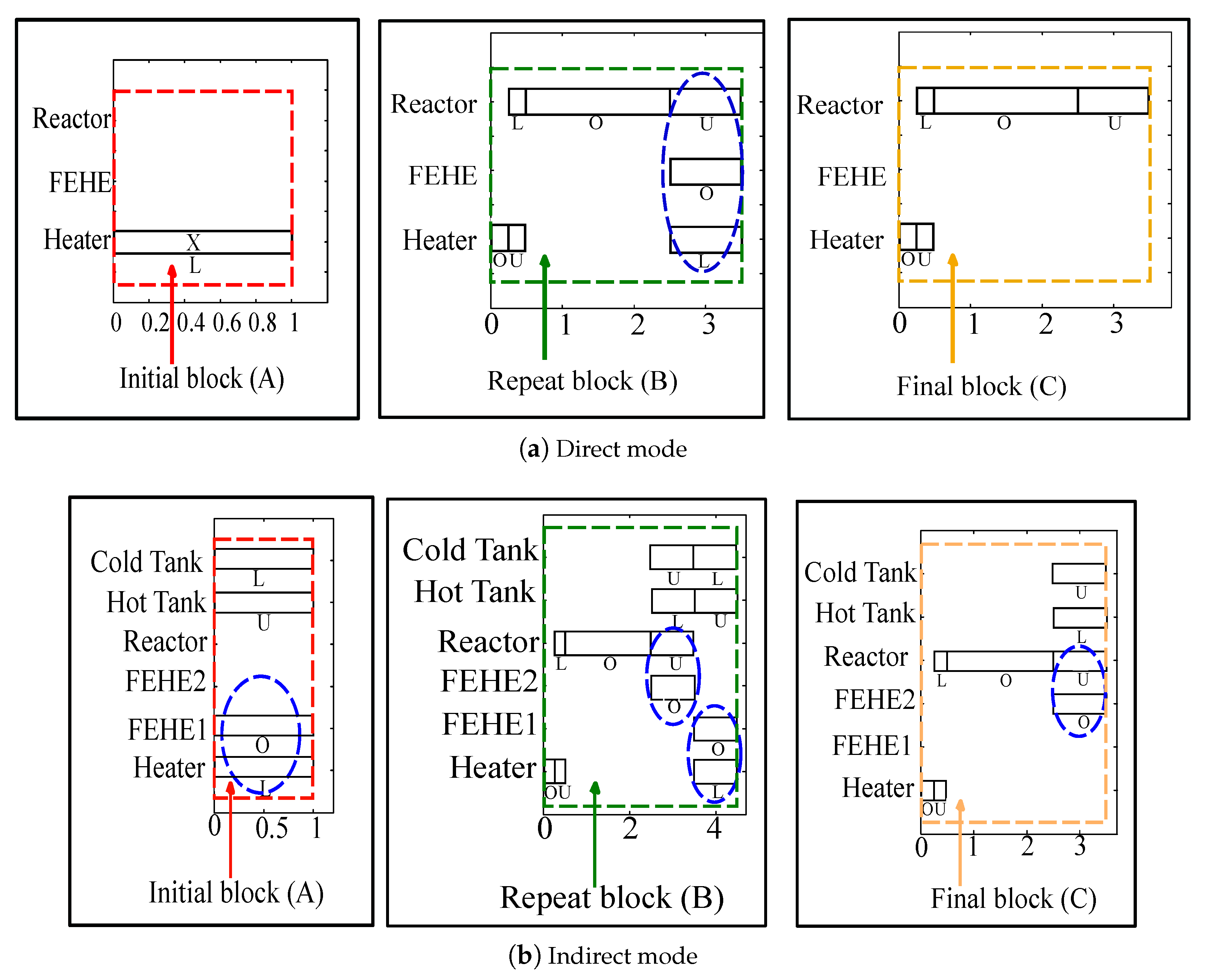
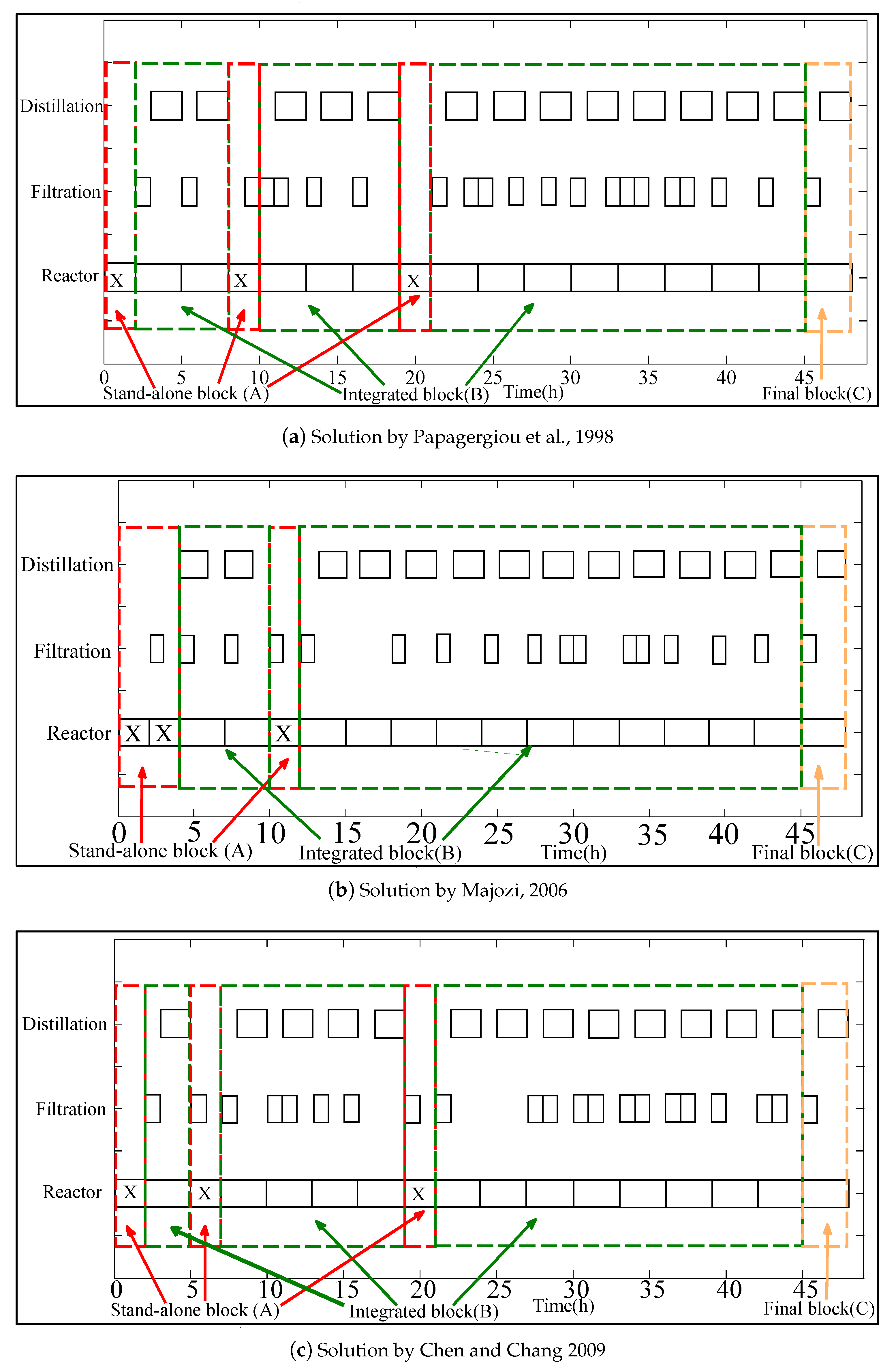
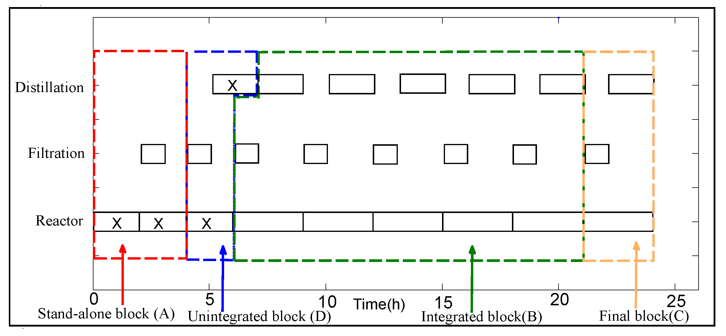
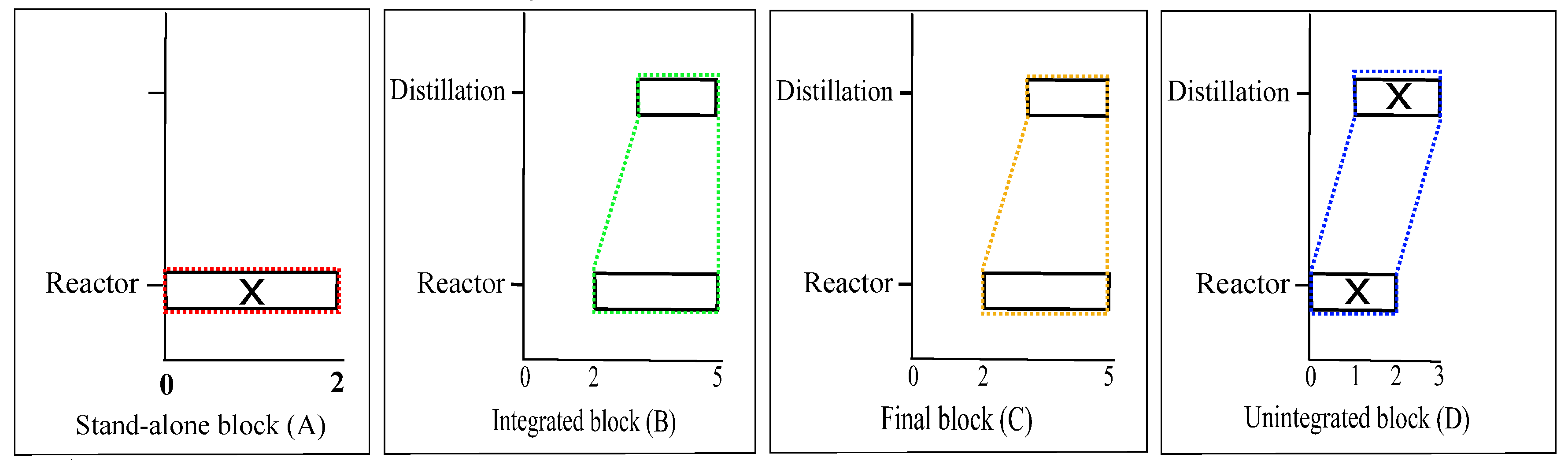
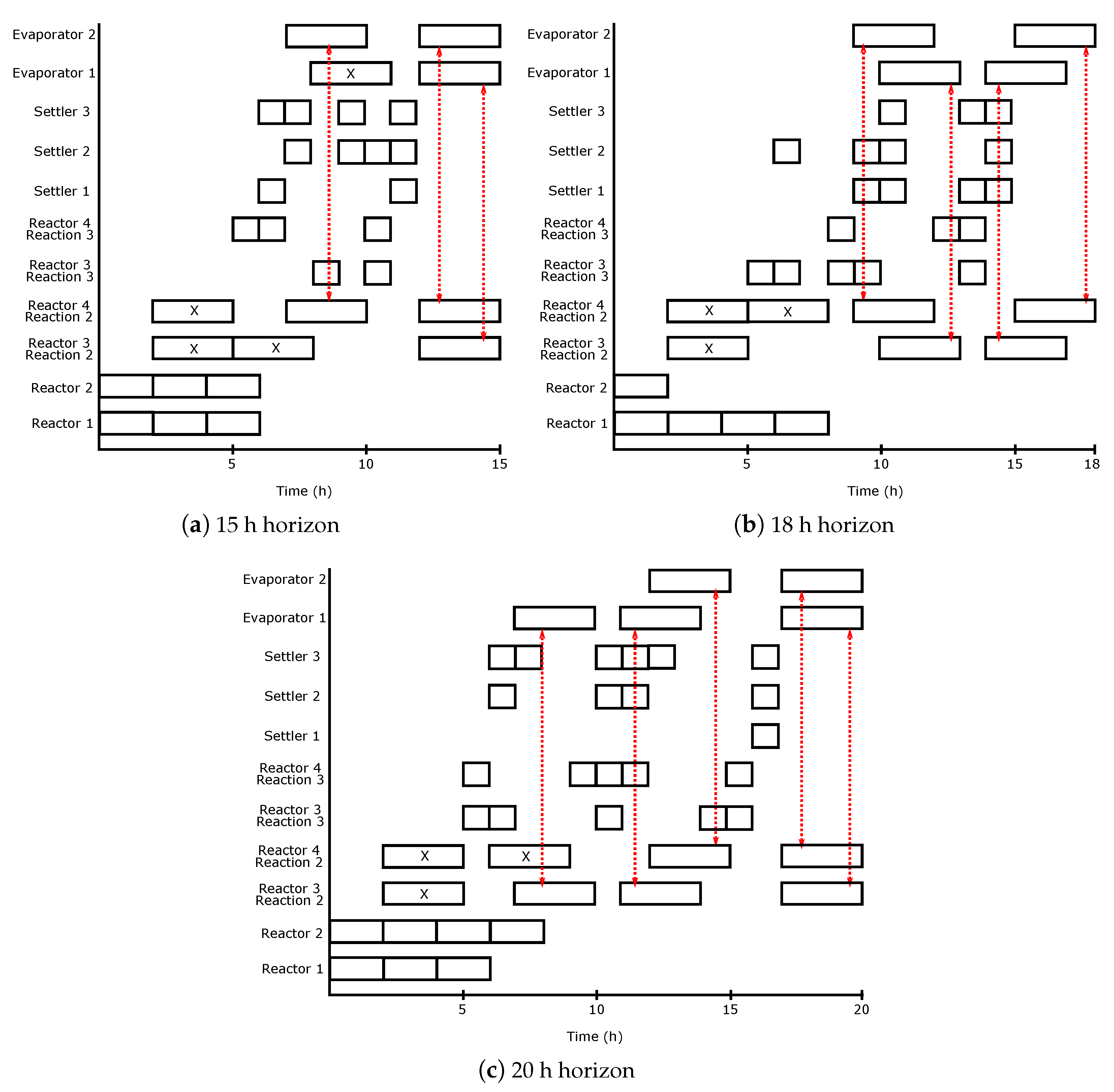
The algorithm starts with the identification of fundamental building blocks present in the optimal solution for any scheduling horizon. Such an optimal solution is obtained by using any of the mixed integer optimization formulations cited in the introduction section. The influence of time-constraints arising from energy integration should be evident in the most frequently appearing building block. For example, in the case of BR-FEHE system with direct integration, the unloading phase of the reactor, the operating phase of the FEHE and the loading phase of the heater will be scheduled at the same time slot and thus would be part of a building block. In the case of BR-S system, Blocks B and C arise due to energy integration time-constraints. Similarly, for the multipurpose industrial example, energy integration between the evaporation task and the Reaction 2 task forces Reactor 3 (or 4) to be scheduled at the same time as Evaporator 1 (or 2), resulting in the repeating patterns shown in Figure 8. In some cases, the physics of the system will decide position and/or location of some of the building blocks. For example, for the BR-FEHE system in direct mode, the initial section acts as a startup phase and is then taken over by the repeat section. On the other hand, for the BR-S system, the final block acts as a closing phase and therefore the optimal schedule will always have one (and only) final block at the end of the scheduling horizon.
Step 2: Establish time balance
Any optimal schedule avoids keeping key/limiting process equipment idle. Naturally, when fundamental building blocks are stitched together to generate the optimal schedule, it is desired that there is minimum idle phase (gap between the building blocks). This is ensured by forcing a time balance constraint and backing off to obtain integer multiplicity for each building block. This can be accomplished by solving the following integer optimization problem:
minimize m i J = T - i = 1 n m i T i subject to J 0 M m i n , i m i M m a x , i
where T is the scheduling horizon, T i is the duration of the ith building block, and M m i n , i and M m a x , i represent the minimum and maximum multiplicity of the ith building block. Depending on the batch system, the above formulation can have multiple solutions and we generate a pool of candidate optimal solutions.
Step 3: Compute production differential and adjust batch size
This step involves meeting the material balance constraints for the intermediate components. Production differential ( Δ ) for an intermediate is defined as the net amount of the intermediate present at the end of the production campaign. It can be computed as the summation of production differential of the individual building blocks ( Δ i , j ) over the scheduling horizon.
Δ = i = 1 n j = 1 m j Δ i , j
where Δ i , j is the net intermediate product produced by the jth instance of the ith block. An optimal schedule requires minimal production differential for all the intermediates. Initially, production differentials are computed for all the candidate solutions obtained in the previous step assuming that all the units/blocks operate at their maximum capacity. Depending on the value of Δ , the following actions are taken to minimize Δ by adjusting capacities of some of the blocks.
  • Δ = 0 : All the processing units are operated at their maximum capacity as it maximizes production while satisfying material balance constraints.
  • Δ < 0 : In this case, the rate of consumption of the intermediate is more than the rate of production. Some of the blocks with net intermediate consumption should therefore be operated at a reduced capacity to satisfy material balance constraints (by increasing Δ to zero). The capacity reduction can be uniform across all the blocks or only few of the blocks can share the capacity reduction. This decision depends on the dependence of the objective function on batch capacity. In case of a linear dependence (or no dependence), both these options result in the same objective function value.
  • Δ > 0 : This is a reverse of the previous case. Production differential in this case can be reduced to zero by operating net intermediate producing blocks at a reduced capacity. As in the previous case, the capacity reduction can be uniform or staggered.
Step 4: Evaluate objective function
Once all the candidate solutions satisfy material balance constraint ( Δ = 0 ), the objective function is evaluated for each of these candidates to select the optimal solution. This step thus fixes the multiplicity of each of the building blocks ( m i ) in the optimal solution.
Step 5: Compute connection differential and generate block sequence
As each of the building blocks can have different intermediate production capacities, the relative position of these blocks affects the dynamic inventory of the intermediate (and determines the intermediate storage requirement). To this end, connection differential ( δ i j ) is defined to capture the net change in the inventory of the intermediate when the ith block is connected with the jth block. As the building blocks are stitched together, the cumulative sum of these connection differentials ( δ c u m ) signifies the corresponding inventory of the intermediate. In order to satisfy dynamic material balance constraint with respect to the intermediate, δ c u m should be non-negative throughout the schedule. The maximum value of δ c u m during the schedule represents the required intermediate storage capacity.
Unlimited or minimum intermediate storage represent two extreme policies considered while solving scheduling problems. The sequence of building blocks can be different for these policies even though the objective function (which typically depends on the number and type of the building blocks) remains the same.
The case of unlimited intermediate storage policy is trivial as it can be accomplished by stacking all the intermediate producing connections ( δ i j 0 ) together before placing the intermediate consuming connections ( δ i j < 0 ). If minimum intermediate storage is desired, each intermediate producing connection should be followed by few intermediate consuming connections without violating material balance constraint ( δ c u m 0 ). This distributes inventory of the intermediate uniformly over the scheduling horizon, thereby minimizing the storage requirement. For example, if δ A , B = 30 , δ B , A = 0 , and δ B , B = - 10 , minimum intermediate storage will be achieved by following a sequence of the form “⋯ABBBBABBBBA⋯” with intermediate storage requirement of 30 units.
The Gantt chart for the optimal solution can now be printed by stitching the building blocks as per the above-obtained sequence.
Remark 1.
The starting point of the proposed method is an optimal solution obtained using rigorous mixed integer optimization. As the entire analysis is pursued with the assumption of optimality of this solution, starting with a non-optimal schedule will severely affect the effectiveness of the method. In such a case, the new schedules obtained by the pattern-based method will also be sub-optimal.
Remark 2.
Identification of the repeating patterns and the corresponding fundamental building blocks in the optimal schedule can be done manually or in automated fashion. For the examples considered in this paper, such blocks are identified manually. One can also automate this process by using graph-based pattern recognition methods available in the published literature [22].
Remark 3.
The proposed method considers two extreme intermediate storage policies in Step 5. One can easily extend these to any other intermediate storage policy. For example, in the case of fixed intermediate storage, instead of distributing intermediate inventory uniformly, one can stack intermediate producing connections ( δ i j 0 ) up to the fixed capacity. This will be followed by few intermediate consuming connections without violating material balance constraint ( δ c u m 0 ).

4. Results and Discussion

Let us now apply this algorithm to the motivating examples presented earlier.

4.1. BR-FEHE System with Direct Integration

Table 1 tabulates details of building blocks for this system. Based on the constraints on the building blocks, it can be noted that the application of the pattern-based algorithm for this system is trivial as there is only one feasible configuration for an optimal schedule. The optimal schedule will always be of the form “AB N C”. The number of B blocks (N) will depend on the scheduling horizon via the time balance in Equation (1). For a scheduling horizon of 50 h, the optimal schedule consists of an A block, followed by 13 B blocks and ends with a C block. If we consider a scheduling horizon of 100 h, the optimal schedule consists of 27 B blocks sandwiched between A and C blocks and results in an idle period of 1 h.

4.2. BR-FEHE System with Indirect Integration

Similar to the direct case, this system also has little flexibility in terms of component arrangement. Building block details for this system are given in Table 2. Any feasible schedule starts with an A block and ends with a C block. In between these, we can have B block(s) or a C–A pair. As a C block uses utility to cool reactor effluent, it needs to be followed by an unintegrated fired heater (A block). This also maintains production differential of zero, so no capacity reduction is required. At this stage, the candidate solutions are of the form “AB N C” or “AB a (CA) ( N - a ) C”. In the next step, objective function is computed for these candidate solutions. Both the candidate solutions produce the same amount of product. However, the utility consumption of the energy-integrated B block is lower than the unintegrated C–A block pair. Thus, optimal solution will always prefer B block over a C–A pair and will be of the form “AB N C”. For a scheduling horizon of 50 h, the optimal schedule consists of an A block, followed by 10 B blocks and ends with a C block (0.5 h of idle time). If we consider a scheduling horizon of 100 h, the optimal schedule consists of 21 B blocks sandwiched between A and C blocks and results in an idle period of 1 h.

4.3. BR-S System

The real utility of the proposed algorithm is evident in this example due to multiplicity of operational alternatives. The corresponding building block details are included in Table 3. For this system, the filter plays a role of shifting inventory of the first intermediate to the second intermediate. As the maximum capacity of the filter is more than the reactor, it can be operated immediately after the reactor with the same production capacity. This eliminates the storage requirement for the first intermediate and we can focus only on the second intermediate.
For this system, any optimal solution starts with an A block and ends with a C block. As shown in Table 3, two of the blocks have a duration of 2 h (A and D), whereas the other two (B and C) have a duration of 3 h. Time balance constraint therefore results in integer solutions of the form (x,y) where x is the total multiplicity of blocks with duration of 2 h and y is the total multiplicity of blocks with duration of 3 h. As every optimal schedule is required to have one C block ( m C = 1 ), the number of B blocks is set as m B = y - 1 . With regards to x, there is a requirement of at least one A block ( m A 1 ), thus all the feasible combinations such that m A + m D = x are considered as candidate solutions. For illustration, let us consider a scheduling horizon of 24 h. The time balance constraint gives integer solutions of the form ( x , y ) = ( 3 , 6 ) , ( 6 , 4 ) , ( 9 , 2 ) . Table 4 tabulates the corresponding candidate solutions.
There are total 18 integer solutions with varying values of production differential Δ . To bring Δ to zero, the following actions are taken.
  • Δ > 0 : Reduce the production capacity of reactor in A or D block as it consumes more cooling water than the reactor in B block. For a large value of Δ , this may reduce the reactor production capacity in these blocks to its minimum processing capacity. In such a case, additionally reduce the production capacity of reactor in B block as required to achieve Δ = 0 .
  • Δ < 0 : Reduce the production capacity of distillation column in D block as it consumes more steam than B or C block. For a large negative value of Δ , this may reduce the distillation production capacity to its minimum processing capacity. In such a case, additionally reduce distillation production capacity in B or C as required to achieve Δ = 0 .
Using these actions, production capacities of individual blocks were updated and the corresponding action is highlighted in Table 4. Based on these updated production capacities, the value of objective function for each of these candidates are computed. As shown in Table 4, the optimal solution consists of two A blocks, five B blocks, one C block and one D block, resulting in the objective value of 1699.84. For this solution, the distillation column in D block is operated at a reduced capacity of 60 T to bring production differential to zero.
These blocks are now stitched together as per the selected intermediate storage policy. The values of various connection differentials for this solution are tabulated in Table 5. For the case of unlimited intermediate storage policy, the optimal sequence is “AADBBBBBC” which results in the maximum intermediate storage requirement of 60 T. Note that this solution is the same as the one obtained by solving mixed-integer optimization formulation (as depicted in Figure 6). For the case of minimum intermediate storage policy, there is only one feasible connection (A–A) with positive connection differential. Therefore, there is no opportunity to distribute inventory of the intermediate across the scheduling horizon and the minimum intermediate storage requirement is the same as the unlimited case. Note that there are multiple feasible sequences, such as “AADBBBBBC”, “AABDBBBBC”, “AABBBDBBC”, etc., which result in the same objective value and storage requirement.
Remark 4.
The pattern-based method allows for optimizing requirement of intermediate storage without incorporating it in the objective function. Unlike mixed-integer optimization formulations where capacity constraint requires specification of intermediate storage capacity, the proposed approach has the ability to minimize intermediate storage based on properties of the patterns. For a scheduling horizon of 48 h, each of the previous methods selects a value of storage capacity. As shown in Table 6, the proposed approach computes maximum (120 T for the case of unlimited storage policy) and minimum (60 T) storage capacity requirements for this scheduling horizon.
Furthermore, this feature of the proposed method can also be used to identify a scheduling horizon which can minimize the intermediate storage requirement. For this BR-S system, a scheduling horizon of 23 h (or any T = 2 + 3 N , N 7 ) does not require any intermediate storage. In the case of mixed-integer optimization, obtaining such a scheduling horizon is challenging and requires a trial and error approach or significant reformulation of the optimization problem.
Remark 5.
The pattern-based approach can also be used to identify time horizons with Δ = 0 . For such horizons, capacity reduction is not required and all the key units operate at their maximum capacity. For this BR-S system, scheduling horizon of 42 h (or any T = 20 N - 18 , N 2 results in Δ = 0 , and thus all the key units are operated at their maximum capacity. This allows maximum utilization of equipment.
Remark 6.
It is well established that mixed-integer optimization formulations do not scale well with an increase in problem size (arising due to the extension of scheduling horizon). However, the pattern-based algorithm scales well with the scheduling horizon. As shown in Table 7, the algorithm scales almost linearly when the scheduling horizon is doubled or even quadrupled. Note that the optimal solution in these cases are quite different and cannot be obtained by simply duplicating solution for a smaller horizon or extending the repeating pattern over a longer horizon as proposed by earlier works [4]. The solution for 24 h case involves unintegrated distillation, whereas, for the case of 48 h, all distillation columns operate in integrated mode.

4.4. Performance Improvement of Mixed-Integer Optimization

The patterns identified for energy-integrated systems can also be used to improve computational performance of mixed-integer optimization. We now demonstrate the effectiveness of a hybrid approach, wherein the solution obtained by the proposed pattern-based method is used to significantly reduce the computational time required for the solution of scheduling formulations. We used continuous time formulation presented by Majozi for demonstration [6]. This formulation consists of material and energy balance constraints, capacity and storage constraints, and sequence and duration constraints. The material and energy balance models were simplified so that the resulting optimization problem had better convergence properties. For example, material balance was expressed in terms of yield and energy balance was expressed in terms of total heating/cooling duty required for the operation.
Continuous time formulations offer significant advantage in terms of reduced number of equations and constraints, however, the optimal performance depends on the correct selection of the required number of time points. The time points refer to the instants on the time-line when any task can start or end, and their total number needs to be specified in the scheduling formulation. Unfortunately, limited literature is available on obtaining the required number of time points to achieve optimal solution. It is quite common to start with a (small) guess value of the number of time points and iteratively increase it till optimal solution is obtained [5]. Each of these iterations requires solving mixed-integer optimization and thus the total computation time grows if the initial guess is far from the required value. Additionally, it is also shown that such a process may result in suboptimal solution [23,24]. Other approaches solve an additional relaxed scheduling problem to obtain the optimal number of time points [23,24]. As the proposed pattern-based method generates a feasible schedule, the number of required time points can be directly counted from this solution. Figure 10 shows a parity plot for the predicted and actual number of time points required to solve the BR-S problem for various scheduling horizons. It can be seen that the pattern-based method is able to correctly predict the minimum number of time points required to initialize continuous time formulation, thereby reducing the required computational effort.
Furthermore, the solution obtained by the pattern-based method can also be used to simplify the scheduling formulation. For example, if the optimal solution by the pattern-based method results in Δ = 0 , the equipment capacity constraints can be neglected in the scheduling formulation as all the units operate at their maximum capacity. For the BR-S system, if Δ < 0 , the reactor always operates at its maximum capacity and the distillation operates only in integrated mode. We therefore used the pattern-based algorithm to compute Δ and simplified the scheduling formulation of Majozi in terms of the production capacity constraints and permissible modes of operation. Table 8 tabulates the comparison between stand-alone mixed-integer optimization and the hybrid approach. All optimizations were performed using GAMS/SCIP (General Algebraic Modeling System/Solving Constraint Integer Programs) solver on a 3.2 GHz Pentium i7 processor. It is encouraging to note that the hybrid approach is able to reduce the computational effort by orders of magnitude while maintaining optimality of the solution.

5. Conclusions

In the context of online rescheduling as a policy to reject operational disturbances, there is a need to repeatedly generate optimal schedules via computationally efficient methods. To this end, we present a pattern-based method to generate schedules for energy-integrated batch process systems. The framework is based on the observation that time-constraints in energy integration give rise to specific repeating patterns in the optimal schedules. Furthermore, it is shown that these optimal schedules consist of combinations of few building blocks. A pattern-based scheduling algorithm is therefore developed to obtain the number and optimal sequence of these building blocks, and thus allows for constructing optimal schedule for any scheduling horizon.
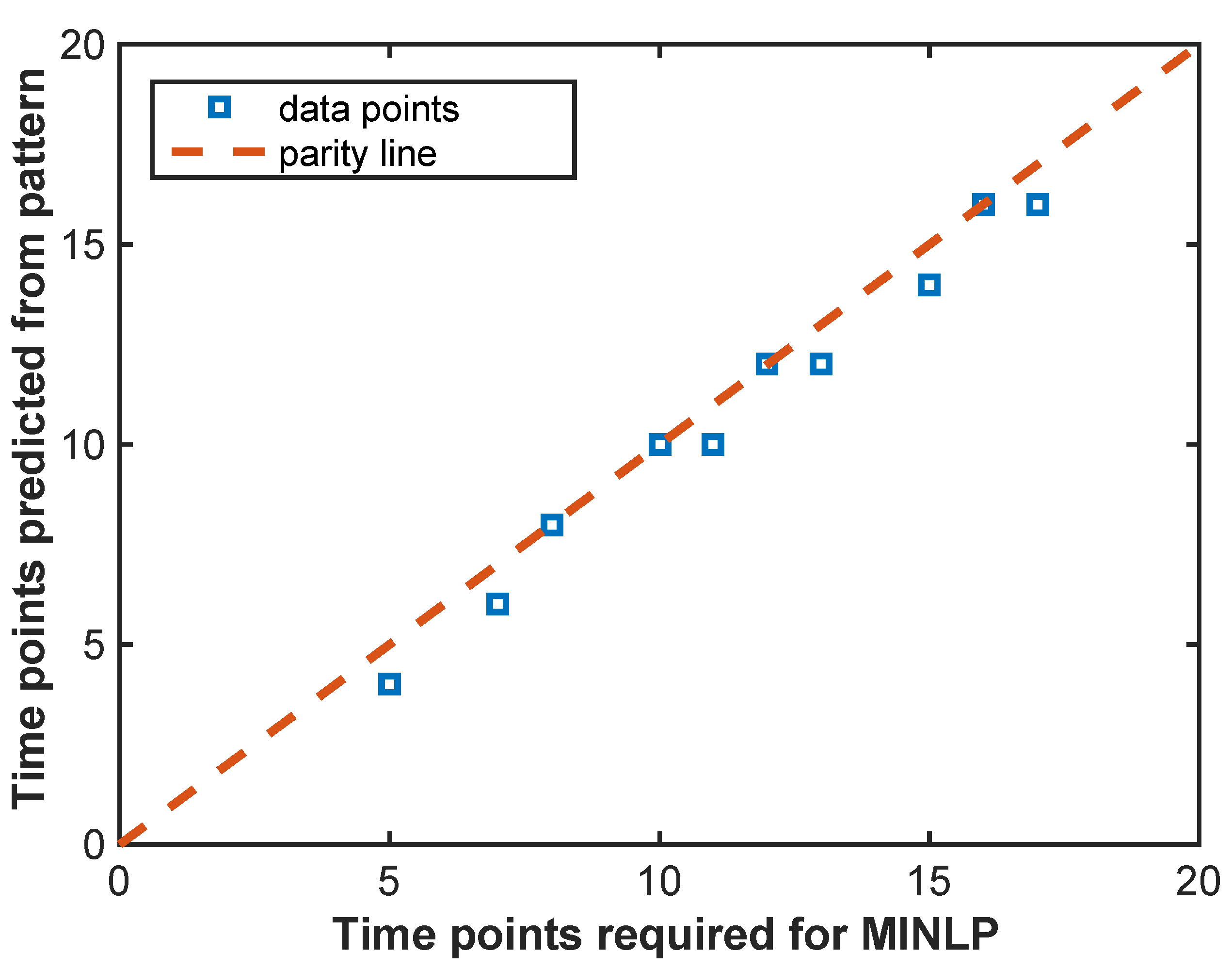
With the help of a benchmark example system of a reactor and a distillation column, it is shown that the proposed method is able to generate optimal schedules which match solution of rigorous mixed-integer optimization and requires significantly less computation time. The method is scalable to larger scheduling horizons and helps identify scheduling horizons which can reduce intermediate storage or maximize utilization of equipment. Furthermore, the method can also be coupled with mixed-integer optimization to significantly reduce the computation time of the latter through prediction of the required number of time points and simplification of the scheduling formulation. Thus, the proposed method is a suitable candidate for application in online rescheduling.
The proposed method is developed for profit maximization in the case of a single product train with fixed duration. In principle, it can also be developed for the case of batch size-dependent duration, makespan minimization or more complex arrangements such as multi-product or multi-purpose schemes. Our ongoing research is exploring such extensions.

Author Contributions

The concept development is done by S.S.J. The method is developed by S.M. and S.S.J. Implementation, results and validation is done by S.M. and S.S.J. Original draft is written by S.M. Review and Editing is done by S.S.J. Funding Acquisition is done by S.S.J and C.S.M.

Funding

This research was funded by the Government of India, Department of Science and Technology (DST) grant numbers INSPIRE (IFA 13 ENG 61) and SERB-SB/S3/CE/090/2013.

Conflicts of Interest

The authors declare no conflict of interest. The funders had no role in the design of the study; in the collection, analyses, or interpretation of data; in the writing of the manuscript, or in the decision to publish the results.

Abbreviations

The following abbreviations are used in this manuscript:
BR-FEHEBatch reactor-feed effluent heat exchanger
HTMHeat transfer medium

References

  1. Fernández, I.; Renedo, C.J.; Pérez, S.F.; Ortiz, A.; Mañana, M. A review: Energy recovery in batch processes. Renew. Sust. Energy Rev. 2012, 16, 2260–2277. [Google Scholar] [CrossRef]
  2. Papageorgiou, L.G.; Shah, N.; Pantelides, C.C. Optimal scheduling of heat integrated multipurpose plants. Ind. Eng. Chem. Res. 1994, 33, 3168–3186. [Google Scholar] [CrossRef]
  3. Kondili, E.; Pantelides, C.C.; Sargent, R.W.H. A general algorithm for short-term scheduling of batch operations—I. MILP formulation. Comput. Chem. Eng. 1993, 17, 211–227. [Google Scholar] [CrossRef]
  4. Lee, B.; Reklaitis, G.V. Optimal scheduling of cyclic batch processes for heat integration—I. Basic formulation. Comput. Chem. Eng. 1995, 19, 883–905. [Google Scholar] [CrossRef]
  5. Ierapetritou, M.G.; Floudas, C.A. Effective continuous-time formulation for short-term scheduling. 1. Multipurpose batch processes. Ind. Eng. Chem. Res. 1998, 37, 4341–4359. [Google Scholar] [CrossRef]
  6. Majozi, T. Heat integration of multipurpose batch plants using a continuous-time framework. Appl. Therm. Eng. 2006, 26, 1369–1377. [Google Scholar] [CrossRef]
  7. Holczinger, T.; Hegyháti, M.; Friedler, F. Simultaneous heat integration and batch process scheduling. Chem. Eng. Trans. 2012, 29, 337–342. [Google Scholar]
  8. Adonyi, R.; Romero, J.; Puigjaner, L.; Friedler, F. Incorporating heat integration in batch process scheduling. Appl. Therm. Eng. 2003, 23, 1743–1762. [Google Scholar] [CrossRef]
  9. Chen, C.L.; Ciou, Y.J. Design and optimization of indirect energy storage systems for batch process plants. Ind. Eng. Chem. Res. 2008, 47, 4817–4829. [Google Scholar] [CrossRef]
  10. Castro, P.M.; Barbosa-Póvoa, A.P.; Matos, H.A. Optimal periodic scheduling of batch plants using RTN-based discrete and continuous-time formulations: a case study approach. Ind. Eng. Chem. Res. 2003, 42, 3346–3360. [Google Scholar] [CrossRef]
  11. Halim, I.; Srinivasan, R. Sequential methodology for scheduling of heat-integrated batch plants. Ind. Eng. Chem. Res. 2009, 48, 8551–8565. [Google Scholar] [CrossRef]
  12. Powell, K.M.; Cole, W.J.; Ekarika, U.F.; Edgar, T.F. Optimal chiller loading in a district cooling system with thermal energy storage. Energy 2013, 50, 445–453. [Google Scholar] [CrossRef]
  13. Powell, K.M.; Kim, J.S.; Cole, W.J.; Kapoor, K.; Mojica, J.L.; Hedengren, J.D.; Edgar, T.F. Thermal energy storage to minimize cost and improve efficiency of a polygeneration district energy system in a real-time electricity market. Energy 2016, 113, 52–63. [Google Scholar] [CrossRef]
  14. Westberg, B.; Machalek, D.; Denton, S.; Sellers, D.; Powell, K. Proactive Automation of a Batch Manufacturer in a Smart Grid Environment. Smart Sustain. Man Syst. 2018, 2, 110–131. [Google Scholar] [CrossRef]
  15. Roslöf, J.; Harjunkoski, I.; Björkqvist, J.; Karlsson, S.; Westerlund, T. An MILP-based reordering algorithm for complex industrial scheduling and rescheduling. Comput. Chem. Eng. 2001, 25, 821–828. [Google Scholar] [CrossRef]
  16. Méndez, C.A.; Cerdá, J. Dynamic scheduling in multiproduct batch plants. Comput. Chem. Eng. 2003, 27, 1247–1259. [Google Scholar] [CrossRef]
  17. Zhao, X.G.; O’neill, B.K.; Roach, J.R.; Wood, R.M. Heat integration for batch processes: part 1: Process scheduling based on cascade analysis. Chem. Eng. Res. Des. 1998, 76, 685–699. [Google Scholar] [CrossRef]
  18. Mete, S.; Jogwar, S.S. A Pattern-based Method for Scheduling of Energy-integrated Batch Process Networks. IFAC-PapersOnLine 2016, 49, 669–674. [Google Scholar] [CrossRef]
  19. Jogwar, S.S.; Daoutidis, P. Dynamic characteristics of energy-integrated batch process systems: Insights from two case studies. Ind. Eng. Chem. Res. 2015, 54, 4326–4336. [Google Scholar] [CrossRef]
  20. Chen, C.L.; Ciou, Y.J. Design of indirect heat recovery systems with variable-temperature storage for batch plants. Ind. Eng. Chem. Res. 2009, 48, 4375–4387. [Google Scholar] [CrossRef]
  21. Majozi, T.; Zhu, X.X. A novel continuous-time MILP formulation for multipurpose batch plants. 1. Short-term scheduling. Ind. Eng. Chem. Res. 2001, 40, 5935–5949. [Google Scholar] [CrossRef]
  22. Conte, D.; Foggia, P.; Sansone, C.; Vento, M. Thirty years of graph matching in pattern recognition. Int. J. Pattern Recognit. 2004, 18, 265–298. [Google Scholar] [CrossRef]
  23. Li, J.; Floudas, C.A. Optimal event point determination for short-term scheduling of multipurpose batch plants via unit-specific event-based continuous-time approaches. Ind. Eng. Chem. Res. 2010, 49, 7446–7469. [Google Scholar] [CrossRef]
  24. Seid, R.; Majozi, T. A novel technique for prediction of time points for scheduling of multipurpose batch plants. Chem. Eng. Sci. 2012, 68, 54–71. [Google Scholar] [CrossRef]
Figure 1. Energy-integrated Batch Reactor-Feed Effluent Heat Exchanger (BR-FEHE) system (HTM: Heat transfer medium).
Processes 07 00103 g001
Figure 2. Optimal schedules for the BR-FEHE system (L, loading phase; U, unloading phase; O, operating phase; X, stand-alone mode).
Processes 07 00103 g002
Figure 3. Fundamental building blocks for optimal schedule of BR-FEHE system.
Processes 07 00103 g003
Figure 4. Heat-integrated batch reactor-separator (BR-S) system.
Processes 07 00103 g004
Figure 5. Optimal schedules for BR-S system (X, stand-alone mode).
Processes 07 00103 g005
Figure 6. Optimal schedule for BR-S system for 24 h horizon.
Processes 07 00103 g006
Figure 7. Fundamental building blocks for optimal schedule of BR-S system.
Processes 07 00103 g007
Figure 8. Optimal schedule for multipurpose industrial example(←→ represents energy integration).
Processes 07 00103 g008
Figure 9. Pattern-based scheduling algorithm.
Processes 07 00103 g009
Figure 10. Prediction of required number of time points.
Processes 07 00103 g010
Table 1. Component details for Batch Reactor-Feed Effluent Heat Exchanger (BR-FEHE) system with direct integration.
Block Δ T (h)Constraints
A01.251 unit required at the start of the schedule
B03.5cannot be the first unit of the schedule
C03.251 unit required at the end of the schedule
Table 2. Component details for BR-FEHE system with indirect integration.
Block Δ T (h)Constraints
A−1 hot (+1 cold)11 unit required at the start of the schedule
B04.5cannot be the first unit of the schedule
C+1 hot (−1 cold)3.51 unit required at the end of the schedule
Table 3. Component details for Batch Reactor-Separator (BR-S) system.
Block Δ T (h)Constraints
A+6021 unit required at the start of the schedule
B−103cannot be the first unit of the schedule
C−7031 unit required at the end of the schedule
D−102cannot be the first unit of the schedule
Table 4. Candidate solutions for BR-S system for scheduling horizon of 24 h (optimal solution highlighted in bold).
SN m A m B m C m D Δ (T)Capacity ReductionJ (rcu)
1351060Reactor (A)1549.44
22511−10Distillation (D)1699.84
31512−80Distillation (D)1682.24
46310260Reactor (A)969.68
55311190Reactor (A)1148.08
64312120Reactor (A)1326.48
7331350Reactor (A)1504.88
82314−20Distillation (D)1627.28
91315−90Distillation (D)1609.68
109110460Reactor (A,B)356.72
118111390Reactor (A,D)568
127112320Reactor (A,D)746.72
136113250Reactor (A)925.12
145114180Reactor (A)1103.52
154115110Reactor (A)1281.92
16311640Reactor (A)1460.32
172117−30Distillation (D)1554.72
181118−90Distillation (D)1537.12
Table 5. Connection differentials for 24 h scheduling horizon solution of BR-S system.
Connection δ (T)Connection δ (T)Connection δ (T)
A–A60B–A60D–A60
A–B−10B–B−10D–B−10
A–C−10B–C−10D–C−10
A–D0B–D0
Table 6. Comparison of optimal solutions for 48 h scheduling horizon solution for BR-S system.
ApproachObjective Value (rcu)Storage Requirement (T)
Papageorgiou et al.3644.690
Majozi3644.6110
Chen and Chang3644.680
Present work—Unlimited storage policy3644.6120
Present work—Minimum storage policy3644.660
Table 7. Solution statistics for BR-S system for different scheduling horizons.
T (h)J (rcu)CPU Time (s)Characteristic Feature
241699.81.69un-integrated distillation
483644.62.10reduced capacity integrated distillation
967507.33.75un-integrated distillation
Table 8. Performance comparison for BR-S system.
T (h) Δ (T)ApproachObjective Value (rcu)CPU Time (s)
20−60MINLP1361.301568
Hybrid1361.302.56
2170MINLP1457.001680
Hybrid1457.004.88
220MINLP1562.202216
Hybrid1562.206.94

