1. Introduction
There are several industrial processes that require heat from 60–250 °C [
1], where this heat can be provided with solar thermal systems. There are different suitable technologies according to the temperature range; low-temperature collectors, up to 90 °C (flat plate collectors, evacuated tube collectors, etc.) and medium temperature collectors up to 250 °C (compound parabolic collectors, linear Fresnel, parabolic trough, etc.). The main challenge to achieve the implementation of these systems into industrial processes is the variation of heat requirements, temperature ranges, and type of processes with each industrial case. Several studies focus on integrating solar thermal systems into industrial processes. One of the most detailed works was developed by the International Energy Agency, within the Solar heating and cooling program, in the framework of Task 49 “Solar heat integration in industrial processes” [
2,
3], where methodologies and a detailed guide are presented to perform the integration of solar heat in industrial or commercial processes. In addition, Farjana et al. [
4] reported a global review about the potential application of solar technologies to industrial processes and sectors where solar heat is currently used, as well as the solar technologies available, the heat demand of industries and their temperature ranges. Among their main findings is the current limitation to insert solar heating technologies directly into the processes, which is related to the high initial investment costs. These problems are considered a barrier to implement these types of projects to small and medium companies. The authors recommend carrying out numerical simulations to analyze the efficiency and temperature that can be obtained with solar technologies integrated to the industrial processes along different periods, and in addition, to perform a cost analysis and determine the payback time. Finally, it is advised to carry out a life cycle analysis to demonstrate the reduction in the emission of greenhouse gases to calculate the long-term impact.
Modeling and simulation are essential tools for the integration of solar thermal systems into industrial processes, since they allow predicting the performance of each integrated system [
5]. Furthermore, the sizing of components within a system based on renewable energies is a complex problem. Moreover, managing different configurations is needed to select the most appropriate one for each particular application, without the need to invest many resources, both economic and time. For this reason, computational modeling presents several advantages, including the exclusion of prototypes costs, the analysis in the organization of complex systems, the probability of optimizing the components, the possibility of estimating the energy flows of the system, among others [
6].
In the literature, models have been developed describing the performance of solar thermal systems using different software and validating with experimental data. [
7,
8,
9,
10]. Research has been done on the potential, integration, and monitoring of solar thermal plants [
11,
12,
13,
14,
15,
16].
Models have also been developed in TRNSYS (Transient System Simulation Tool), which is a complex modular simulation software that allows the dynamic simulation of energy systems, and hence is mainly used to simulate installations containing systems which work with renewable energies, including solar thermal [
5,
17,
18,
19]. The accuracy of the results obtained using TRNSYS is high and predicts the performance of solar thermal systems adequately; nevertheless, it is a commercially licensed software and requires considerable training to use it. For this reason, instead of using TRNSYS, several authors have developed alternative simulation tools using spreadsheets or programs in languages such as C/C++, JAVA, etc. [
5].
Among these cases is Karagiorgas et al. [
20], who presented a tool for the use of heat pumps and solar air collectors applied to the air conditioning of the National Center for Renewable Energy Sources of Greece. The results obtained with the proposed tool were compared with those of TRNSYS for validation; the energy consumption, the seasonal solar radiation, and the solar heat production were higher by 3.04%, 5.81%, and 12.90%, respectively, while the solar fraction was sub estimated by 8.74%. Bunea et al. [
21] developed a model using Polysun to simulate the performance of a solar heat generation system installed in the company “COLAS”, based on high vacuum solar collectors working with temperatures of up to 200 °C. The first results were 2.6 times lower than the initial estimates and the model has yet to be validated. Kulkarni et al. [
22] proposed a methodology to determine the “design space” of solar water heating systems. Design space consists of analyzing collector area vs. storage volume diagrams with constant solar fraction lines; with this, a multi-objective optimization was performed to minimize the annual life cycle cost of solar water heating systems. Picón-Nuñez et al. [
23], developed a tool for designing and selecting the most appropriate network array for a given application using the values of specific drop pressure, temperature, and heat requirement as functions. They presented a thermo-hydraulic model for solar collector networks and their solution was shown graphically using the length of the exchanger against the number of arrays in parallel.
All these works focus on the analysis of thermal performance in particular processes and do not consider the installation and operation costs associated with the array of solar collectors.
In other approaches, the work carried out by Bava et al. [
24] showed through TRNSYS simulations that the annual useful energy transferred to the heat exchanger was 1.2% higher than the values measured experimentally, but the seasonal basis deviations were +7% and −8%, for the June–December 2013 and January–May 2014 periods, respectively. Almeida et al. [
25] compared the performance of an energy system using TRNSYS over periods longer than one month, and it was found that the differences with respect to the experimental results were less than 3%.
There are complex works that consider economic analysis, such as Silva et al. [
26], who carried out the thermo-economic optimization of a parabolic trough solar plant for industrial processes using memetic algorithms; the variables considered in the optimization routine were the number of collectors in series, the number of rows, the space between rows, and the storage volume.
Accordingly, this work describes a computational tool based in a commercial spreadsheet. It allows simulating through a parametric analysis, the performance of a field of solar collectors in different series–parallel arrays. It calculates the temperature on the fluid inside the storage tank, the useful heat from the collector field, the heat required by the process, and the auxiliary energy needed. This tool was validated with experimental data and compared with results obtained using TRNSYS. Additionally, this work proposes a methodology to determine the number of collectors and the optimal series-parallel arrays, taking into account the cost of pipeline and pumping, which is currently complicated to evaluate using TRNSYS.
2. Theoretical Model
The determination of the technical-economic feasibility of a solar heating system depends mainly on knowing the solar fraction, which is the ratio between the solar contribution to the load and the total load [
27] (pp. 665–686). Simulation tools are commonly used for this purpose.
Figure 1 shows the considered system for the sizing of a low temperature solar thermal system. This system includes a solar collector array, a storage tank, and a heat exchanger.
Tmu is a constant mass flow rate of water with constant temperature. The heat exchanger stands for the operation with different fluids and pressures, as in applications for space heating or other applications where the climate conditions reach freezing temperatures.
The analysis developed was divided into three main parts: the storage tank, the solar collector field, and the techno-economic analysis.
2.1. Storage Tank
In order to analyze the storage tank, the following assumptions were made: water is pressurized and perfectly mixed; the heat exchanger, along with the connecting pipes between the solar array, the storage tank, and the heat exchanger, are completely insulated, so there are no thermal losses to the surrounding. Finally, the specific heat of collector, load, and storage tank fluids, Cpc, CpL and Cps, are constant in all ranges of operation temperature.
The equation that describes the energy balance in the storage tank is given by [
28] (pp. 426–444):
where
is the useful heat gain by the solar collectors (the sign + indicates that only positive values are taken into account), second and third terms on the right correspond to the heat transfer within the heat exchanger and the ambient heat losses in the storage tank, respectively.
Using the Euler simple integration method to discretize the Equation (1) in the time interval Δ
t, the temperature variation of the water in the storage tank is obtained:
where
is the temperature of the next state? It is important to consider using a sufficiently small time interval to ensure the stability of the integration scheme [
28] (pp. 426–444).
2.2. Solar Collector Field
On the other hand, the thermal performance of a collector field not only depends on the individual efficiency of each collector, but it also depends on how these are interconnected. In the thermal analysis, a collector connected in series must consider interconnection heat losses. The useful heat of two or more solar collectors connected in series is determined by the energy gain in each collector along to the heat losses in the interconnection pipes [
29], as shown in
Figure 2. As a result, the temperature at the outlet of the first collector,
, is greater than the temperature at the entrance of the second collector,
, due to the heat losses,
, of the interconnection pipe.
Duffie and Beckman [
28] (pp. 426–444) explain the procedure to develop a simplified equation to obtain the useful heat of
N identical collectors connected in series:
where
and
are respectively, modified optical efficiency and modified collector overall heat loss coefficient, taking into account the heat losses in the pipelines, and
is the removal factor that considers the presence of a heat exchanger [
28] (pp. 426–444).
Finally,
is defined by:
Solar Radiation
In the sizing of a low-temperature solar thermal system (up to 150 °C), it is necessary to know the total incident radiation over the collector’s surface according to their slope. This can be obtained from known data of horizontal radiation (global or beam) on the study site according to its geographical position. There are several mathematical models to perform this estimation of the beam and the diffuse radiation on a tilted surface. This methodology uses the mathematical model described by Pérez et al. [
30,
31], which uses beam, global, or diffuse radiation data on a horizontal surface, considering an anisotropic sky; that is a sky that takes into account the circumsolar diffuse and the horizon contributions, in addition to the diffuse isotropic dome of the sky.
2.3. Techno-Economic Analysis
An economic analysis based on the payback time was incorporated into the computing tool, and the annual costs of the whole system and the savings of the solar thermal system are taken into account. Solar savings over a year are given by:
The unpaid balance of the investment in the solar thermal system is given by:
For the annual payback time,
, the following functions are considered:
The function of Equation (7) allows identifying when the unpaid balance passes from a negative to a positive value and adding one by one the years when it is still negative. Equation (8) allows determining the fractional value of the payback time if the current value
is different from the previous value. Adding Equations (7) and (8), the payback time
is obtained, in years:
4. Results and Discussions
The developed model requires the geographical position of the site, solar irradiation, and meteorological data (ambient temperature and wind speed) generated hourly from a typical meteorological year (TMY), the temperature of the water supply, the temperature required by the process, the slope of the collectors, and the profile of the thermal load. The volume of the thermal storage tank was defined with the daily volume of hot water required. The heat exchanger effectiveness was set up with a value similar to a compact type, that corresponds to a heat capacity rate ratio up to 0.5 and NTU of 2–4 [
32] (pp. 48–52), and the overall heat loss coefficient of the hot water tank corresponds to the value experimentally calculated and reported by Venegas-Reyes [
33], whose data was used to perform the model validation.
Table 1 shows the parameters used in the simulations for a hypothetical process in the city of Delicias, Chihuahua, which consists in providing hot water at 90 °C to an absorption cooling system.
Additionally,
Table 2 shows the parameters of the evacuated heat pipe collector whose operating range is within the temperature required by the process. The collector slope was established as the value of location latitude, and the gross area, the mass flow rate, the optical efficiency, and the overall heat loss coefficient were taken from the solar collector evaluation certificate, according to the SRCC Standard 100-2008-02 [
34].
The coefficients of the polynomial regression were obtained from data of transverse incidence angle modifier
:
While
Table 3 shows the data used for the economic analysis.
4.1. Model Validation
The model was validated based on the data reported in Venegas-Reyes [
33], where five collectors were connected in series and coupled to a storage tank of 120 L. The system was pressurized to avoid water’s phase change. The test was performed circulating water from the storage tank to the collectors and returning it to the tank, accumulating the heat. In this way, it was possible to increase the water temperature from an initial value of 58.4 °C to a final value of 132.9 °C.
Figure 4 shows the water temperature in the storage tank for both experimental data and model. The experimental values of temperature and the values obtained with the model show an average relative error of 2.16%.
4.2. TRNSYS Comparison
Additionally, a comparison of the model using TRNSYS was carried out, considering that heat losses in the connection pipes of each solar collector were not taken into account in the simulations. Using the data from
Table 1 and
Table 2, the system in
Figure 1 was simulated, both in the proposed computational tool and with TRNSYS. The main objective of this comparison was to verify that the solar fraction (over a year of operation) estimated with both, the model and TRNSYS, were equal.
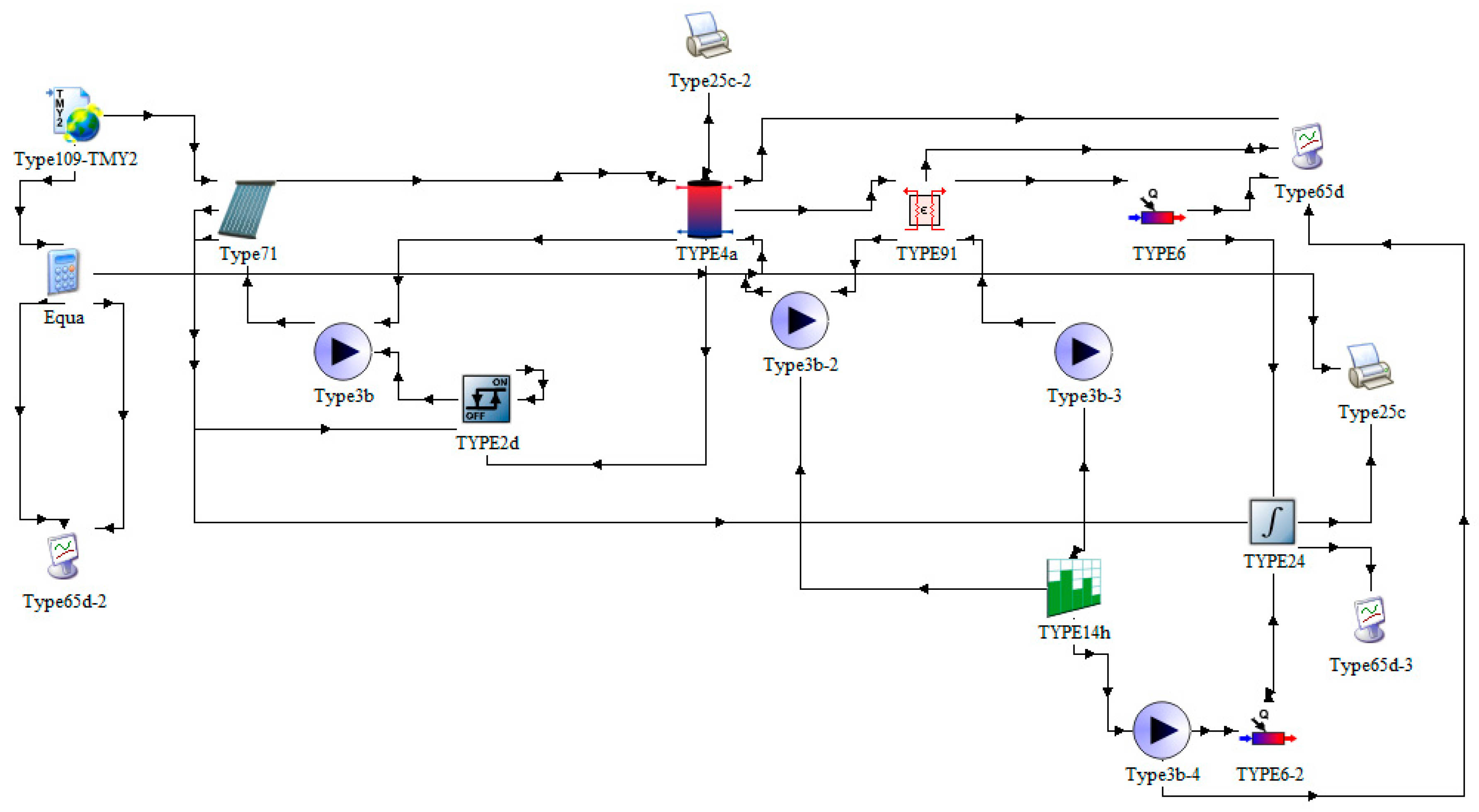
The system in
Figure 1 was implemented in a TRNSYS workspace, as shown in
Figure 5. The collector field (Type 71) is connected to the storage tank modeled with the Type 4a, this is a stratified tank where a single node is being considered to emulate a fully mixed tank, this is connected to the heat exchanger (Type 91) in the load side, with a known effectiveness (e.g., of a technical sheet). There are four pumps: the Type3b pump supplies water to the collectors and to the hot side of the storage tank. The Type3b-2 pumps the fluid from the storage tank to the heat exchanger, Type3b-3 pumps the make-up fluid from the thermal load. An auxiliary heater (Type 6) and a Type3b-4 pump with a Type6-2 heater emulate a conventional heating system.
Figure 6 shows the temperature profiles of the water in the storage tank, calculated with the proposed tool (Equation (2)) and with the TRNSYS model, every hour of the period from 31 January (hours 1–24) to 1 February (hours 25–48). It is observed that the thermal performance of the tank calculated with the proposed tool is sensitive to solar radiation. During the first hour of heat extraction to the process (from 7–8 h, and from 31–32 h), it presents a temperature decrease of 9 °C, and this is due to the fact that heat is extracted when the minimum solar radiation value required to gain heat from the solar collectors has not yet been reached. Similar behavior occurs when the heat extraction ends (17 h, and 41 h), since there is no solar radiation available, the temperature decreases dramatically during the following hour, around 8 °C. In contrast, the results obtained with the TRNSYS model are more stable, because the pumping to the tank is being controlled with regard to the critical level of radiation. As for the period between 18 h and 31 h, when there is no solar radiation, the behavior calculated with both tools is quite similar.
Taking as a reference the temperature profile of the water inside the thermal storage tank obtained with TRNSYS throughout the typical meteorological year, and comparing it with the temperature profile of the storage tank water from the developed tool, the relative error and the standard deviation of this error was calculated for different sizes of collector fields:
Figure 7 shows the standard deviation of the relative error between the proposed tool and TRNSYS as a function of the collector area, where the highest value was 6%.
Although the proposed tool shows a more unstable response at the beginning and the end of the simulation, also, at the beginning and the end of solar radiation availability, when doing the analysis over a year of operation, the solar fraction values result very similar to those obtained with the simulation in TRNSYS.
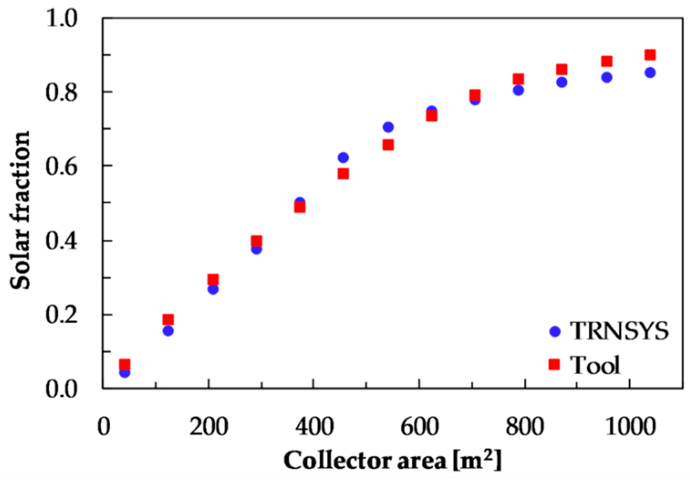
Figure 8 presents the solar fractions obtained with the proposed tool and with the TRNSYS model. It is observed that results are quite similar, with a standard deviation of the relative error of 6.8%.
In a first approximation, it was considered that collectors are all connected in parallel, which, from a thermal analysis, is optimal since the thermal losses are less, however, this is not necessarily optimal in a technical-economic perspective.
Figure 9 shows the solar fraction and payback time according to the collector’s area, considering as a first approximation, the cost of collector area, storage tank, and a percentage of both as installation cost. Throughout a parametric analysis, which consists of increasing the number of collectors in parallel on each iteration, it was determined from a thermal analysis that the optimal area of solar collection is 665.3 m
2. That area corresponds to 160 collectors connected in parallel and results in a payback time of 7.43 years and a solar fraction of 0.772.
Once the optimal collector area was determined with the thermal analysis, the technical-economic optimization was carried out for the different series-parallel arrays. The costs of solar collectors, thermal storage, piping, and pumping power were taken into account.
Figure 10 shows a schematic of a serial-parallel array.
The technical-economic analysis for the different arrays using the optimum number of collectors previously determined (160 collectors) considers the cost of carbon steel pipes with nominal diameters ranging from 0.75–8 inches (see
Table 4), and additionally, the pumping power costs of US
$ 0.1846/kWh, which correspond to a low voltage electricity tariff, valid for Mexico in 2016 [
35].
Table 5 shows the annual cost of pumping power and pipes for each array, considering that distances between collectors must be minimized to reduce heat losses and costs. Besides, considering that heads should have a flow speed between 0.3 and 2.4 m/s [
36]. To meet with this restriction, diameters of heads increase as a function of the number of rows, and the diameters of pipes in the hydraulic network are determined based on a specific nominal flow for each solar collector.
Figure 11 shows the payback time according to the number of rows, which is a function of the number of collectors in series and the corresponding solar fraction. It is shown that the optimal array based on the technical-economic analysis, results in 32 parallel rows of 5 collectors in series each; which give the shortest payback time of 6.13 years and a solar fraction of 0.763. In other words, there is a maximum number of solar collectors that should be connected in series and a corresponding number of rows.
Table 6 shows the solar fraction and payback time for the optimal array of the thermal analysis, corresponding to 160 parallel rows. On the other hand, it presents the optimum technical-economic array (5 collectors in series and 32 rows), where the lower payback time and a decrease in the solar fraction of only 1.2% is achieved.
5. Conclusions
This work presents a parametric tool to optimally size solar collector fields. It allows accounting the heat losses through the interconnection pipes between solar collectors and calculating a payback time along with the corresponding solar fraction for a determined array.
The results obtained with the proposed tool for a typical water heating process were compared with those of TRNSYS. It was observed that, despite the fact that the tool does not control the water temperature inside the tank regarding the critical level of radiation, it presents more sensitivity at the beginning and end of the heat demand. The standard deviation of the relative error in the water temperature profiles inside the storage tank over a year was low, of 6.0%; while the standard deviation of the relative error in the solar fraction was 6.8%.
The proposed methodology allows the optimal sizing of solar heating systems for processes by comparing the technical-economic behavior of the different solar collector fields in series–parallel arrays. According to the results, it was observed that the thermal optimal system is given when all the collectors are connected in parallel. However, when piping and pumping power costs are considered, the optimal system results in a series–parallel array that involves the same number of collectors to the parallel case, but with the advantage of having a lower payback time (17.5%) and a slightly smaller investment cost.
To compare the use of the design tool here presented with TRNSYS, several aspects should be considered: cost of the software packages (spreadsheet vs. TRNSYS), cost of required training to use both packages, and time required for modelling and design in each platform.
It is estimated that the cost of acquiring the software and training for its use, using the tool presented here, it is a fraction (5–10%) of what corresponds to the use of TRNSYS. To estimate the possible differences in the economic revenue obtained as a result of the use of each platform, it is still necessary to obtain practical experience of the use and reliability of our tool.

 ,
, 


