Profile Monitoring for Autocorrelated Reflow Processes with Small Samples

Abstract

The methodology of profile monitoring combines both the model fitting and statistical process control (SPC) techniques. Over the past ten years, a variety of profile monitoring methods have been proposed and extensively investigated in terms of different process profiles. However, monitoring tasks still exhibit a primary problem in that the errors surrounding the functional relationship are frequently assumed to be independent within every single profile. However, the assumption of independence is an unrealistic assumption in many practical instances. In particular, within-profile autocorrelation often occurs in the profile data. To mitigate the within-profile autocorrelation, a monitoring method incorporating an autoregressive (AR)(1) model to cope with autocorrelation is proposed. In this paper, the reflow process with small samples in surface mount technology (SMT) is investigated. In Phase I, three different process models are compared in combination with the first-order autoregressive model, while an appropriate profile model is sought. The Hotelling T² and exponentially weighted moving average (EWMA) control charts are used together to monitor the parameter estimates (i.e., profile shape) and residuals (i.e., profile variability), respectively.

1. Introduction

Statistical process control (SPC) has globally been applied for dealing with process monitoring in a variety of manufacturing processes [1]. The control charting technique is typically designed to monitor a univariate statistic, e.g., the sample average, standard deviation, range of a sequence of sample data, among others. However, several productive processes (e.g., reflow oven, heat treatment, etc.) have proven difficult to manage with a traditional SPC operation. The difficulty in these cases arises because a quality characteristic cannot be suitably characterized. If the quality characteristic of a product or process can be represented by a functional form between the quality characteristic and the input variable, then effective monitoring can be established. This scenario is the so-called “profile monitoring”.

A major problem for many profile monitoring models lies in the dependence of within-profile residuals, i.e., within-profile autocorrelation. This problem may cause the parameter estimates of the fitted model to be unstable or it might make monitoring performance unsatisfactory. By this account, within-profile autocorrelation is often present and it should not be intentionally ignored. Jensen et al. [2] applied a mixed model to monitor nonlinear profiles in order to account for the correlation structure. Chicken et al. [3] has proposed a semiparametric wavelet method for monitoring the changes in sequences of nonlinear profiles. In their paper, no assumptions are made on the nature of form or the changes between the profiles other than finite square-integrability. Based on a likelihood ratio test involving a change-point model, the method uses the spatial adaptability properties of wavelets to detect the profile changes. Qiu et al. [4] proposed a new control chart to deal with the within-profile autocorrelation. Hung et al. [5] used support vector regression to describe the within-profile relationship. In [6], a B-spline approach was presented for process profile modeling. To mitigate the dependency of the process data, the bootstrap method was utilized. Ghahyazi et al. [7] used a multistage process in phase II to monitor a simple linear profile. In that paper, a first-order autoregressive correlation model was first modeled. Subsequently, a U statistic is utilized to eliminate the cascade effect and the control scheme is modified accordingly. Zhang et al. [8] proposed that a Gaussian process model be applied to the characterization of the within-profile correlation. Herein, two multivariate control charts (Hotelling T2 and multivariate EWMA) were proposed to monitor the linear trend term and the within-profile correlation separately in phase II. Khedmati and Niaki [9] proposed using the U statistic for the general linear profiles to eliminate the effect of between-profile autocorrelation of error terms in phase-II monitoring. Based on the simulation results, this proposed method could provide a significantly better result in detecting shifts in the regression parameters. Jensen et al. [10] used a nonlinear model for fitting the profiles, thus reducing the profiles to a smaller set of parameter estimates. In that paper, a T² control chart using the difference-covariance matrix is employed to perform profile monitoring. The proposed statistic that was based on the differences was modified to account for the correlation between the profiles in phase I and phase II analysis.

The main objective of this research is to construct a monitoring system that can compensate for the one-step-ahead residuals, particularly for the reflow process with small samples in surface mount technology (SMT). In the reflow process, it is of critical importance to monitor the oven temperature condition and to identify potential process irregularity before the product quality becomes worse. In this paper, 15 profiles of the reflow process from [11] will be investigated.

The three different parametric models will be considered as the modeling candidates. Afterwards, the different fitted models are evaluated by means of $R_{adj}^2$, Akaike information criterion (AIC), and Schwarz information criterion (SIC). Next, in terms of the best-fitted model, phase I and II process monitoring is performed.

The remainder of this paper is organized, as follows. Section 2 presents the three different fitting models, together with the autocorrelation effect. The basic engineering details of the reflow process will be elaborated in Section 3. Simulation results of profile monitoring are presented to demonstrate the performance of different fitting models. Lastly, the conclusions of the paper and the summary of our findings are remarked in Section 4.

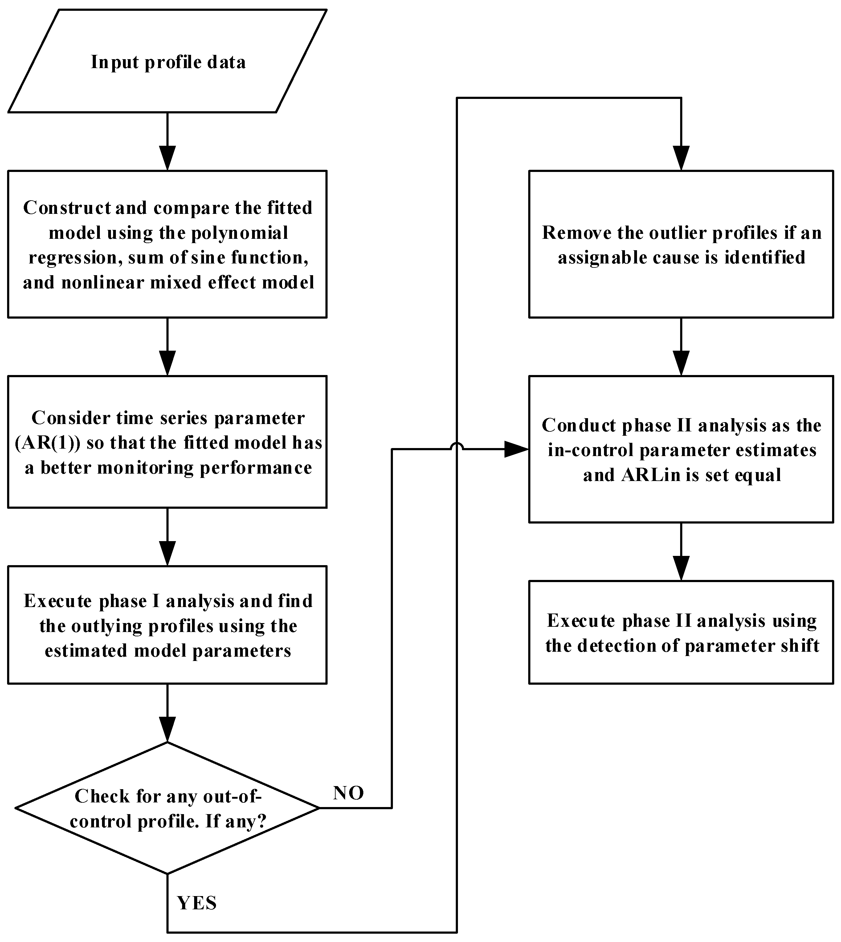
2. The Proposed Method for Monitoring Process Profiles

In the proposed framework, three different models are investigated to seek an appropriate profile model. Additionally, the Hotelling T² and the EWMA control charts are employed in order to monitor the profile shape and the profile residual, respectively. The flowchart is shown in Figure 1. First, the different process models are compared on the basis of $R_{adj}^2$, AIC_C, and SIC_C. According to the parameter estimates of the profile model, the nonlinear profile can be monitored and analyzed. In phase I, the Hotelling T² control chart is used to evaluate the process stability and remove any outlying profiles. The Hotelling T² control chart is also considered for phase II analysis via the out-of-control average run length (ARL_OUT). An EWMA control chart is utilized to check the residuals of the fitted model if the autocorrelation effect is changed or not.

2.1. Constructing the Profile Model

To evaluate and determine an appropriate process model, $R_{adj}^2$ is firstly considered to be an immediate measure so that the fitted performance can be more quickly compared. However, the performance evaluation of model fitting merely considers $R_{adj}^2$ that can cause the problem of overfitting. Hurvich and Tsai [12] had pointed out that the AIC would generate the overfitting problem when the fitting samples belong to a smaller number. Although Hurvich and Tsai [12] claimed that the AIC_C could enhance the accuracy of model selection, the overfitting problem can still occur to circumvent better estimation solutions. When referring to [13], we can find that the SIC_C seems to be able to deal with the overfitting problem for the small sample case. To deal with the accuracy of model selection and the overfitting problem, in this paper, the AICc and SICc are simultaneously adopted, with the expectation of obtaining adequate results. The small sample SIC_c and AIC_c criteria derived by [13] are described, as follows:

$${\mathrm{SIC}}_c=\log ({\widehat{\sigma }}_k^2)+\frac{\log (n)k}{n-k-2}$$

(1)

$${\mathrm{AIC}}_c=\log ({\widehat{\sigma }}_k^2)+\frac{n+k}{n-k-2}$$

(2)

In (1) and (2), the variance estimate is denoted by ${\widehat{\sigma }}_k^2={\displaystyle \sum _{j=1}^n{(y_j-{\widehat{y}}_j)}^2}/(n-1)$. Here, k is the number of the parameters in the process model. The number of measurement points that are in the profile is denoted by $n$. It is of particular importance to note that the variance estimate ${\widehat{\sigma }}_k^2$ is calculated after the autocorrelation effect has been discounted by using the first-order autoregressive model, which will be addressed shortly.

2.1.1. Polynomial Model

The polynomial model with one input variable can be defined by

$$y_{jp}={{\mathsf{\beta }}^{\prime }}_p{\mathbf{x}}_j+{\eta }_{jp},p=1,\dots ,q;j=1,\dots ,n$$

(3)

where the first-order autoregressive model is defined by ${\eta }_{jp}=\varphi {\eta }_{j-1,p}+{\epsilon }_{jp}$, which is logical in deeming the profile as a time series data set. Since the autocorrelation effect often occurs in profile monitoring, the first-order autoregressive model (i.e., AR(1)) is considered as the disturbance term, $\eta$, and is incorporated into the profile model. Therefore, the profile model will include the first-order autoregressive parameter to compensate. The parameter $\varphi$ is the first-order autoregressive (AR(1)) coefficient. The noise ${\epsilon }_{jp}$ is the error term of white noise and its variance estimate is indicated by ${\widehat{\sigma }}_k^2$, as in Equations (1) and (2). Also, ${{\mathsf{\beta }}^{\prime }}_p=\left[{\beta }_{0p},{\beta }_{1p},\dots ,{\beta }_{rp}\right]$ is the vector of unknown parameters in the polynomial function, the vector of regressors is denoted by ${{\mathbf{x}}^{\prime }}_j=\left[1,x_j,x_j^2,\dots ,x_j^r\right]$ and r denotes the order of the model in (3). Note that all of the parameters in Equation (3) are estimated by using the ordinary least squares estimation method (see [11]).

2.1.2. Model of the Modified Sum of Sine Functions in two Different Forms

The modified sum of sine functions is represented in the original form as

$$y_{jp}={\displaystyle \sum _{r=1}^k{\mathbf{a}}_{rp}\sin \left({\mathbf{b}}_{rp}{\mathbf{x}}_j+{\mathbf{c}}_{rp}\right)+{\eta }_{jp},r=1,\dots ,k;p=1,\dots ,q;j=1,\dots ,n}$$

(4)

where ${\mathbf{a}}_r$ is the amplitude, ${\mathbf{b}}_r$ is the frequency, and ${\mathbf{c}}_r$ is the horizontal phase constant at each sine wave term. For example, when the profile model is considered as the modified sum of two-sine functions, then the model can be defined by

$$y_{jp}=a_{1p}\sin (b_{1p}{x}_j+c_{1p})+a_{2p}\sin (b_{2p}{x}_j+c_{2p})+{\eta }_{jp}$$

(5)

where $x_j$ denotes the input variable for the jth measurement, ${\mathsf{\beta }}_p$ denotes the parameter vector in profile p (${{\mathsf{\beta }}^{\prime }}_p=[a_{1p},a_{2p},b_{1p},b_{2p},c_{1p},c_{2p}]$), and the ${\eta }_{jp}$ term is defined, as in Equation (3). As mentioned above, the parameters $a_1$ and $a_2$ are the amplitude of the function, $b_1$ and $b_2$ determine the period, and $c_1$ and $c_2$ influences the horizontal shift. The parameter estimation is performed by using the nonlinear least squares estimation method (see [11]).

To strengthen the fitting of nonlinear models by means of the modified sum of sine functions, we also use the nonlinear mixed effects model (NLME) to test the fitted performance, which then is extended into a nonlinear model with random effects. The generic form of NLME is given by the following equation:

$$y_{jp}=f({\mathsf{\beta }}_{jp},{\mathbf{x}}_j)+{\epsilon }_{jp},{\mathsf{\beta }}_{jp}={\mathbf{A}}_{jp}\mathsf{\theta }+{\mathbf{B}}_{jp}{\gamma }_{jp},p=1,\dots ,q,j=1,\dots ,n$$

(6)

In (6), $f$ is the function governing within-profile behavior, ${\mathsf{\beta }}_{jp}$ is a vector of group-specific model parameters, ${\mathbf{A}}_{jp}$ is a design matrix for combining fixed effects, $\mathsf{\theta }$ is a vector of fixed effects, ${\mathbf{B}}_{jp}$ is a design matrix for combining random effects, ${\gamma }_{jp}$ is a vector of multivariate normally distributed random effects with ${\gamma }_{jp}~N(0,\mathbf{D})$, where D is a covariance matrix for the random effects, and ${\epsilon }_{jp}$ is a vector of errors, which is assumed to be independent, identically, normally distributed, and independent of ${\gamma }_{jp}$, ${\epsilon }_{jp}~N(0,{\sigma }^2)$.

According to the mixed model that $\mathsf{\beta }=\mathbf{A}\cdot Fixedeffect+\mathbf{B}\cdot Randomeffect$, the estimated profile parameters ($\mathsf{\beta }$) of the two-sine function in terms of the NLME model can be described in Equation (7):

$$\left[\begin{array}{l}{a}_{1p}\\ b_{1p}\\ c_{1p}\\ a_{2p}\\ b_{2p}\\ c_{2p}\end{array}\right]=\mathbf{A}\cdot \left[\begin{array}{l}{\overline{a}}_1\\ {\overline{b}}_1\\ {\overline{c}}_1\\ {\overline{a}}_2\\ {\overline{b}}_2\\ {\overline{c}}_2\end{array}\right]+\mathbf{B}\cdot \left[\begin{array}{l}{a}_{1p}-{\overline{a}}_1\\ b_{1p}-{\overline{b}}_1\\ c_{1p}-{\overline{c}}_1\\ a_{2p}-{\overline{a}}_2\\ b_{2p}-{\overline{b}}_2\\ c_{2p}-{\overline{c}}_2\end{array}\right]$$

(7)

In Equation (7), the A and B are assumed to be the $1$ matrix, the bar symbol refers to an average. The NLME form can then be represented, as follows:

$$\begin{array}{lll}{y}_{jp}& =& [{\overline{a}}_1+(a_{1p}-{\overline{a}}_1)]\sin [({\overline{b}}_1+(b_{1p}-{\overline{b}}_1)x_j)+({\overline{c}}_1+(c_{1p}-{\overline{c}}_1))]+\\ & & [{\overline{a}}_2+(a_{2p}-{\overline{a}}_2)]\sin [({\overline{b}}_2+(b_{2p}-{\overline{b}}_2)x_j)+({\overline{c}}_2+(c_{2p}-{\overline{c}}_2))]+{\epsilon }_{jp}\\ & =& (a_{1,fixed}+a_{1p,random})\sin ((b_{1,fixed}+b_{1p,random})x_{ij}+(c_{1,fixed}+c_{1p,random}))+\\ & & (a_{2,fixed}+a_{2p,random})\sin ((b_{2,fixed}+b_{2p,random})x_{ij}+c_{2,fixed})+{\epsilon }_{jp}\end{array}$$

(8)

The parameter estimates are obtained by using the maximum likelihood estimation method (see [2]). Herein, it should be noted that the NLME model does not include the AR(1) term. In previous literature (see [2]), the NLME model has been used to solve the problem of autocorrelation. Therefore, the two fitting models together with AR(1) and the NLME model are compared in phase I analysis.

2.2. Phase I and II Monitoring and Analysis

In phases I and II, the parametric T² control chart is used to check whether the process is in the statistical control status and to identify potential outliers. Here, ${\widehat{\mathsf{\beta }}}_p$ is the estimate of the parameter vector. Over the entire profile data, the sample mean vector $\overline{\widehat{\mathsf{\beta }}}$ and the sample variance-covariance matrix $\mathbf{S}={\mathbf{s}}^2\left\{\widehat{\mathsf{\beta }}\right\}$ can be computed by using the parameter estimates that were obtained from different fitting models. For example, the estimate of the parameter vector for the fourth order polynomial with AR(1) is defined as $\left[\begin{array}{cccccc}{\widehat{\beta }}_0& {\widehat{\beta }}_1& {\widehat{\beta }}_2& {\widehat{\beta }}_3& {\widehat{\beta }}_4& \widehat{\varphi }\end{array}\right]$; the estimate of the parameter vector for the sum of two-sine functions with AR(1) is defined as $\left[\begin{array}{ccccccc}{\widehat{a}}_1& {\widehat{a}}_2& {\widehat{b}}_1& {\widehat{b}}_2& {\widehat{c}}_1& {\widehat{c}}_2& \widehat{\varphi }\end{array}\right]$.

According to the aforementioned parameter estimates, the T2 control chart (Brill, 2001) is described by

$$T_{c,p}^2=({\widehat{\mathsf{\beta }}}_p-\overline{\widehat{\mathsf{\beta }}}{)}^{\prime }{\mathbf{S}}_c^{-1}({\widehat{\mathsf{\beta }}}_p-\overline{\widehat{\mathsf{\beta }}}),p=1,2,\dots ,q,$$

(9)

where ${\mathbf{S}}_c$ is the sample variance-covariance estimator, as defined by

$${\mathbf{S}}_c=\frac{1}{q-1}{\displaystyle \sum _{p=1}^q({\widehat{\mathsf{\beta }}}_p-\overline{\widehat{\mathsf{\beta }}})({\widehat{\mathsf{\beta }}}_p-\overline{\widehat{\mathsf{\beta }}}{)}^{\prime }}$$

(10)

In (10), q is the number of profiles in the process data. The approximate upper control limit (UCL), as derived by [14], is as follows:

$${\mathrm{UCL}}_c=\frac{{(q-1)}^2}{q}{B}_{\alpha ,k/2,(q-k-1)/2}$$

(11)

In Equation (11), $B_{\alpha ,k/2,(q-k-1)/2}$ is the upper $\alpha$ percentage point of a beta distribution with parameters $k/2$ and $(q-k-1)/2$, where k is the number of parameter estimates. According to [15], the T² control chart in (9) is shown to be ineffective in detecting sustained shifts in the mean vector. In this regard, the alternative T² control chart that was proposed by [16] is also considered. The control chart is defined by

$$T_{D,p}^2=({\widehat{\mathsf{\beta }}}_p-\overline{\widehat{\mathsf{\beta }}}{)}^{\prime }{\mathbf{S}}_D^{-1}({\widehat{\mathsf{\beta }}}_p-\overline{\widehat{\mathsf{\beta }}}),p=1,2,\dots ,q$$

(12)

In (12), the variance-covariance estimator (${\mathbf{S}}_D$) is calculated by using successive differences in the following:

$${\mathbf{S}}_D=\frac{{\widehat{\mathbf{V}}}^{\prime }\widehat{\mathbf{V}}}{2(q-1)}$$

(13)

where ${\widehat{\mathbf{v}}}_p={\widehat{\mathsf{\beta }}}_{p+1}-{\widehat{\mathsf{\beta }}}_p$ for $p=1,\dots ,q-1$ and the transpose of these $q-1$ difference vectors are stacked into the $(q-1)\times k$ matrix $\widehat{\mathbf{V}}$, as follows:

$$\widehat{\mathbf{V}}=[{{\widehat{\mathbf{v}}}^{\prime }}_1{{\widehat{\mathbf{v}}}^{\prime }}_2\cdots {{\widehat{\mathbf{v}}}^{\prime }}_{q-1}{]}^{\prime }$$

(14)

In [17], the approximate UCLD for a large sample size ($q>k^2+3k$) can be estimated according to

$${\mathrm{UCL}}_D={\chi }^2(1-\alpha ,k),$$

(15)

where k denotes the degrees of freedom and $\alpha$ denotes the significance level. Sullivan and Woodall [15] argue that the simulation results can be used to discover that the $T_C^2$ control chart (see Equation (9)) performs worse in detecting the step change and the ramp shift in the mean vector during phase I than the $T_D^2$ chart, as shown in (12). Based on this fact, in this paper, the $T_D^2$ control chart is employed to evaluate the different fitting models while identifying the outlying profiles.

While phase I is executed, the process should be able to achieve a stable situation. Subsequently, the data of the in-control profiles is employed to estimate the unknown parameters. In phase II, the exponentially weighted moving average (EWMA) chart is additionally used for detecting the autoregressive (AR) effect in residuals in order to determine whether the AR parameter in the process model should be re-estimated. In sum, the $T_D^2$ control chart is used to monitor the parameters of the model (i.e., profile shape). In the meantime, the EWMA control chart is used to monitor the residuals (i.e., profile variability). The EWMA statistic is computed by

$${\mathrm{EWMA}}_{\epsilon }(j)=\theta e_j+(1-\theta ){\mathrm{EWMA}}_{\epsilon }(j-1),j=1,2,\dots ,n,$$

(16)

where $e_j$ is the $j\mathrm{th}$ residual; $\theta (0<\theta \le 1)$ is a smoothing constant and the starting value is assumed ${\mathrm{EWMA}}_{\epsilon }(0)=0$. An out-of-control signal is issued as soon as ${\mathrm{EWMA}}_{\epsilon }(j)<LCL$ or ${\mathrm{EWMA}}_{\epsilon }(j)>UCL$, where

$$LCL=0-L_{\epsilon }{\widehat{\sigma }}_{\epsilon }\sqrt{\frac{\theta }{2-\theta }},UCL=0+L_{\epsilon }{\widehat{\sigma }}_{\epsilon }\sqrt{\frac{\theta }{2-\theta }}$$

(17)

In (17), ${\widehat{\sigma }}_{\epsilon }$ denotes the standard error of the residual as ${\widehat{\sigma }}_k$ in Equations (1) and (2); $L_{\epsilon }(>0)$ is a half-length that is designed to generate a specific in-control ARL. Under this monitoring framework, the ARL_OUT performance of the T² control chart, together with the EWMA chart, is evaluated for phase II analysis in the next section. In terms of the aforementioned methods, the proposed monitoring framework can be formalized as pseudo-code 1 in the appendix.

3. Experimental Results for Profile Monitoring

In this section, the proposed monitoring framework is illustrated and evaluated while using the simulated reflow process in SMT. The application domains of the monitoring system and some implementation issues are discussed. In terms of the simulation results, the analysis of profile monitoring can be done in three parts: (i) making a comparison of the fitting performance between the polynomial regression with AR(1), the modified sum of sine functions with AR(1), and the NLME model; (ii) screening the outlying profiles by means of the $T_D^2$ control chart for phase I analysis; and, (iii) testing the proposed $T_D^2$ control chart with the EWMA control chart, while also monitoring the process parameters and the residual in phase II analysis.

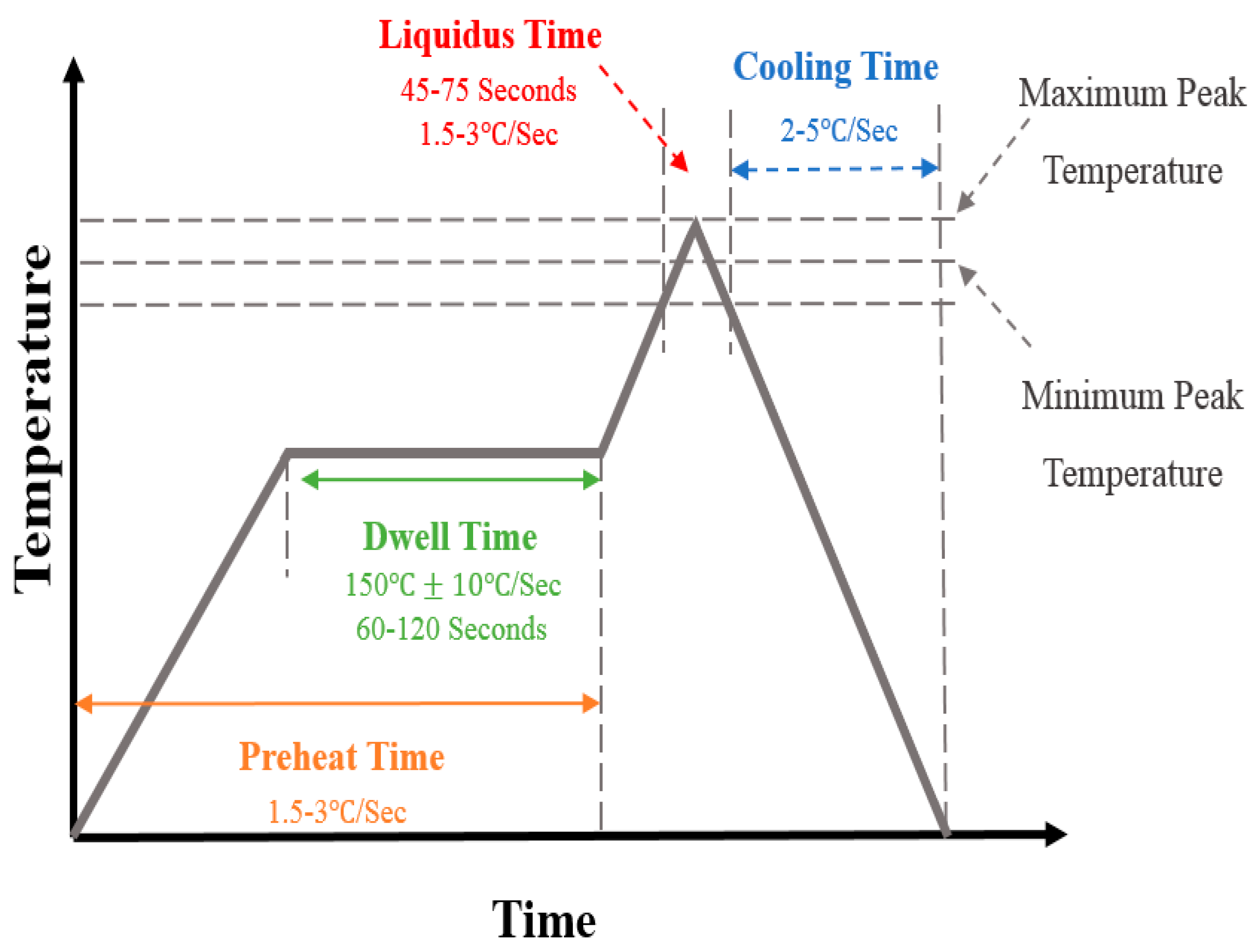
3.1. Fundamentals of Reflow Process

The operation of the reflow process is the heating sequence for assembling printed circuit boards (PCB) using solder paste at successively higher temperatures. As an assembly moves through a soldering system, it will perform a controlled temperature curve in order to achieve the required quality. Such a temperature curve is also called a “temperature profile”. The temperature profile is often measured along a variety of technical dimensions, such as slope, soak, time above liquidus, and peak. In general, reflow soldering processes contain four stages. Each operation presents a unique temperature profile: preheat, thermal soak (dwell), reflow (liquidus), and cooling. Figure 2 shows a typical example of a schematic temperature profile.

In the preheat zone step, the changes of the temperature curve can be described as an ascending tendency from normal temperature to approximately 150 °C. In this step, the ascending temperature facilitates the removal of solvent and water vapor in the solder paste. Rapid heating helps the flux softening temperature to be reached quickly, so the flux can spread quickly and cover the maximum area of solder joints. It also integrates some activator into the actual alloy liquid. Furthermore, because some parts of the motherboard cannot deal with the sharp temperature changes, the rate of temperature change in the preheating zone is set to between 1.5 °C/s and 3 °C/s.

When the operation approaches the thermostatic zone, the temperature is usually maintained in a region of 150 ± 10 °C. This operational zone is a flat temperature profile to enhance the effect of the soldering, and it especially prevents tombstoning. The reflow zone is also called Time Above Liquidus (TAL). The TAL is the period of time above the maximum temperature at which crystals can coexist with the melt in thermodynamic equilibrium. The peak of reflow temperature usually depends on the melting temperature of the solder, while also taking into account the temperature that assembled components can endure. For instance, a typical lead-free manufacturing process must not exceed the limit of 260 °C, which is the highest temperature that tantalum capacitors can endure.

Following the reflow zone, the product is cooled and the solder joints are solidified so that it can rejoin the assembly process. Note that Figure 2 only provides an overall, schematic diagram of the temperature profile of the reflow process. In fact, the temperature control in the reflow process belongs to a nonlinear profile pattern. Hence, any linear approximation approach will not be suited to this research. The high nonlinearity and curvature somewhat warrants the need for a new profile monitoring approach. In this paper, the practical data of the same product type is gathered so as to form individual profiles for process monitoring. The production line in the SMT practice is essentially constructed with high flexibility to deal with the different types of products. Hence, to perform profile monitoring of a wide variety of low-volume products in small-to-moderate batches is our research target. Note that the data set that was used in this research is available upon request.

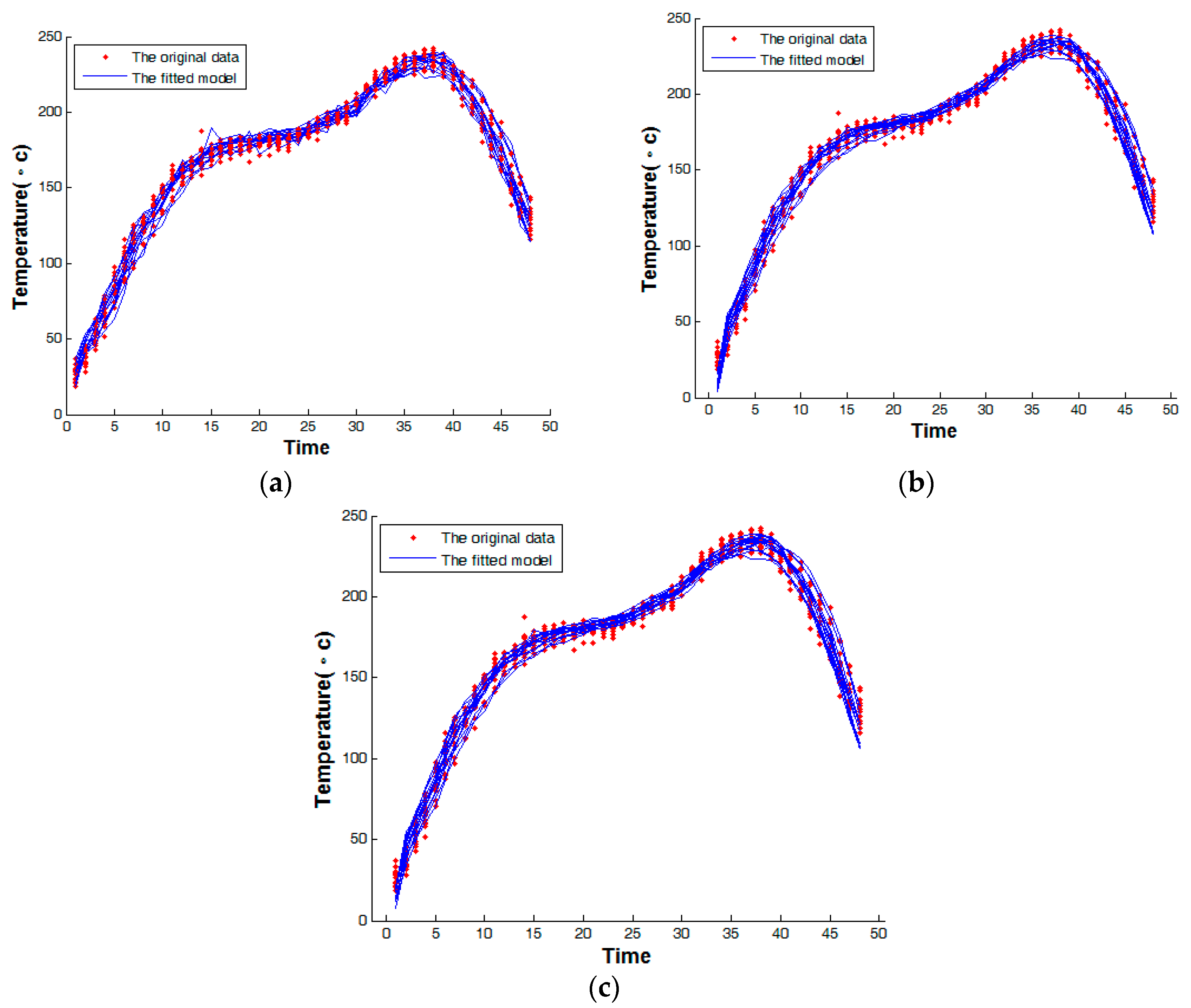
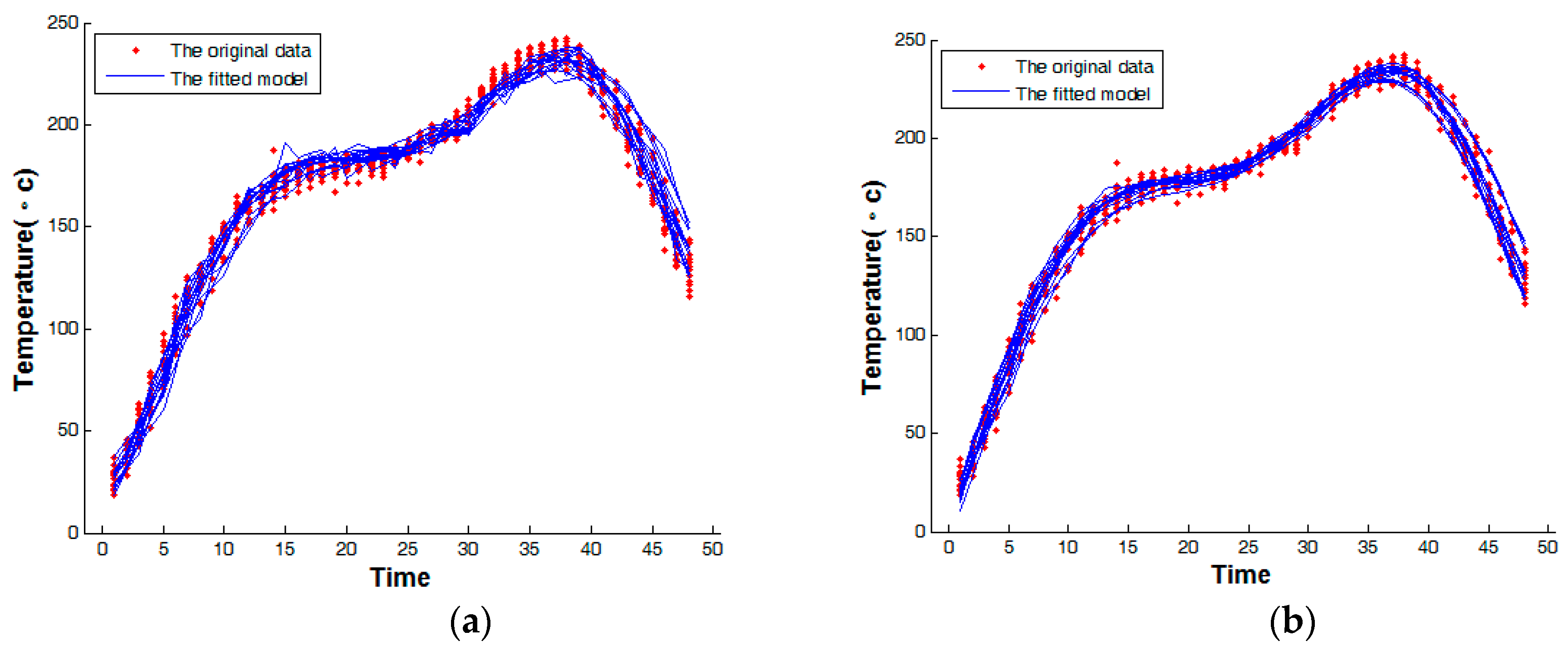
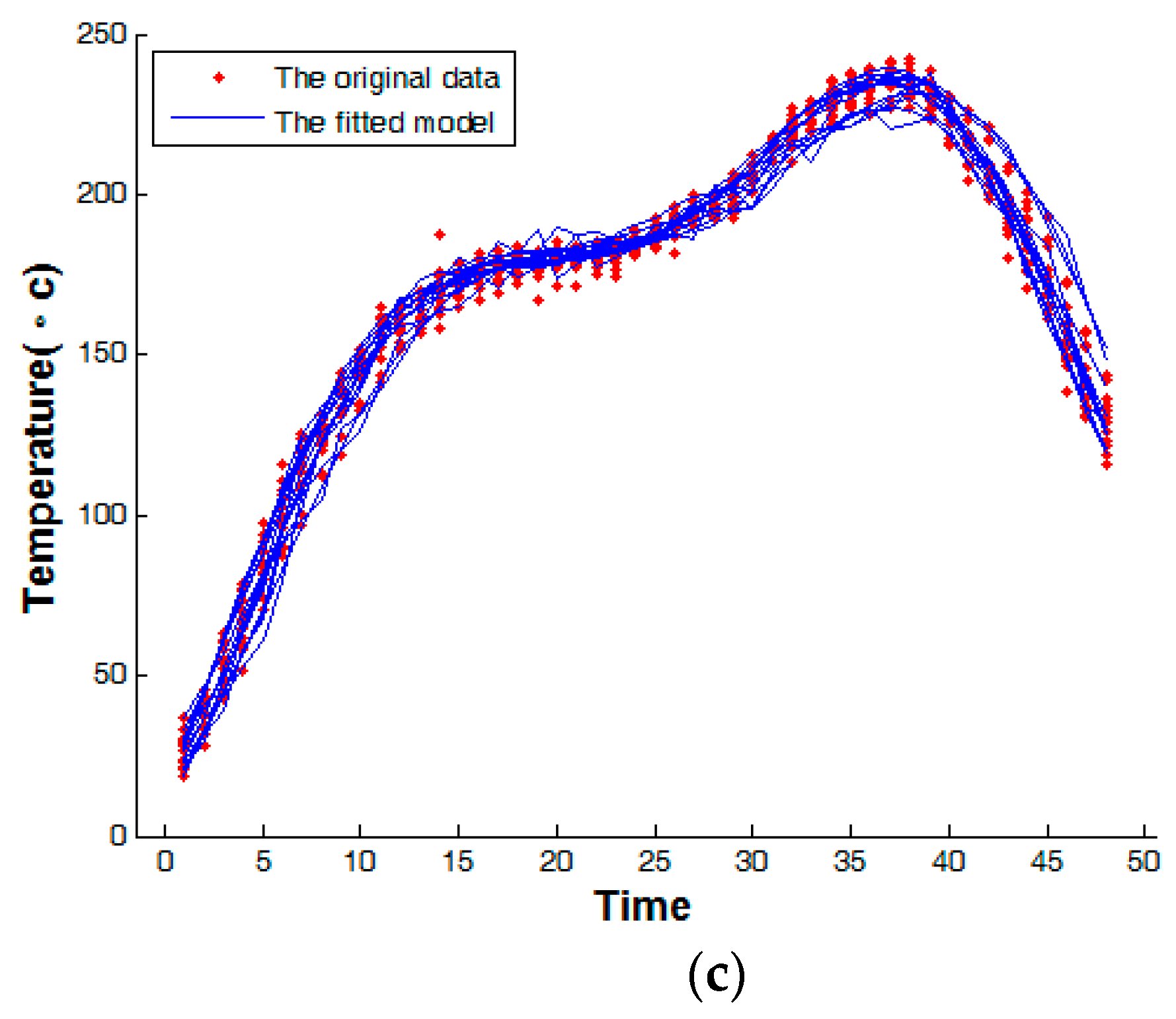
3.2. Comparing and Evaluating the Different Profile Models

In this section, the polynomial regression model, the modified sum of sine functions, and the NLME model are first used to fit the reflow process data. The polynomial models of orders 3–5 and the modified sum of 1–3 sine functions are selected for model fitting. In every profile, n measurements in the ith random profile are collected over time, as indicated by $(x_{jp},y_{jp})$, for $p=1,2,\dots ,q$ and $j=1,2,\dots ,n$. The polynomial models are as shown in Equation (3). The modified sum of sine functions and the nonlinear mixed effects models are as shown in Equations (4)–(7).

In here, seven models, including the polynomial model of different orders with AR(1), the modified sum of sine functions with AR(1), and the NLME model, are tested. Fifteen profiles of 48 data points that were collected each in the reflow process are individually modelled by using the seven different models, and the parameter estimates are utilized for phase I monitoring. To compare the fitting results, four performance measures ($R_{adj}^2$, RSS, $SI{C}_c$, and $AI{C}_c$) are selected as the performance measures. Moreover, the number of times that each model is chosen best over 15 profiles is also reported. The computational results are displayed in Table 1 and Figure 3, Figure 4 and Figure 5. From the fitting results in Table 1, it can be seen that the modified sum of two-sine functions exhibits a better fitting performance (with less SIC and AIC) than the other fitted models. Typically, using a large sample of profiles for parameter estimation in the phase I analysis is necessary, especially for nonlinear profiles. In this study, only fifteen profiles can be obtained due to a technical limitation. The excellent fitting performance that is shown in Table 1 and Figure 3, Figure 4 and Figure 5 must be attributed to the appropriateness of model selection and the flexibility of the chosen models under investigation. If the fitting performance is not satisfactory, then more profile data need to be collected for the estimation purpose before proceeding to the phase II analysis.

The particularly high performance based on the four measures arises from the suitability of the modified sum of two-sines with AR(1) for the reflow process data. Thus, the model previously mentioned is considered to be the best model to undertake research. The polynomial model of order 4 with AR(1) outperforms the other polynomial models, thus being considered as the benchmark model. These two process models with AR(1) show great flexibility in dealing with complex model-building situations, and therefore they are also expected to be extensively applied in a wide variety of nonlinear processes. They will be selected for evaluation in phase I and II monitoring.

3.3. Simulations for Phase I Analyses

In phase I, following [18] and [16], the $T_D^2$ chart is used for identifying the outlying profiles. First, the statistic $T_D^2$ of the parameter estimates (including the AR(1) parameter) is calculated based on Equation (12). Based on the polynomial regression model of order 4 and the modified sum of two-sines, the control limit of $T_D^2$ control chart is plotted in Figure 6. Since no outlying profiles are found in the 15 phase I runs, as in the common SPC practice, no profiles need to be removed prior to the phase II. On the other hand, three types of the hypothetical process abnormalities are also tested in order to assess and compare the performance of phase I monitoring. The first scenario assumes that the preheat zone has a lower temperature slope. The maintenance of temperature in the dwell zone is assumed to be unstable for the second scenario, and in the third scenario the temperature is set to over-heating in the reflow zone. Figure 7 shows the three outlying profiles along with the average baseline using 15 in-control profiles. In common practice, these three types of abnormality will not happen at the same time. Accordingly, in our paper, we test each abnormal profile separately.

In this simulation, the significance level of $\alpha =0.05$ is used as the significance level for any individual profile, i.e., $T_p^2,p=1,\dots ,15$, and to construct the control limits [14,17]. The three simulated abnormal profiles are individually added to the 15 in-control profiles. The $T_D^2$ statistic is computed for the polynomial regression and the modified sum of two-sine functions with the AR(1) model. Figure 8 and Figure 9 show the monitoring results of the $T_D^2$ control charts for abnormal profiles 1, 2, and 3. The simulated results reveal that the $T_D^2$ control charts are able to identify the outlying situations if the abnormal profiles are present. It is worth to note that the $T_D^2$ control chart is like a moving range with individual observations, and it is not affected by shifts in the mean vector, and as a result of which it has greater power.

The polynomial model of order 4 with AR(1) and the modified sum of two-sine functions with AR(1) can account for the autocorrelation effects appropriately, so the simulated abnormal profiles can be successfully detected. From a fitting performance viewpoint based on Table 1, the modified sum of two-sine functions with AR(1) takes the lead between the compared models. From an operational point of view, the polynomial model of order 4 can be adopted, since it contains fewer unknown parameters to be estimated and it is easier to implement in practice than the modified sum of two-sine functions. By contrast, the modified sum of two-sine functions explains the data variance better and is more powerful than the polynomial model of order 4. Therefore, during the pre-production stage where the process insights should be fully gained for the purpose of process adjustment/optimization, the modified sum of two-sine functions can be considered instead.

3.4. Simulation Results for Phase II Monitoring

The objective of phase II is to detect shifts quickly in the process. The reliable control limits can be established to achieve effective on-line monitoring in phase II when the in-control process data is stable. The proposed monitoring framework uses the composite method to monitor two possible process irregularities. First, the $T_D^2$ control chart is applied, so that the profile shape of the fitted model can be monitored. Second, the autocorrelation of residuals is monitored by using the EWMA control chart. If the process has been confirmed to be stable, then the 15 in-control profiles will be employed in order to estimate the parameters of the fitted model, the mean vector, and the variance-covariance. The parameter estimates are used to replace the unknown parameters in Equations (3)–(7), plus an error term to simulate the profile data. The practical process is assumed to follow the modified sum of two-sine functions with the error term to simulate the process changes. The variance of the fitted model is estimated by using the mean square error (MSE), over the 15 in-control profiles, from the model-building stage. The error term of the process model is assumed to be normally distributed with zero mean and constant variance. Next, the $T_D^2$ and EWMA control charts are employed to implement the phase II analysis, evaluating the detection performance as the process parameters shift. The control limits are constructed using the parameter estimates of the three different fitting models (the polynomial regression model of order 4 with AR(1), the modified sum of two-sine functions with AR(1), and the traditional polynomial regression model of order 4) to evaluate and compare the monitoring performances. The traditional polynomial regression model of order 4 is only used as a benchmark. To monitor the process shape on a fair basis, in each fitting model the different control limits should be particularly designed to have an approximately equal in-control ARL (i.e., ARL_IN = 100) when using 10,000 simulation cycles. Moreover, the smoothing constant ($\theta$) in the EWMA chart is set to 0.02, as in [11] and [19]. Here, in each experiment, 20,000 profiles are simulated for ARL_OUT evaluation in terms of the shifts of different scales in the six parameters of the modified sum of two-sine functions. Note that, based on an earlier experiment, using a typical ARL_IN in our study, like 370 or even larger, will cause indistinguishable performance in ARL_OUT in the presence of a small scale of parameter change. The formal procedure in the Phase II analysis is represented as pseudo-code 2 in the Appendix A.

In the ordinary SMT operation, if the process recipe is suitably tuned before volume production, then the profile specification should be pre-determined and only subjected to a minuscule adjustment as a result of product changes. Therefore, seven different types of shifts are considered in our simulation study. The shifts of these process parameters are applied to the amplitude, the frequency, and the horizontal phase constant in the model, as shown in Equation (5). The simulation results of ARL_OUT can be used to evaluate the on-line monitoring capability. These ARL_OUT values are calculated by setting equally spaced parameter shifts every 100 simulated profiles (maximum ${\mathrm{ARL}}_{\mathrm{IN}}=100$) and then averaging across 20,000 simulation cycles. The parameter shift in the scale of ${\sigma }_{\mathsf{\beta }}$ ranges from 0.5 to 3 for the six process parameters. Any parameter shift will cause the change of curve shape that is closest to the type of sustained shift in SPC practice. Figure 10a shows the comparative profiles under various shifts of different process parameters. In order to detect the autocorrelation effect in the residuals of each profile, the EWMA control chart is used to implement the related monitoring tasks using the different scales of the autocorrelation coefficient, from 0.1 to 0.9 (see Figure 10b).

Table 2 gives the ARL_OUT estimates for shifts of the six parameters. The experimental results indicate that, for monitoring the shape of the model, both of the composite models perform reasonably well regardless of whether the data is modeled by the modified sum of two-sine functions or the polynomial regression model. We also use the EWMA control chart to monitor residuals if any autocorrelation effect in addition to the AR(1) already included in the model is exhibited. The results show that the modified sum of two-sine functions, combined with AR(1), performs much better than the pure polynomial regression model as $\lambda \ge 1.5$. Even so, it is very difficult to compare the modified sum of two-sine functions and the polynomial regression model in the composite approach, although the former performs slightly better than the latter. In a word, it is reasonable to allege that the modified sum of two-sine functions can be a viable modeling option for nonlinear profiling monitoring circumstances where only small samples are available for the reflow process.

4. Conclusions

This paper presents a new monitoring framework for dealing with the autocorrelation effect that exists in the errors around the functional relationship when only small samples are available. The research framework includes model building and phase I and II analyses. The central idea of the proposal is how to construct an appropriate profile model that is capable of dealing with the time series effect. Using different profile models (the polynomial regression model, the modified sum of two-sine functions, and the nonlinear mixed effects model), the phase I and II analyses of reflow process data can be conducted. In phase I, the Hotelling $T_D^2$ control chart is utilized to screen the outlying profiles. When the outlying profiles are investigated and removed, then the same control charts with the EWMA control chart for monitoring autocorrelation are used for phase II monitoring, where the detectability of parameter shifts in terms of ARL_OUT is evaluated. According to the comparison results, some concluding remarks and suggestions can be provided:

• If the profile pattern exhibits a significant autocorrelation effect, then the proposed framework can use a different profile model with AR(1) and the proposed model selection procedure to strengthen the fitting performance. Furthermore, we feel safe to conclude that the sum of two-sine functions with AR(1) can be a viable modelling option for nonlinear profiling monitoring instances where only small samples are available for the reflow process.
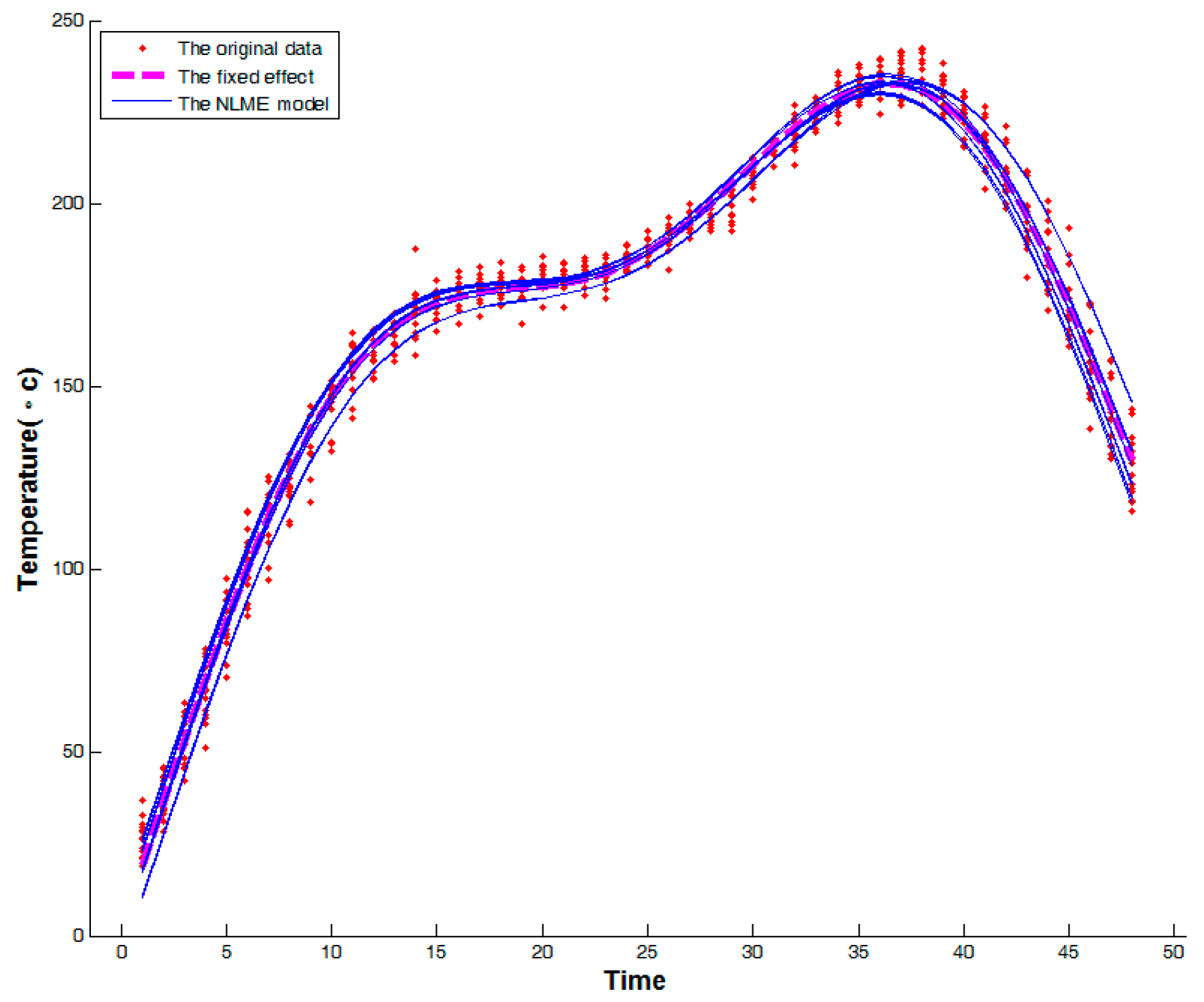
• In phase I of the reflow process that is investigated in this paper, two types of composite models all have good monitoring ability for identifying outlying profiles. However, the nonlinear mixed effects model cannot resolve the problem of autocorrelation in the residuals. This situation will cause difficulties in monitoring when autocorrelation is present.
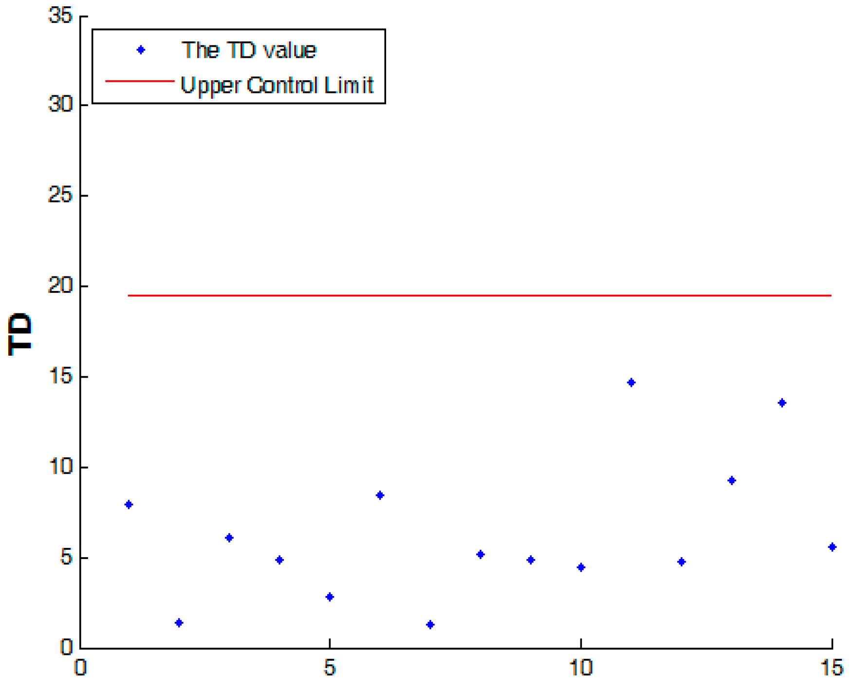
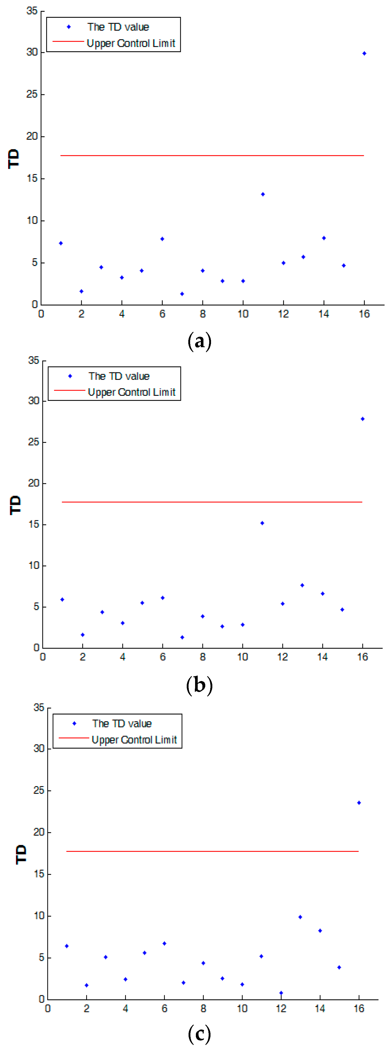
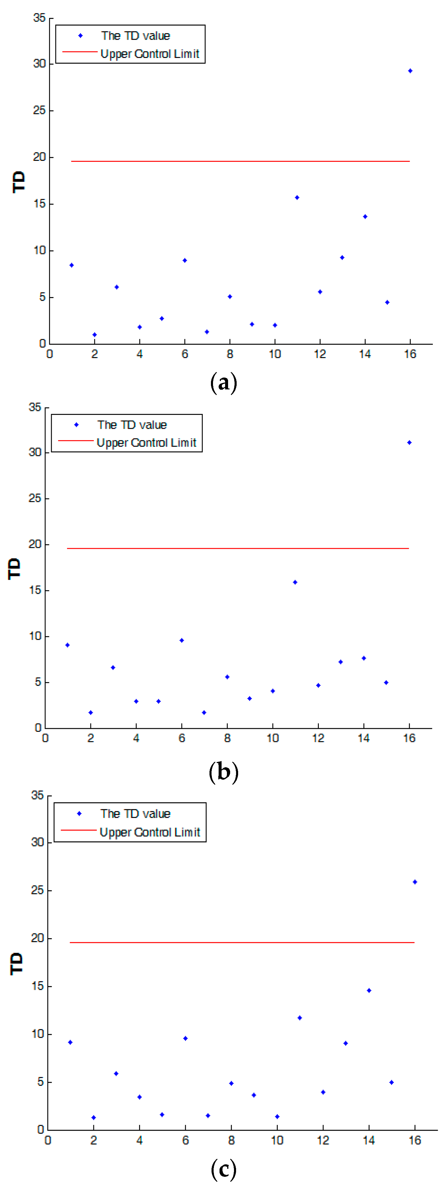
• According to the phase I results of the reflow process that was investigated in this study, the Hotelling T² control chart can produce satisfactory performance for monitoring of the process profile.
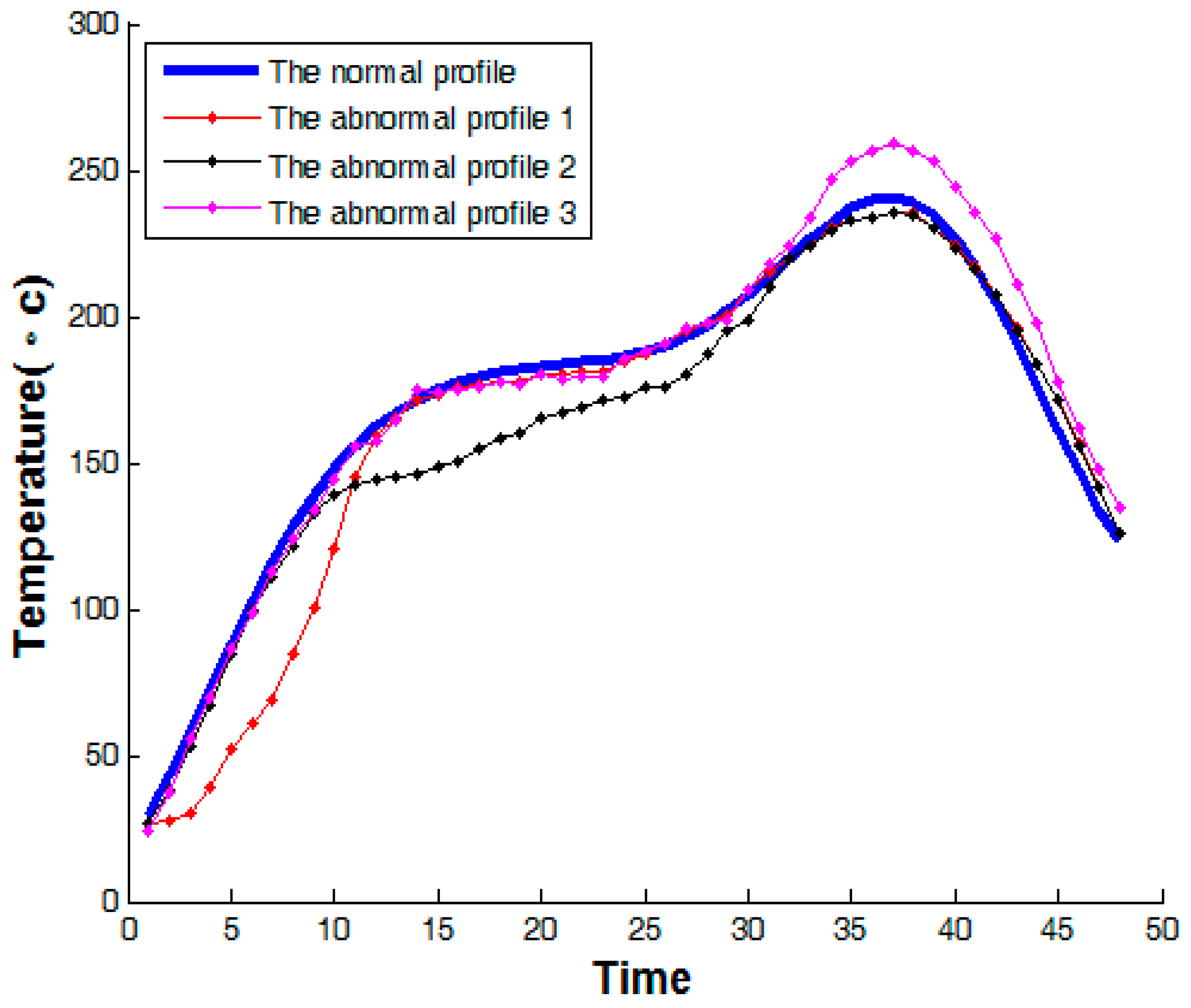
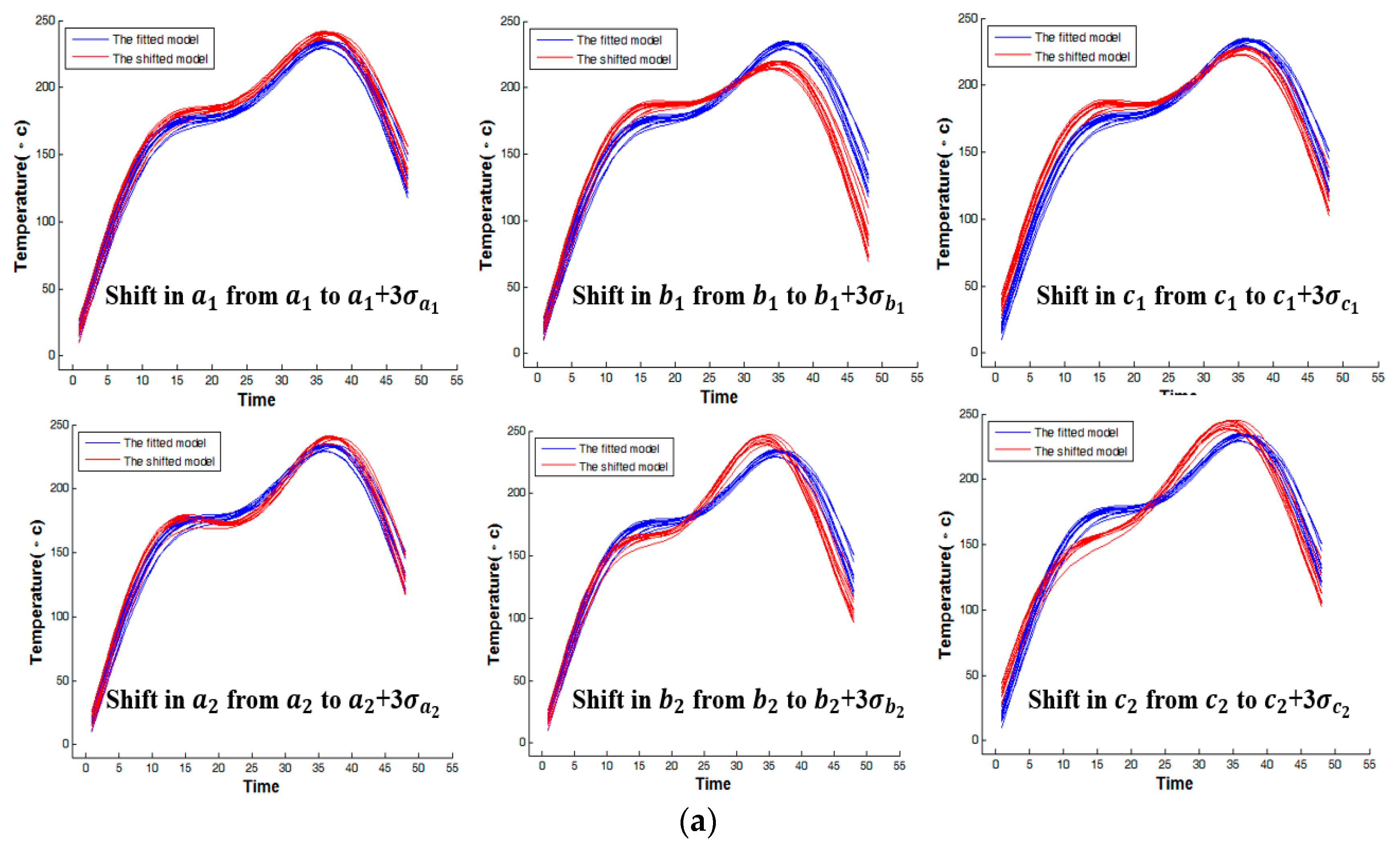
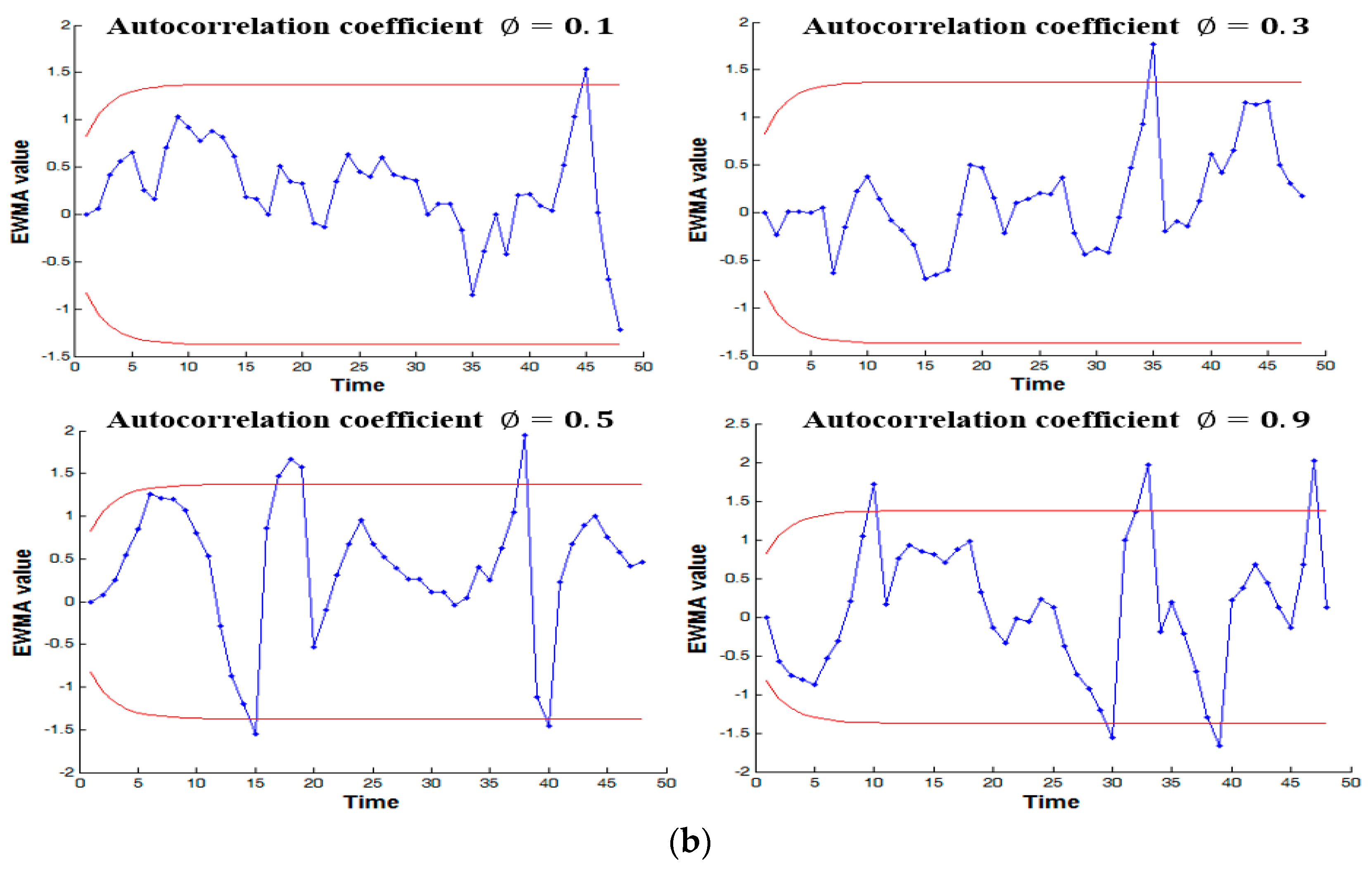
• On the whole, the proposed monitoring framework displays better detecting performances than the traditional polynomial regression model in phase II analysis for the reflow process that is discussed in this paper. In addition, the proposed EWMA control chart is also effective in detecting changes of the autocorrelation effect in residuals. This study pinpoints a major finding, a fact that the modified sum of two-sine functions is able to statistically fit the nonlinear profile of the reflow process data extremely well. In the proposed framework, the Hotelling T² control chart and the EWMA control chart work in harmony to simultaneously monitor the parameter estimates (i.e., profile shape) and residuals (i.e., profile variability), respectively. The simulation results in phases I and II illustrate the proposed monitoring framework. Therefore, the practitioner can follow the guidelines of model building and process monitoring that are demonstrated in this paper, as the nonlinear profile monitoring task of the reflow process is necessary.
• To achieve desirable monitoring performances for other potential applications, the parameter setting of the control chart bears further scrutiny. A real-data examination of phase II analysis should be further conducted to complement the research outcomes that are delivered in this paper.

References

1. Montgomery, D.C. Introduction to Statistical Quality Control, 5th ed.; Wiley: New York, NY, USA, 2005. [Google Scholar]
2. Jensen, W.A.; Birch, J.B.; Woodall, W.H. Monitoring correlation within linear profiles using mixed models. J. Qual. Technol. 2008, 40, 167–185. [Google Scholar] [CrossRef]
3. Chicken, E.; Pignatiello, J.J., Jr.; Simpson, J.R. Statistical process monitoring of nonlinear profiles using wavelets. J. Qual. Technol. 2009, 41, 198–212. [Google Scholar] [CrossRef]
4. Qiu, P.; Zou, C.; Wang, Z. Nonparametric profile monitoring by mixed effects modeling. Technometrics 2010, 52, 265–277. [Google Scholar] [CrossRef]
5. Hung, Y.C.; Tsai, W.C.; Yang, S.F.; Chuang, S.C.; Tseng, Y.K. Nonparametric profile monitoring in multi-dimensional data spaces. J. Process Control 2012, 22, 397–403. [Google Scholar] [CrossRef]
6. Chuang, S.C.; Hung, Y.C.; Tsai, W.C.; Yang, S.F. A framework for nonparametric profile monitoring. Comput. Ind. Eng. 2013, 64, 482–491. [Google Scholar] [CrossRef]
7. Ghahyazi, M.E.; Niaki, S.T.A.; Soleimani, P. On the monitoring of linear profiles in multistage processes. Qual. Reliab. Eng. Int. 2014, 30, 1035–1047. [Google Scholar] [CrossRef]
8. Zhang, Y.; He, Z.; Zhang, C.; Woodall, W.H. Control charts for monitoring linear profiles with within-profile correlation using Gaussian process models. Qual. Reliab. Eng. Int. 2014, 30, 487–501. [Google Scholar] [CrossRef]
9. Khedmati, M.; Niaki, S.T.A. Phase II monitoring of general linear profiles in the presence of between-profile autocorrelation. Qual. Reliab. Eng. Int. 2016, 32, 443–452. [Google Scholar] [CrossRef]
10. Jensen, W.A.; Grimshaw, S.D.; Espen, B. Nonlinear profile monitoring for oven-temperature data. J. Qual. Technol. 2016, 48, 84–97. [Google Scholar]
11. Fan, S.-K.S.; Chang, Y.J.; Aidara, N. Nonlinear profile monitoring of reflow process data based on the sum of sine functions. Qual. Reliab. Eng. Int. 2013, 29, 743–758. [Google Scholar] [CrossRef]
12. Hurvich, C.M.; Tsai, C.L. Regression and time series model selection in small samples. Biometrika 1989, 76, 297–307. [Google Scholar] [CrossRef]
13. McQuarrie, A.D. A small-sample correction for the Schwarz SIC model selection criterion. Stat. Prob. Lett. 1999, 44, 79–86. [Google Scholar] [CrossRef]
14. Tracy, N.D.; Young, J.C.; Mason, R.I. Multivariate control charts for individual observations. J. Qual. Technol. 1992, 24, 88–95. [Google Scholar] [CrossRef]
15. Sullivan, J.H.; Woodall, W.H. A comparison of multivariate control charts for individual observations. J. Qual. Technol. 1996, 28, 398–408. [Google Scholar] [CrossRef]
16. Holmes, D.S.; Mergen, A.E. Improving the performance of the T2 control chart. Qual. Eng. 1993, 5, 619–625. [Google Scholar] [CrossRef]
17. Williams, J.D.; Woodall, W.H.; Birch, J.B. Statistical monitoring of nonlinear product and process quality profiles. Qual. Reliab. Eng. Int. 2007, 23, 925–941. [Google Scholar] [CrossRef] [Green Version]
18. Brill, R.V. A case study for control charting a product quality measure that is a continuous function over time. Presented at the 45th Annual Fall Technical Conference, Toronto, ON, Canada, 18–19 October 2001. [Google Scholar]
19. Kim, K.; Mahmoud, M.A.; Woodall, W.H. On the monitoring of linear profile. J. Qual. Technol. 2003, 35, 317–328. [Google Scholar] [CrossRef]
Figure 1. Flow chart for the proposed framework.
Processes 07 00104 g001
Figure 2. A typical temperature profile.
Processes 07 00104 g002
Figure 3. The fitting profile using the polynomial with AR(1) model. (a) The third-order model; (b) The fourth-order model; and, (c) The fifth-order model.
Processes 07 00104 g003
Figure 4. The fitting profile using the sum of sine model with AR(1) model. (a) The one-sine model; (b) The two-sine model; a d, (c) The three-sine model.
Processes 07 00104 g004aProcesses 07 00104 g004b
Figure 5. The fitted profiles of the nonlinear mixed effects model (NLME).
Processes 07 00104 g005
Figure 6. T D 2 control chart of the sum of two-sine function by using the fifteen in-control profiles.
Processes 07 00104 g006
Figure 7. The simulations of abnormal profiles.
Processes 07 00104 g007
Figure 8. Detect the abnormal profiles using the polynomial model with the 16 profiles (fifteen in-control and one out-of-control for each scenario). (a) Detecting the abnormal profile 1; (b) Detecting the abnormal profile 2; and, (c) Detecting the abnormal profile 3.
Processes 07 00104 g008
Figure 9. Detect the abnormal profiles using the sum of sine function with the 15 in-control profiles. (a) Detecting the abnormal profile 1; (b) Detecting the abnormal profile 2; and, (c) Detecting the abnormal profile 3.
Processes 07 00104 g009
Figure 10. Phase II analysis. (a) Detecting the curve changes using different shifts of process parameters; and, (b) Detecting the autocorrelation effect of residuals using exponentially weighted moving average (EWMA) control chart.
Processes 07 00104 g010aProcesses 07 00104 g010b