Article

Precise Lightning Strike Detection in Overhead Lines Using KL-VMD and PE-SGMD Innovations

1
Xinjiang Electric Power Research Institute, State Grid Xinjiang Electric Power Co., Ltd., Urumqi 830011, China
2
Key Laboratory of Renewable Energy Power Generation and Grid-Connected Technology in the Autonomous Region, Xinjiang University, Urumqi 830017, China
3
Engineering Research Center of Renewable Energy Power Generation and Grid-Connected Control, Ministry of Education, Xinjiang University, Urumqi 830017, China
4
Turpan Power Supply Company, State Grid Xinjiang Electric Power Co., Ltd., Turpan 838000, China
5
Altay Power Supply Company, State Grid Xinjiang Electric Power Co., Ltd., Altay 836500, China
*
Author to whom correspondence should be addressed.
Processes 2024, 12(2), 329; https://doi.org/10.3390/pr12020329
Submission received: 7 January 2024 / Revised: 26 January 2024 / Accepted: 1 February 2024 / Published: 2 February 2024

Abstract

:
When overhead lines are impacted by lightning, the traveling wave of the fault contains a wealth of fault information. The accurate extraction of feature quantities from transient components and their classification are fundamental to the identification of lightning faults. The extraction process may involve modal aliasing, optimal wavelet base issues, and inconsistencies between the lightning strike distance and the fault point. These factors have the potential to impact the effectiveness of recognition. This paper presents a method for identifying lightning strike faults by utilizing Kullback–Leibler (KL) divergence enhanced Variational Mode Decomposition (VMD) and Symmetric Geometry Mode Decomposition (SGMD) improved with Permutation Entropy (PE) to address the aforementioned issues. A model of a 220 kV overhead line is constructed using real faults to replicate scenarios of winding strike, counterstrike, and short circuit. The three-phase voltage is chosen and then subjected to Karenbaren decoupling in order to transform it into zero mode, line mode 1, and line mode 2. The zero-mode voltage is decomposed using KL-VMD and PE-SGMD methods, and the lightning identification criteria are developed based on various transient energy ratios. The research findings demonstrate that the criteria effectively differentiate between winding strike, counterstrike, and short-circuit faults, thus confirming the accuracy and efficacy of the lightning fault identification criteria utilizing KL-VMD and PE-SGMD.

1. Introduction

High-voltage overhead lines serve as the primary conduits for the transmission of electric power and constitute a crucial component of the power grid [1,2]. These entities are situated in expansive regions with diverse natural and geographical features, rendering them particularly vulnerable to lightning strikes. More than 50% of power system accidents in Japan result from lightning strikes on transmission lines. In nations such as the former Soviet Union and the United States, 60% of incidents involving 275–500 kV overhead lines are attributed to lightning strikes. In China, lightning strikes account for 40% to 70% of all trip accidents [3]. The transient stage of the fault contains abundant fault information [4]. The accurate detection of signal anomalies and the extraction of feature from complex transient components are vital for the prompt and precise identification of the fault type in power systems. This is essential to maintain their stable operation.
Concurrently, a significant body of research has been dedicated to the development of feature extraction and identification methods for lightning strikes on transmission lines. Identification methods primarily rely on two aspects: the high-frequency transient components and the amplitude of lightning. Depending on the approach to feature extraction, the primary methods for identifying lightning strikes include the amplitude method, time-domain waveform method, modal extremum method, wavelet energy spectrum method, and high-frequency attenuation ratio method.
Zou et al. [5] suggest that the mutation points of transient traveling waves correspond one-to-one with the wavelet transform modulus maxima points. The strength of the traveling wave changes is characterized by the magnitude of the wavelet modulus, whereas the direction of the signal change is indicated by the polarity of the wavelet changes. Consequently, the wavelet transform modulus maxima can be utilized for the identification of the type of lightning strike. Shu et al. [6] propose a method for distinguishing between non-fault lightning strike currents and fault traveling waves. This method involves comparing the maximum initial modulus and the maximum second modulus of transient traveling waves. This comparison helps in identifying whether the waves are truncated by the fault point (i.e., a fault traveling wave) or not truncated (i.e., a non-fault lightning strike current). This approach aids in the identification of non-fault and fault lightning strikes. Sima et al. [7] utilize wavelet transform modulus maxima for the identification of the polarity of initial transient voltage surges and the duration of surge arrester discharge. This is achieved by analyzing the polarity of the wavelet modulus maxima and discharge time to detect winding strike and counterstrike faults. Guo et al. [8] differentiate between short-circuit and lightning faults by analyzing their high-frequency distribution. This is achieved by using the modulus maxima of the detail coefficients obtained through wavelet transform as criteria. These identification methods [5,6,7,8] exhibit high reliability and remain unaffected by the initial phase angle of the fault, the type of fault, and the transient fault resistance. However, the identification of modulus maxima presents a challenge and lacks a standardized approach.
Zhong et al. [9] utilize mathematical morphology for the analysis of variations in fault waveforms. It compares the clustering effects of single-scale and multi-scale fractal curves to classify and identify lightning faults. Si et al. [10] employ a linear regression to model the disturbed traveling wave by analyzing the variations in the waveform of the transient traveling wave over time. The fit is satisfactory for cases of faults but inconsistent for non-fault lightning strikes. The waveform’s consistency coefficient is utilized for assessing the occurrence of a fault on the line; however, the establishment of its threshold value lacks theoretical justification. Gao et al. [11] employ wavelet transform for multi-scale decomposition and utilize the proportion of the transient signal energy frequency band characteristic values as identification criteria. The wavelet transform encounters challenges in selecting the optimal wavelet basis and is vulnerable to noise, which can result in potentially inaccurate outcomes. Chen et al. [12] employ the Hilbert–Huang Transform method to classify lightning types by analyzing the energy distribution across various frequency bands. This approach comprises two essential stages: Empirical Mode Decomposition (EMD) and Hilbert Transform. However, the EMD decomposition process is subject to phenomena such as over-enveloping, under-enveloping, and modal mixing. Zhao et al. [13] integrate Fluorescence-Imaged MicroDeformation (FIMD) and Hilbert Transform for the detection of line traveling waves, however, the signal decomposition process is susceptible to modal mixing phenomena. Han et al. [14] differentiate non-fault lightning strikes from short-circuit faults by assessing whether the product of the time difference between the first two wavefronts at the reference side bus and the wave speed exceeds the total length of the line. However, this approach does not account for situations in which the short-circuit point or lightning strike point is located at the midpoint of the line.
In response to the identified limitations and the requirement for the manual configuration of the modal components k and penalty factor α [15] in the Variational Mode Decomposition (VMD) process, VMD has been enhanced through the utilization of Kullback–Leibler (KL) divergence. The optimized VMD algorithm not only effectively mitigates modal mixing phenomena, but also exhibits improved resilience to noise.
This study examines the zero-mode voltage of 220 kV overhead lines under the influence of winding strike, counterstrike, and short-circuit faults following phase-mode transformation decoupling. The analysis employs KL-VMD and Permutation Entropy-Symmetric Geometry Mode Decomposition (PE-SGMD). In light of this, a proposed criterion is capable of distinguishing between winding strike, counterstrike, and short-circuit faults. The criterion has been validated using MATLAB to extensively identify Power Systems Computer Aided Design (PSCAD) simulation data, demonstrating its effectiveness in distinguishing different types of line faults.

2. Lightning Simulation Model

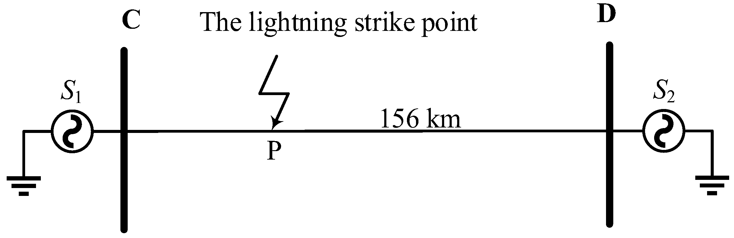
2.1. 220 kV Overhead Line Model

A specific 220 kV overhead line encounters a lightning fault, spanning a total length of 156 km and comprising 480 towers, with an average spacing of 325 m between them. The simulation model is depicted in Figure 1. In Figure 1, ‘C’ represents the left system busbar, and ‘D’ represents the right system busbar. The system employs a Phase model, encountering a lightning fault at a distance C from the 50 km end busbar, with dual lightning lines installed along the line. The power supply voltage is 1.05 times the rated voltage, the value is 230 kV, the system sampling frequency is 1 MHz, and the simulation step is 0.02 μs. The system parameters are shown in Table A1 in Appendix A.

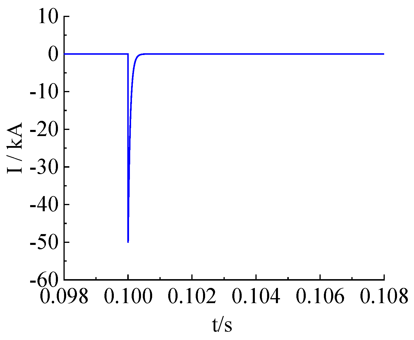
2.2. Lightning Current Model
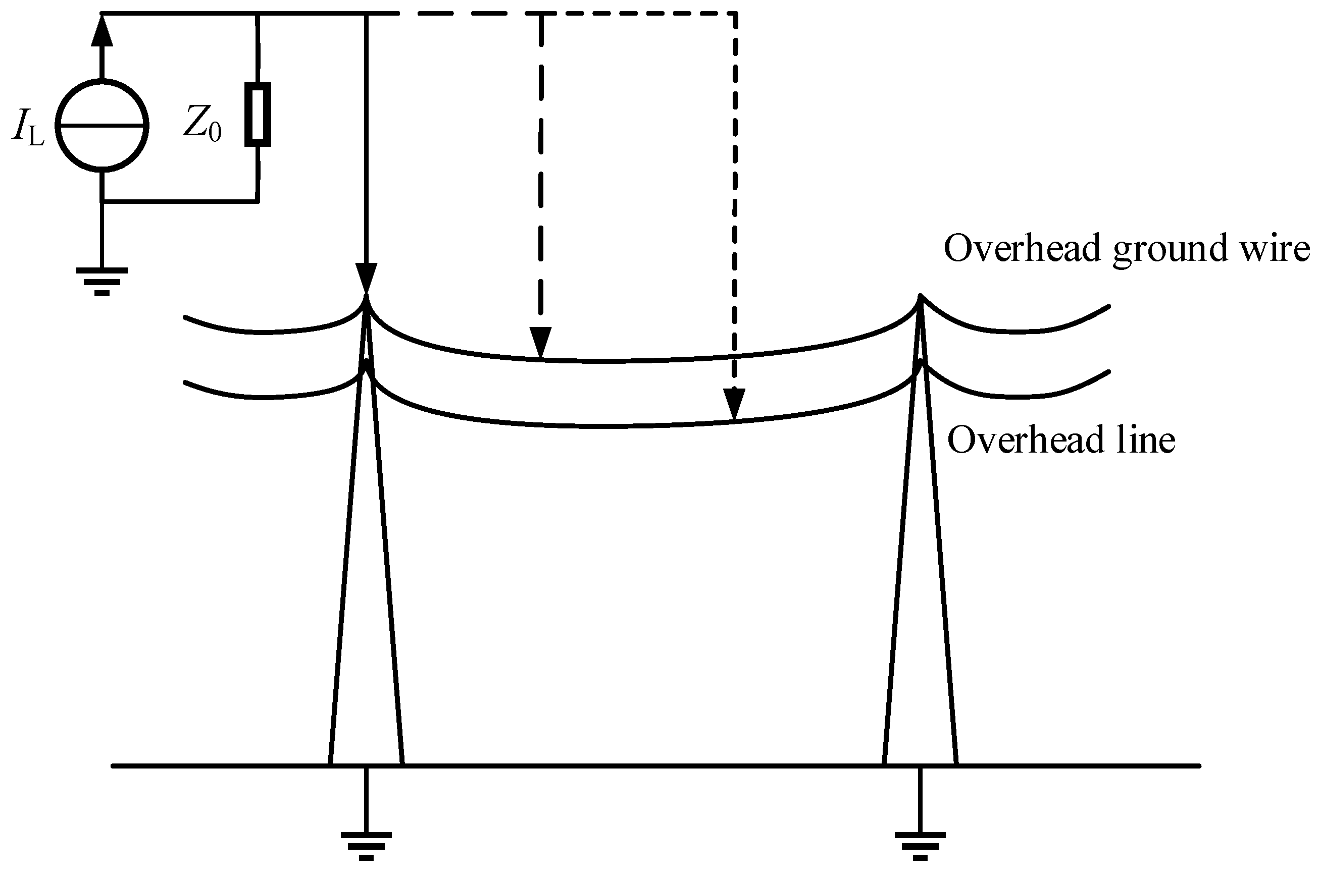
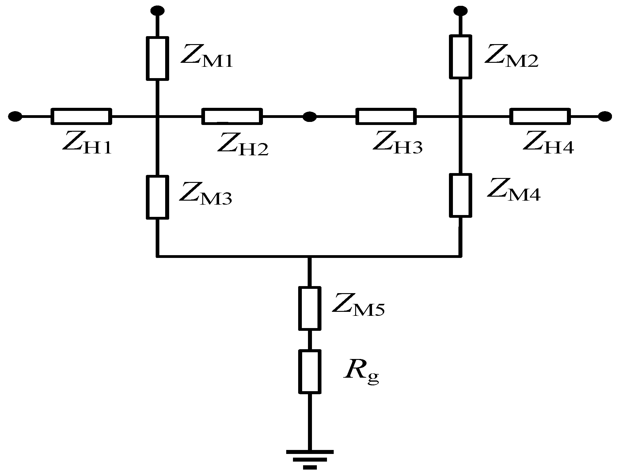
The empirical data indicate that a substantial proportion, ranging from 70% to 90%, of natural lightning carries a negative charge. Therefore, a 1.2/50 μs negative polarity double exponential lightning current model is employed for analysis [16]. Equation (1) represents the calculation for the lightning current, while its waveform is illustrated in Figure 2.
i ( t ) = A I 0 ( e β t e δ t )
In Equation (1), A is the lightning current amplitude correction factor; I0 is the maximum value of the lightning current; and β and δ are the corresponding waveform decay coefficients.
Figure 3 illustrates overhead lines experiencing winding strikes and counterstrikes. In this representation, IL denotes a controlled current source, while Z0 denotes the lightning channel’s equivalent wave impedance, which is specified as 300 Ω [17].

2.3. Tower Model

Various simulation models for transmission towers are commonly used, including the standard model, inductive model, and wave impedance model. The standard model does not account for the phenomenon of overvoltage change, while the inductive model overlooks the influence of the tower on the lightning current wave [18]. This study employs a multi-wave impedance model derived from Bergeron to replicate the behavior of 220 kV cup-type iron towers. The model accurately reproduces the refraction and reflection of lightning current waves on the tower, as depicted in Figure 4. In this context, ZH denotes the transverse carrier wave impedance, ZM denotes the main brace wave impedance of the tower, and Rg represents the grounding resistance.

2.4. Insulator Flashover Model

To minimize the disparity between the simulation outcomes and real-world scenarios, the intersection method (involving the intersection of the overvoltage waveform curve with the volt-second characteristic curve) is selected for the characterization of the insulator flashover. A capacitor paralleled with a voltage-controlled switch is used to simulate the flashover process [19], as depicted in Equation (2):
u ( t ) = 400 L X + 710 L X t 0.75
In Equation (2), LX represents the length of the insulator string.

2.5. Simulation Model Verification
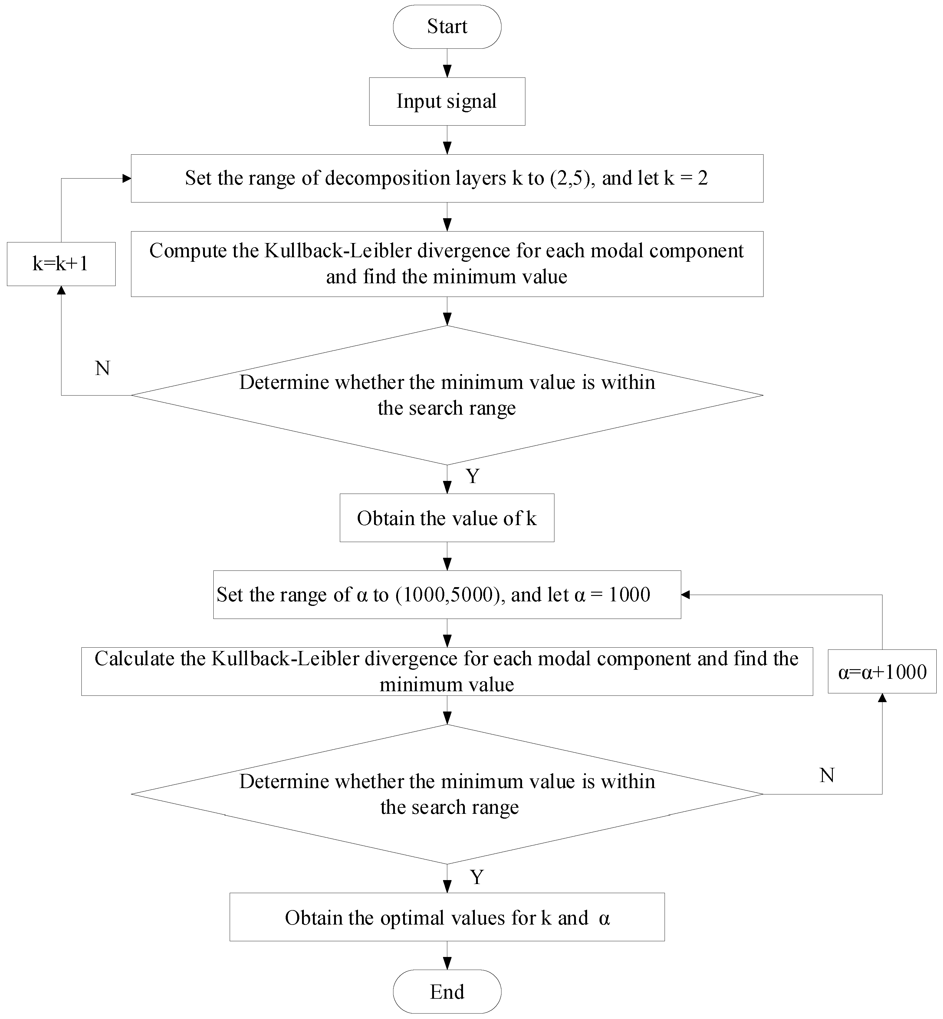
Regulatory standards are used to determine the withstand capability against winding strokes and counterstrike, with the formulas given as Equations (4) and (5).
U 50 % = 533 L X + 132
I 1 = U 50 % / 100
I 2 = U 50 % ( 1 k ) β R g + h a h t k β L t 2.6 + 1 h g h c k 0 h c 2.6
In Equation (5), k 0 is the coupling coefficient.
According to the regulatory standards, the withstand capability against winding strokes is determined to be 12 kA, while the withstand capability against back flashover is found to be 75 kA. The lightning current is conducted at intervals of 0.5 kA, observing whether flashovers occur on the insulator. The simulation results indicate that the withstand capability against winding strokes is 12.5 kA, while the withstand capability against back flashover is 77.5 kA. It complies with the regulatory standards, and the simulated three-phase voltage waveform characteristics, including polarity, amplitude, and shape, align with the descriptions of the fault waveforms in references [20,21]. Therefore, this validates the accuracy of the simulations conducted in this study.

3. VMD Algorithm

The parameters for VMD are frequently established using empirical values or the center frequency observation method. KL divergence is capable of indicating the similarity between two signals, and is therefore employed as the objective function for optimizing the VMD algorithm. In accordance with modulation standards, IMFs are characterized as amplitude-frequency modulated signals, as depicted in Equation (6):
u k ( t ) = A k ( t ) c o s [ φ k ( t ) ]
In Equation (6), φk(t) is the phase function and Ak(t) is the instantaneous amplitude.
The original signal is decomposed into k intrinsic mode components known as Intrinsic Mode Functions (IMFs), along with the amplitude uk(t) and center frequency ωk(t) of each IMF. The bandwidth of each modal signal is estimated through the application of Gaussian smoothness [22], and the constraint problem is expressed as follows:
m i n { u k } , { ω k } { k | | t [ ( δ ( t ) + j / π t ) × u k ( t ) ] e j ω k t | | 2 2 } s . t . k u k = f
In Equation (7), {uk} are the k decomposed modal components of the signal and {ωk} are the central frequencies of each component.
To determine the optimal solution for constrained variational mode mingling, a quadratic penalty factor α and Lagrange multipliers λ are introduced, leading to the equation of an augmented Lagrangian function [23] as follows:
L ( { u k } , { ω k } , λ ) = | | f ( t ) k u k ( t ) | | 2 2 + < λ ( t ) , f ( t ) k u k ( t ) > + α k | | t [ ( δ ( t ) + j / π t ) u k ( t ) ] e j ω k t | | 2 2
In Equation (8), * is the convolution operator. The Alternation Direction Method of Multipliers (ADMM) is a technique that involves iteratively updating {uk} and {ωk} in order to seek the Lagrange saddle point, until the iteration termination criteria are satisfied. This process is expressed as follows:
u k n + 1 = | | f ( t ) k u k ( t ) + λ ( t ) / 2 | | 2 2 + a r g m i n u k X { α | | t [ ( δ ( t ) + j / π t ) × u k ( t ) ] e j ω k t | | 2 2 }
ω k n + 1 = a r g m i n ω k X { | | t [ ( δ ( t ) + j / π t ) × u k ( t ) ] e j ω k t | | 2 2 }
KL divergence, also referred to as relative entropy, quantifies the difference between two probability distributions P and Q [24]. It is defined in Equation (11):
D K L ( P | | Q ) = i P ( i ) log P ( i ) Q ( i )
The probability density distribution of a signal is determined by applying the kernel density estimation method to the probability distribution and probability density distribution functions of two signals, as depicted in Equation (12):
P ( x ) = 1 n h i = 1 n k x i x h , x R
k ( u ) = 1 2 π e u 2 / 2
In Equation (12), P(x) is the probability density function and h is the window parameter, also referred to as the smoothing parameter. Equation (13) defines the Gaussian kernel function. The process by which KL divergence enhances the performance of VMD is depicted in Figure 5.

4. PE Algorithm

4.1. Introduction to PE

PE was introduced by Bandt et al. [25] as a technique for identifying randomness and dynamical variations in time series data. Principal Component Analysis (PCA) is recognized for its simplicity, rapid computational speed, and robust resistance to interference, rendering it especially well-suited for nonlinear data. The computational method can be outlined in Equation (11).
Upon conducting phase space reconstruction [26], the time series {x(i), i = 1, 2, ..., N} of length N transforms into the following time series:
X ( 1 ) = { x ( 1 ) , x ( 1 + λ ) , , x ( 1 + ( m 1 ) λ ) } X ( k ) = { x ( i ) , x ( i + λ ) , , x ( i + ( m 1 ) λ ) } X ( N ( m 1 ) λ ) = { x ( N ( m 1 ) λ ) , x ( N ( m 2 ) λ ) , , x ( N ) }
In Equation (14), m is the embedding dimension and λ is the time delay.
The m vectors of X(i), denoted as X(i) = {x(i), x(i+λ), ..., x(i+(m−1)λ)}, are rearranged in ascending order as follows:
X ( i ) = { x ( i + ( j 1 1 ) λ ) x ( i + ( j 2 1 ) λ ) x ( i + ( j m 1 ) λ }
If x(i + (ji1 − 1)λ) = x(i + (ji2 − 1)λ) exists, the values are arranged based on the magnitude of j, such that when jk1 < jk2, it implies: x(i + (ja − 1)λ ≤ x(i+(ja − 1)λ).
Therefore, any vector X(i) has the potential to generate a set of symbolic sequences:
S ( g ) = [ j 1 , j 2 , , j m ]
In Equation (16), g = 1, 2, ..., k, km!. The m symbols [j1, j2, ..., jm] amount to m factorial permutations. According to various permutations [27], there are m! corresponding permutations. There are various symbolic sequences, with S(g) representing just one of m!. The probability of occurrence for each type of symbolic sequence is calculated through P 1 , P 2 , , P k , g = 1 k P g = 1 .
The PE of the time series {x(i), i = 1, 2, ..., N} can be expressed in terms of Shannon entropy as follows [28]:
H p ( m ) = g = 1 k P g ln P g
When Pg = 1/m!, the function Hp(m) reaches its maximum value at In(m!). PE Hp(m) can be normalized using the In(m!) transformation. The expression is presented as follows:
H p = H p ( m ) / I n ( m ! )
The range of Hp values falls within the interval 0 ≤ Hp ≤ 1. The magnitude of Hp serves as an indicator of the level of randomness present in the time series. A higher Hp value indicates a greater degree of randomness in the time series, while a lower Hp value suggests a more predictable pattern in the time series.

4.2. Selection of PE Parameters

In the calculation of PE, it is necessary to determine three parameters: the length of the time series N, the embedding dimension m, and the time delay λ. The selection of the embedding dimension, denoted as m, typically falls within the range of 3 to 7. If m is too small, the resulting reconstructed vector will contain an insufficient number of states, thereby undermining the meaningfulness of the algorithm. Conversely, if m is too large, the reconstruction of the phase space will lead to a homogenization of the time series, resulting in increased computational demands and an inability to capture subtle changes in the series. As a result, this paper chooses m = 5. The time delay parameter λ exerts a negligible influence on the calculation of the time series. In this study, a value of λ = 1 is selected.

4.3. Symplectic Geometry Mode Decomposition

4.3.1. Phase Space Reconstruction

According to Takens’ embedding theorem, a one-dimensional discrete original signal s = (x1, x2, ..., xn) [29] can be topologically equivalent to the construction of a multidimensional time series matrix, denoted as the trajectory matrix X in Equation (19):
X = x 1 x 1 + τ x 1 + ( d 1 ) τ x 2 x 2 + τ x 2 + ( d 1 ) τ x m x m + τ x m + ( d 1 ) τ
In Equation (16): d is the difference dimension and τ is the delay time. The trajectory matrix X is characterized by two primary parameters, d and τ. Varied values of d and τ can yield distinct matrices X, thereby exerting a substantial influence on the analytical results.

4.3.2. Symplectic Orthogonal Matrix QR Decomposition

Let A = XT X construct M as a Hamilton matrix [30], namely:
M = A T 0 0 A
Let N = M2, then both M and N be Hamilton matrices. A symplectic orthogonal matrix Q is to be constructed such that:
Q T N Q = B R 0 B T
In Equation (21), B is an upper triangular matrix, bij = 0(i > j + 1). The transformation of N using the defined symplectic orthogonal type for 2 yields B, with eigenvalues λ1, λ2, ..., λd. According to the given properties, σ i = λ i , where Qi represents the eigenvectors of matrix A corresponding to σi. By constructing transformation coefficients S i = Q i T X T using the matrix Qi and the trajectory matrix X, and defining Y = QiSi, the matrix Xi = YT can be obtained. The original matrix X for phase space reconstruction comprises d components, which can be expressed as X = X1 + X2 + ... + Xd.

4.3.3. Diagonal Averaging

This step involves transforming each component Xk (1 ≤ kd) into a time series of length n, resulting in d sets of time series, each with a length equivalent to the original time series n.
Let Xm×d = (xij)m×d, d* = min(m,d), m* = max(m,d), n = m + (d − 1)τ.
y k = 1 k p = 1 k y p , k p + 1 * , 1 k d   1 d p = 1 d * y p , k p + 1 * , d   k m   1 n k + 1 n p = k m * + 1 n m * + 1 y p , k p + 1 * , m   < k n
Equation (22) yields a time series Yk = (y1, y2, ..., yn) based on Xi, leading to d groups of independent superimposed components in the time domain, specifically the d of Symplectic Geometry Component (SGC) components.

4.4. PE Improved SGMD

Initially, an empty array z is initialized. The multiscale PE function is employed for computing the PE of every row in the SGC matrix, and the outcomes are saved in array z. Subsequently, the values in array z are sorted, and the resulting sorted indices are retained. The minimum and maximum values in array z are calculated and then assigned to d1 and d2, respectively. The value of d is determined by the equation d = (d2d1)/4. Four arrays, namely s1, s2, s3, and s4, are initialized and populated based on the conditions associated with the value of z. These arrays store the sums of rows of the SGC matrix. As z values are iterated through, the corresponding rows of SGC are added to the respective s arrays based on the specified conditions. The arrays are stacked vertically and transposed to derive the x array, which is subsequently assigned to the output variable.

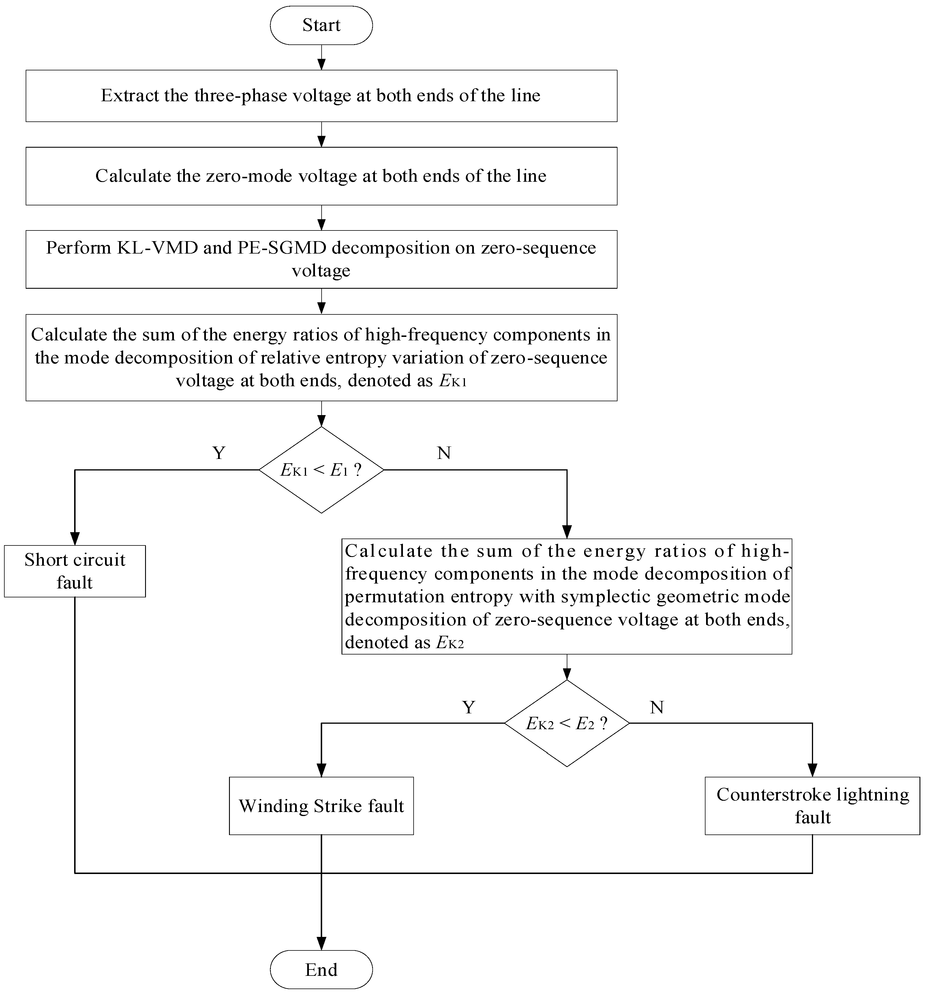
5. Method for Identifying Lightning Faults

5.1. Identification of Short-Circuit and Direct Strike Faults

The study primarily focuses on direct strikes as induced lightning poses minimal threat to 220 kV overhead lines. Utilizing PSCAD v5.0.2 software for simulating the model depicted in Figure 1, single-phase short-circuit, winding strike, and counterstrike faults are configured to take place at a distance of 50 km from the C end of the line. The voltage traveling waves in three phases, measured at the C end, are depicted in Figure 6:
The simulated waveforms were observed, and the following differences were illustrated as follows:
(1)
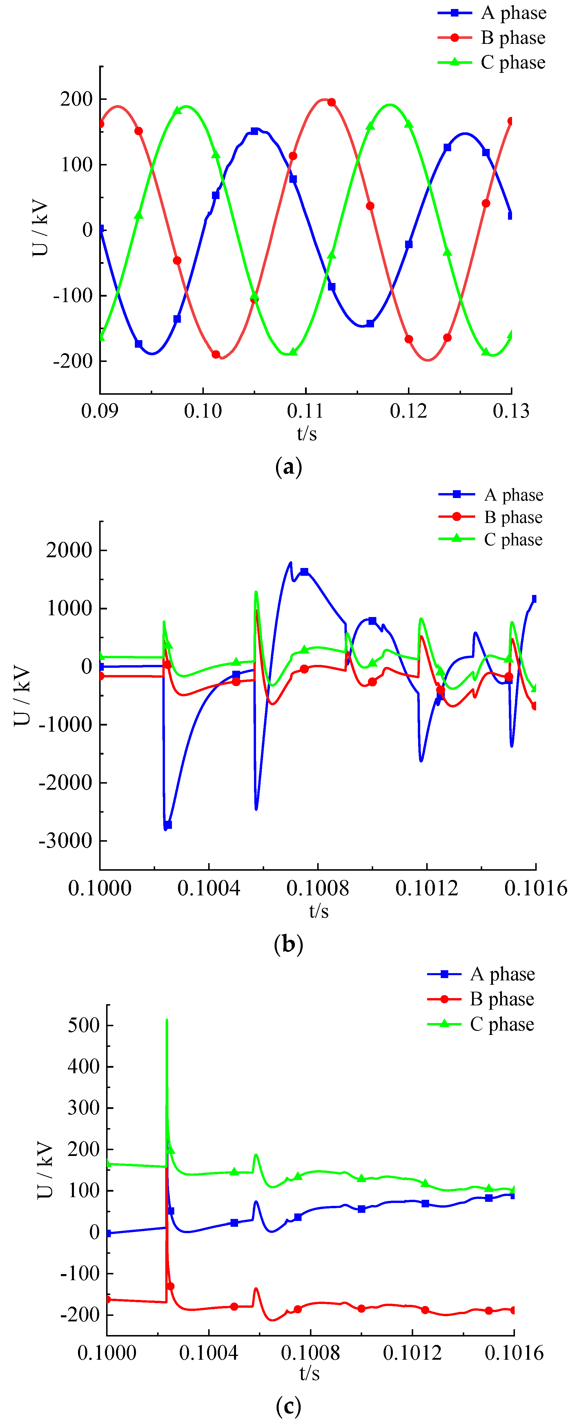
As depicted in Figure 6a, in the event of a single-phase ground short circuit experienced by phase A, its voltage amplitude is lower than that of phases B and C, with a difference of approximately 100 kV. The voltage value of the short-circuit process fluctuates in accordance with a sine function.
(1)
In Figure 6b,c, the voltage amplitude of winding strike faults exceeds that of counterstrike faults for the lightning current in Figure 2. Specifically, the first wavefront voltage amplitudes reach approximately 2800 kV and 500 kV, respectively, and both exhibit steep shapes. When lightning bypasses lightning rods and poles and directly strikes the phase A conductor, the polarity of its voltage traveling wave is opposite to that of the other two phases. When the lightning rod or pole is directly struck by lightning, the transient voltage traveling wave polarities of all three phases are identical.
The conclusions drawn are based on the comparison of time-domain waveforms, and it is important to acknowledge that there are inherent limitations in practical applications. For instance, variations in fault distances may potentially affect the accuracy of identification results. This paper examines the transient energy ratio of high-frequency components of zero-mode voltage from a theoretical standpoint, and subsequently proposes a more comprehensive method for identification.
The electromagnetic coupling among the three-phase transmission lines necessitates the use of Karhunen–Loeve phase-mode transformation to mitigate its impact [31], as demonstrated in Equation (23).
U 0 U 1 U 2 = 1 3 1 1 1 1 1 0 1 0 1 U a U b U c
In Equation (23), U0, U1, and U2 denote the zero-mode component, line mode 1 component, and line mode 2 component of the phase voltages Ua, Ub, and Uc, respectively, as per Karhunen–Loeve transformation.
When the lightning strike occurs near the C end, there is a high detected transient energy ratio of the high-frequency component. Conversely, when the lightning strike is near the D end, the detected transient energy ratio of the high-frequency component is low, and vice versa. In light of the unpredictable characteristics of lightning strikes on overhead lines, calculating the combined energy ratios from both ends is necessary to mitigate the influence of the strike distance on the transient energy ratio of high-frequency components. The zero-mode voltage at both ends of the line is extracted and then subjected to KL-VMD decomposition, as depicted in Figure 7. In Figure 7, IMF1 represents the first intrinsic mode component of zero-mode voltage decomposed by KL-VMD; IMF2 represents the second intrinsic mode component of zero-mode voltage decomposed by KL-VMD; IMF3, IMF4, and so on.
Through optimization, the m intrinsic mode components are decomposed at the D end, while the n intrinsic mode components are decomposed at the C end. The absolute values are computed to derive the energy distribution of the IMF (I1, I2, ..., Im and F1, F2, ..., Fn), extracting the high-frequency components of the highest layer Im and Fn.
The calculation involves determining the sum of the transient energy ratios of the high-frequency components of the zero-mode voltage relative entropy at both ends of the line, denoted as EK1. The definition is as follows:
E K 1 = I m i = 1 m I i + F n i = 1 n F i
In Equation (24), m and n are the number of KL-VMD decomposed components IMF at the C and D ends, respectively, and i is the starting index.
Table 1 presents the summation of the energy ratios of the high-frequency components of the relative entropy of the zero-mode voltage at both ends of the line, denoted as EK1, for short-circuit, winding strike, and counterstrike faults at varying distances from the C end. The data presented in Table 1 indicate that the EK1 value for lightning faults significantly exceeds that for single-phase ground short circuits. Consequently, a threshold of E1 = 0.001 is established. If E1 > EK1, it corresponds to a short-circuit fault; if E1 is less than or equal to EK1, it corresponds to a direct strike fault. The lightning current functions as a unipolar high-frequency impulse signal, whereas a short-circuit fault can be likened to the application of a reverse voltage source. Consequently, the EK1 value for short-circuit faults is lower. Extensive simulation data calculations demonstrate that the method is capable of accurately identifying short-circuit faults, but it does not differentiate between winding strike and counterstrike faults.

5.2. Identification of Winding Strike and Counterstrike Faults

To accurately differentiate between winding and counterstrike faults, it is essential to employ a suitable method that effectively identifies the transient differences between the two. The SGMD method demonstrates proficiency in signal decomposition by addressing the challenge of empirical parameter selection in EEMD methods and wavelet transforms, as well as circumventing the issue of forced component in LCD methods. Consequently, it achieves enhanced accuracy in fault identification.
At the outset, the zero-mode voltage at both terminals of the line is decomposed using PE-SGMD, with the objective of optimizing the decomposition into p intrinsic mode components at the C terminal and q intrinsic mode components at the D terminal. The absolute values are computed to derive the energy distribution of the IMF (M1, M2, ..., Mp and W1, W2, ..., Wq) by extracting the high-frequency components Mp and Wq from the highest layer. Finally, the calculation involves determining the sample entropy, symplectic geometry mode decomposition, and the high-frequency component energy ratio EK2 of the zero-mode voltage at both ends of the line, which is defined as follows:
E K 2 = M p i = 1 p M i + W q i = 1 q W i
In Equation (25), p and q are the numbers of PE-SGMD decomposed components IMF at the C and D ends, respectively, and i is the starting index.
The data presented in Table 2 indicate disparities in the EK2 values between winding strike faults and counterstrike faults. The EK2 values for winding strike faults are consistently below 0.08, whereas the EK2 values for counterstrike faults consistently exceed 0.08. Consequently, a threshold of EK2 = 0.08 has been established for differentiation. The flowchart illustrating the lightning fault identification criterion can be observed in Figure 8.

6. Simulation Validation

Utilizing the overhead line model depicted in Figure 1, simulations are performed for various operational conditions, such as short-circuit, winding strike, and counterstrike faults. The double exponential model for the lightning current is standardized with a 1.2/50 μs and 2.6/50 μs waveform, with initial phase angles set at 0° and 90°. The amplitude range of the winding lightning current is set between 30 and 70 kA, while the counterstrike lightning current amplitude range is set between 50 and 90 kA. The symmetrical line configuration places the lightning fault point P at a distance of 2080 km from the busbar. The fault range for the single-phase ground short circuit and two-phase ground short circuit is set between 2070 km. Transition resistances are established at 10 Ω, 30 Ω, 50 Ω, 70 Ω, and 100 Ω, resulting in a total of 300 sample data sets. The data are imported into MATLAB for identification, and certain calculation results are presented in Table 3.
The analysis of the data suggests that the method yields high recognition results for short-circuit, winding strike, and counterstrike faults across various operating conditions. The use of KL-VMD and SE-SGMD for extracting high-frequency components, in combination with specific criteria, has been shown to facilitate the efficient and accurate identification of overhead line fault types in diverse scenarios.
Selecting different lightning current amplitudes, distances, and initial phase angles, 30 sets each for winding strike faults and counterstrike faults were chosen. The results were compared with the methods in references [32,33], as shown in Table 4. it can be observed that the recognition accuracy of the method proposed in this paper is higher than the other two methods in all cases. This also validates the effectiveness of the criteria used.

7. Conclusions

This study has developed a model for identifying overhead line lightning faults by employing KL-VMD and SE-SGMD to decompose the zero-mode voltage. The study also established lightning recognition criteria through extensive data calculations, resulting in the following conclusions:
(1)
In situations where signal decomposition is hindered by challenges such as modal mingling, the utilization of KL-VMD can automatically optimize the decomposition layers and penalty factors. This approach effectively extracts transient characteristic quantities, demonstrating its strong adaptability in fault signal decomposition;
(2)
A criterion is proposed for identifying winding strike, counterstrike, and short-circuit faults by analyzing the fault stage traveling wave amplitude, wavefront polarity, rate of change, along with the modal energy distribution using KL-VMD and PE-SGMD. Following thorough data calculations, the validity and accuracy of this criterion have been confirmed;
(3)
The criterion demonstrates high reliability in accurately distinguishing between short-circuit faults and lightning conditions under various lightning current amplitudes, distances, and initial phase angles. It also provides a reference for line fault identification.

Author Contributions

Conceptualization, X.D.; methodology, X.D.; software, J.L.; validation, Z.D.; formal analysis, X.D.; writing—original draft preparation, X.D. and J.L.; writing—review and editing, S.H.; visualization, M.C.; supervision, L.H. All authors have read and agreed to the published version of the manuscript.

Funding

This research was funded by the key laboratory of the Xinjiang Uygur Autonomous Region open for research projects (2023D04029), the key research and development program projects in the Xinjiang Uygur Autonomous Region (2022B01003-3), and the graduate innovation projects in the Xinjiang Uygur Autonomous Region (XJ2023G051).

Data Availability Statement

Data are contained within the article.

Conflicts of Interest

Author Xinsheng Dong was employed by the company Xinjiang Electric Power Research Institute, State Grid Xinjiang Electric Power Co., Ltd. Author Zhongkai Dong was employed by Turpan Power Supply Company, State Grid Xinjiang Electric Power Co., Ltd. Author Minbo Cai was employed by Altay Power Supply Company, State Grid Xinjiang Electric Power Co., Ltd. The remaining authors declare that the research was conducted in the absence of any commercial or financial relationships that could be construed as a potential conflict of interest.

Appendix A

Table A1. The system parameters.
System ParametersNumeric Value
power supply voltage230 kV
sampling frequency1 MHZ
simulation time step0.02 μs
rise time1.2 μs
half-value time50 μs
lightning channel impedance300 Ω
total length of the circuit156 km
ground resistance10 Ω

References

  1. Dong, X.; Zhang, D. Across the Tianshan mountains of 750 kV transmission line lightning risk assessment. Electr. Power Sci. Eng. 2015, 31, 66–71. [Google Scholar]
  2. Zhang, D.; Dong, X.; Tao, F.; Wang, S. Research on reduction of the monsoon influence on the transmission line shielding failure. Insul. Surge Arresters 2014, 259, 57–61. [Google Scholar]
  3. Zhao, C.; Chen, J.; Gu, S.; Ruan, J.; Li, X.; Tong, X.; Hu, W. Research on differentiated lightning protection comprehensive management for the 500-kV power network in the area near the three gorges project. IEEE Trans. Power Deliv. 2011, 27, 337–352. [Google Scholar]
  4. Jiang, K.; Du, L.; Chen, H.; Yang, F.; Wang, Y. Non-contact measurement and polarity discrimination-based identification method for direct lightning strokes. Energies 2019, 596, 263. [Google Scholar] [CrossRef]
  5. Zou, G.; Gao, H.; Zhu, F.; Wang, H. Integral identification method of lightning stroke and fault for transmission line. Power Syst. Prot. Control 2012, 40, 43–48. [Google Scholar]
  6. Shu, H.; Wang, Y.; Cheng, C.; Sun, S. Analysis of electromagnetic transient and fault detection on ±800 kV UHVDC transmission lines under lightning stroke. Proc. CSEE 2008, 28, 93–100. [Google Scholar]
  7. Sima, W.; Xie, B.; Yang, Q.; Wang, J. Identification of lightning over-voltage about UHV transmission line. High Volt. Eng. 2010, 36, 306–312. [Google Scholar]
  8. Guo, N.; Qin, J. Locating method of short-circuit point for transmission lines under lightning stroke fault. Autom. Electr. Power Syst. 2009, 33, 74–77+85. [Google Scholar]
  9. Zhong, H.; Chen, J.; Fu, Q.; Hua, M. Lightning strike identification algorithm of an all-parallel auto-transformer traction power supply system based on morphological fractal theory. IEEE Trans. Power Deliv. 2023, 38, 2119–2132. [Google Scholar] [CrossRef]
  10. Si, D.; Shu, H.; Chen, X.; Yu, J. Study on characteristics and identification of transients on transmission lines caused by lightning stroke. Proc. CSEE 2005, 25, 64–69. [Google Scholar]
  11. Gao, Y.; Zhu, Y.; Yan, H.; Yan, H. Identification of lightning strike and short-circuit fault based on wavelet energy spectrum and transient waveform characteristics. Mechatron. Ind. Inform. 2014, 596, 713–718. [Google Scholar] [CrossRef]
  12. Chen, Z.; Pei, H.; Teng, C. Identification of transmission line lightning based on HHT. Int. J. Smart Home 2016, 10, 201–212. [Google Scholar]
  13. Zhao, H.; Wang, X.; Gao, C. Traveling wave fault location method for high voltage transmission lines based on FIMD and Hilbert transform. Electr. Meas. Instrum. 2020, 57, 77–82. [Google Scholar]
  14. Han, Z.; Rao, S.; Jiang, Y.; Wang, S.; Liu, J.; Lu, Y. Energy ratio function-based traveling-wave fault location for transmission lines. Power Syst. Technol. 2011, 35, 216–220. [Google Scholar]
  15. Liu, J.; Su, Y.; Deng, R.; Sun, F. Performance degradation assessment of rolling bearing based on KL-VMD and comprehensive characteristic indexes. J. Electron. Meas. Instrum. 2022, 36, 78–88. [Google Scholar]
  16. Xi, Y.; Cui, Y.; Tang, X.; Li, Z.; Zeng, X. Fault location of lightning strikes using residual analysis based on an adaptive kalman filter. IEEE Access 2019, 7, 88126–88137. [Google Scholar] [CrossRef]
  17. Gu, Y.; Song, G.; Guo, A.; Tao, R.; Liu, Y. A lightning recognition method for DC line travling-wave protection of HVDC. Proc. CSEE 2018, 38, 3837–3845+4024. [Google Scholar]
  18. Long, Y.; Yao, C.; Mi, Y.; Hu, D.; Yang, N.; Liao, Y. Identification of direct lightning strike faults based on mahalanobis distance and S-transform. IEEE Trans. Dielectr. Electr. Insul. 2015, 22, 2019–2030. [Google Scholar] [CrossRef]
  19. Song, X.; Gao, Y.; Ding, G.; Yan, H. Lightning strike interference and fault identification of transmission system. Insul. Surge Arresters 2021, 299, 96–102+110. [Google Scholar]
  20. Gao, Y. Study on Method of Lightning Strike Identification and Fault Location of Transmission Lines Based on Current Traveling Waves. Ph.D. Thesis, North China Electric Power University, Baoding, China, 2016. [Google Scholar]
  21. Liang, Z. Study on the Simulation and Identification of Lightning Strike on Transmission Line. Master’s Thesis, North China Electric Power University, Baoding, China, 2014. [Google Scholar]
  22. Deng, L.; Zhang, A.; Zhao, R. Intelligent identification of incipient rolling bearing faults based on VMD and PCA-SVM. Adv. Mech. Eng. 2022, 14, 1–18. [Google Scholar] [CrossRef]
  23. Li, J.; Zhu, X.; Guo, J. Bridge modal identification based on successive variational mode decomposition using a moving test vehicle. Adv. Struct. Eng. 2022, 25, 2284–2300. [Google Scholar] [CrossRef]
  24. Harmouche, J.; Delpha, C.; Diallo, D. Incipient fault amplitude estimation using KL divergence with a probabilistic approach. Signal Process. 2016, 120, 1–7. [Google Scholar] [CrossRef]
  25. Bandt, C.; Pompe, B. Permutation entropy: A natural complexity measure for time series. Phys. Rev. Lett. 2002, 88, 174102. [Google Scholar] [CrossRef]
  26. Li, X.; Ouyang, G.; Richards, D.A. Predictability analysis of absence seizures with permutation entropy. Epilepsy Res. 2007, 77, 70–74. [Google Scholar] [CrossRef]
  27. Ricci, L.; Politi, A. Permutation entropy of weakly noise-affected signals. Entropy 2022, 24, 54. [Google Scholar] [CrossRef]
  28. Ouyang, G.; Li, J.; Liu, X.; Li, X. Dynamic characteristics of absence EEG recordings with multiscale permutation entropy analysis. Epilepsy Res. 2013, 104, 246–252. [Google Scholar] [CrossRef]
  29. Zheng, Z.; Xin, G. Fault feature extraction of hydraulic pumps based on symplectic geometry mode decomposition and power spectral entropy. Entropy 2019, 21, 476. [Google Scholar] [CrossRef]
  30. Pan, H.; Yang, Y.; Li, X.; Zheng, J.; Cheng, J. Symplectic geometry mode decomposition and its application to rotating machinery compound fault diagnosis. Mech. Syst. Signal Process. 2019, 114, 189–211. [Google Scholar] [CrossRef]
  31. Dai, J.; Liu, Y.; Jiang, W.; Liu, Z.; Sheng, G.; Yan, Y.; Jiang, X. Identification of back striking and shielding failure on transmission line based on time domain characteristics of traveling wave. Trans. China Electrotech. Soc. 2016, 31, 242–250. [Google Scholar]
  32. Li, J. Research on the Identification of Direct Lightning Overvoltage on 110 kV Transmission Line. Master’s Thesis, Hefei University of Technology, Hefei, China, 2021. [Google Scholar]
  33. Liu, Y.; Zhu, T.; Geng, Y.; Cheng, D.; Yan, B.; Cao, S.; Fang, D. Lightning tripping fault type identification method based on multi-scale generalized S-transform and deep residual network. Insul. Surge Arresters 2021, 304, 94–101. [Google Scholar]
Figure 1. Simulation system model.
Processes 12 00329 g001
Figure 2. Lightning current waveform.
Processes 12 00329 g002
Figure 3. Schematic diagram of lightning-struck line.
Processes 12 00329 g003
Figure 4. Multi-wave impedance model of tower.
Processes 12 00329 g004
Figure 5. KL divergence optimized VMD parameter flowchart.
Processes 12 00329 g005
Figure 6. Three-phase voltage waveform during faults: (a) short-circuit fault; (b) winding strike fault; (c) counterstrike fault.
Processes 12 00329 g006
Figure 7. KL-VMD decomposition results.
Processes 12 00329 g007
Figure 8. Fault type identification process using criterion method.
Processes 12 00329 g008
Table 1. Summation of the energy ratio of high-frequency components of relative entropy in zero mode-voltage at both ends of the line under different conditions EK1.
Fault TypePC/kmPD/kmEK1
Short-Circuit Fault301261.3326 × 10−5
Short-Circuit Fault401161.3516 × 10−5
Short-Circuit Fault501061.4201 × 10−5
Short-Circuit Fault60961.5051 × 10−5
Winding Strike301260.0159
Winding Strike401160.0356
Winding Strike501060.5490
Winding Strike60960.2999
Counterstrike301260.1838
Counterstrike401160.1629
Counterstrike501060.1717
Counterstrike60960.1789
Table 2. Summation of the energy ratio of the high-frequency component in PE symplectic geometric modal component of zero-mode voltage at both ends of the line under different conditions Ek2.
Fault TypePC/kmPD/kmEk2
Winding Strike301260.0026
Winding Strike401160.0043
Winding Strike501060.0033
Winding Strike60960.0029
Winding Strike70860.0068
Counterstrike301260.8985
Counterstrike401160.9310
Counterstrike501060.6551
Counterstrike60960.8733
Counterstrike70860.4693
Table 3. Partial calculation results.
Distance/km30 km50 km70 km
EK1EK2ResultEK1EK2ResultEK1EK2Result
Phase A ground short circuit, Rg = 30 Ω, θ = 90°1.3326 × 10⁻⁵Short Circuit1.4201 × 10−5Short Circuit2.0681 × 10−5Short Circuit
Phase A ground short circuit, Rg = 50 Ω, θ = 0°1.6745 × 10⁻⁵Short Circuit1.8363 × 10−5Short Circuit2.7329 × 10−5Short Circuit
Phase AB ground short circuit, Rg = 30 Ω, θ = 90°2.9690 × 10⁻⁵Short Circuit2.6474 × 10−5Short Circuit3.0331 × 10−5Short Circuit
Phase AB ground short circuit, Rg = 50 Ω, θ = 90°3.1702 × 10⁻⁵Short Circuit2.8562 × 10−5Short Circuit3.0805 × 10−5Short Circuit
Winding Strike, Imax = 30 kA,
θ = 0°, 1.2/50 μs
0.31450.0035Winding Strike0.57050.0088Winding Strike0.51660.0088Winding Strike
Winding Strike, Imax = 40 kA,
θ = 0°, 2.6/50 μs
0.31680.0029Winding Strike0.57810.0087Winding Strike0.51960.0091Winding Strike
Winding Strike, Imax = 50 kA,
θ = 90°, 1.2/50 μs
0.01590.0026Winding Strike0.54920.0033Winding Strike0.27930.0068Winding Strike
Winding Strike, Imax = 60 kA,
θ = 90°, 2.6/50 μs
0.01650.0026Winding Strike0.55260.0039Winding Strike0.28170.0063Winding Strike
Counterstrike, Imax = 90 kA,
θ = 0°, 1.2/50 μs
0.19511.1181Counterstrike0.19060.8240Counterstrike0.16450.4694Counterstrike
Counterstrike, Imax = 100 kA,
θ = 90°, 2.6/50 μs
0.17260.5824Counterstrike0.15660.5809Counterstrike0.14550.3876Counterstrike
Counterstrike, Imax = 110 kA,
θ = 90°, 1.2/50 μs
0.18380.8985Counterstrike0.17170.6551Counterstrike0.15130.4693Counterstrike
Counterstrike, Imax = 120 kA,
θ = 0°, 2.6/50 μs
0.17880.5922Counterstrike0.18200.5773Counterstrike0.16070.3888Counterstrike
Table 4. Recognition performance of different methods.
Identification MethodNumber of Test SamplesFault Detection Accuracy
Winding Strike FaultCounterstrike Fault
identification methods in the literature 326090.0%88.3%
identification methods in the literature 336095.0%95.0%
KL-VMD+PE-SGMD6096.6%98.3%
Disclaimer/Publisher’s Note: The statements, opinions and data contained in all publications are solely those of the individual author(s) and contributor(s) and not of MDPI and/or the editor(s). MDPI and/or the editor(s) disclaim responsibility for any injury to people or property resulting from any ideas, methods, instructions or products referred to in the content.

