1. Introduction
Power system reliability assessment is an important part of power system planning, design, and operation management. The evaluation results have significant reference value for power system planning and operation [
1,
2]. However, due to the fact that the equipment reliability parameters used in traditional power system reliability assessments are mostly based on the historical fault statistical records, the data quality is not high, and it is easily affected by human factors, resulting in significant errors in reliability assessment results [
3]. In addition, the complexity of operating conditions in the power system, such as large-scale renewable energy integration and diverse user demands, has increased the difficulty of power system reliability assessments [
4].
At present, power system reliability evaluation algorithms to be applied in engineering can be divided into two categories: a state analysis method and Monte Carlo simulation (MCS) method [
5]. The evaluation process of these two methods is basically the same, usually consisting of three parts: system state selection, system state evaluation, and indicator statistics [
6,
7]. Among them, system state evaluation usually requires performing optimal power Fflow (OPF) on system state samples to determine the minimum load shedding of the system. Although DC OPF models with high computational efficiency are often used, state evaluation is the most time-consuming step in reliability analysis due to the involvement of tens or hundreds of thousands of samples. This significantly increases the computational burden and the quality of state samples directly affects the accuracy of evaluation results. Researchers have proposed a series of improved sampling methods, including state space pruning [
8], importance sampling [
9], Latin hypercube sampling [
10], etc. By generating and selecting representative samples, the number of samples required to obtain specific accuracy reliability evaluation results is reduced, thereby reducing computational complexity and improving computational efficiency. Reference [
11] combines Latin hypercube sampling with importance sampling and proposes an improved Latin hypercube method to improve sampling efficiency. Based on importance sampling, references [
12,
13,
14] introduce the cross-entropy algorithm, which constructs the optimal probability distribution of components by changing the probability of fault states, reduces sample variance fluctuations, and accelerates convergence. In detail, reference [
12] combines cross-entropy with MCS for a reliability evaluation of power generation systems; reference [
13] further simplifies the evaluation process of the method proposed in [
12]. After obtaining the cross-entropy probability distribution parameters, the reliability index is obtained by combining fast Fourier decomposition analysis. Reference [
14] considers transmission lines and applies cross-entropy to evaluate power generation and transmission systems, accelerating the convergence of MCS. For sampling states, the power loss of the system in this state depends on the load demand that has not been met after unit scheduling. The solution of this problem is mainly based on the optimal power flow (OPF) algorithm under nonlinear constraints, and the solving process is time-consuming [
15]. Essentially, if the AC OPF model is used, due to the presence of power flow constraints, the mathematical model has nonlinear and non-convex characteristics, making it difficult to ensure optimality.
On the other hand, the reliability assessment of power systems is essentially solving a series of OPF problems with minimum load shedding as the objective function. OPF establishes a mapping relationship between the system state and optimal operating indicators (such as minimum load shedding), which can be regarded as a special type of nonlinear function. Therefore, in principle, it can be fitted and approximated through data-driven methods. In order to accelerate system state evaluation, researchers have proposed methods such as neural networks [
16,
17], learning vector quantization networks [
18], and support vector machines [
19] to replace the traditional model of linear programming. However, the selection, quantity, and computational accuracy of training samples have not been uniformly solved. Reference [
20] proposed a three-stage OPF solving framework and utilized a stacked extreme learning machines to build the mapping relationships of each stage. In addition, the rapidly developing deep learning technology has injected new vitality into OPF fitting. Reference [
21] used a deep neural network (DNN) to fit the relationship between node injection power, active power difference of each branch before and after branch disconnection, and voltage phase, and approximately solved the DC power flow equation. Reference [
22] used stacked denoising auto encoders to fit the relationships between the electrical and thermal load power of each node, as well as the gas load flow rate with voltage, pressure, pipeline flow rate, etc., achieving a data-driven multi-energy flow calculation. In terms of an OPF solution, similar to power flow analysis, reference [
23] used DNN to learn the mapping relationship between system load distribution and generator power allocation, thereby solving the DC optimal power flow model. Unfortunately, methods represented by support vector machines and conventional neural networks are highly sensitive to the selection of hyperparameters such as learning rate, batch size, network structure, etc. Choosing inappropriate hyperparameters may lead to model training failure or poor performance. Furthermore, due to the complexity and nonlinearity of neural networks, their decision-making process often lacks interpretability. This makes it difficult for power system operators to understand why the model makes a certain decision, making it difficult to effectively debug and optimize it.
In all, there are still some challenges that urgently need to be addressed as follows.
The above methods have made some progress in reducing the calculation time of reliability assessments, but there is still a common limitation: if the reliability parameters of components or network topology change, a new reliability assessment must be conducted to obtain the changed system reliability indicators. In engineering applications that require repeated reliability evaluations, although the application of the above methods can shorten the calculation time of a single reliability evaluation, repeated evaluations still require significant time consumption.
These studies can effectively improve the solving speed of a large number of repetitive OPF calculations, but still face difficulties in feature extraction, overfitting, and difficulty adapting to complex network topology changes, which cannot be directly applied to reliability analysis.
To address the aforementioned issues, this paper proposes a hybrid data-driven approach to achieve a rapid reliability assessment of power systems. The innovation points of this paper can be summarized as follows.
- (1)
The analytical expressions for the reliability indicators and component parameters of the power system are derived. By using this analytical expression, a large number of samples can be quickly obtained under different operating conditions.
- (2)
An online and offline two-stage hybrid data-driven model has been established. Among them, a reliability index regression model based on CNN is constructed, achieving fast solving while ensuring accuracy.
The framework is organized as follows: in
Section 2, the analytical expression between system reliability indicators and component reliability parameters has been derived, which can provide a large number of data samples for offline training quickly. A classification regression CNN model and its detailed design parameters are introduced in
Section 3. Then, the improved IEEE RTS-79 testing system is given to validate the effectiveness and feasibility of the proposed model.
2. Analytical Expression for Reliability Indicators of Power Systems
Sequential Monte Carlo simulation is widely used in the reliability assessment of complex power systems with large-scale renewable energy integration. Currently, there are many commonly used indicators to characterize the reliability of power systems, such as loss of load probability (LOLP), loss of load frequency (LOLF), and expected energy not supplied (EENS), system average interruption frequency index (SAIFI), system average interruption duration index (SAIDI), and so on. In this paper, these three indicators (LOLP, LOLF, and EENS) are highly focused on because SAIFI and SAIDI mainly focus on the frequency and duration of power outages for users, while EENS, LOLF, and LOLP focus more on evaluating whether the power generation capacity of the system can meet the load demand from the perspective of the power system. The reliability assessment in this article focuses more on the overall power generation capacity and margin of the system, rather than the power outage situation of individual users. In addition, other indicators can also be derived from these three indicators. Common component reliability parameters include failure rate λ, repair rate μ and component availability A, etc. This section takes the LOLP, LOLF, and EENS system indicators as examples to introduce the analytical model for power system reliability evaluation. Other models can be obtained using similar methods.
Firstly, the traditional reliability index calculation formulas using the Monte Carlo method are shown in (1)–(3):
Here, represents the total simulation duration; represents the set of all failure times of the system within the total simulation duration; represents the duration of system event s. is a 0–1 variable, if the previous event of system event s does not lose load, ; otherwise ; represents the amount of load shedding for system event s; T is the given duration interval. In this paper, the value of T is set as 8760 h, i.e., one year.
It is assumed that the components involved in the reliability assessment process only have two states of operation and failure, and the faults between each component are independent of each other. For m components, the number of combined states that exist is .
Let
represent the set of system events where
m components are in the
j-th combination state. Therefore, the set of system failure events
in Formulas (1)–(3) can be divided into
M subsets, i.e.,
. Meanwhile, the initial Formulas (1)–(3) can be decomposed into the sum of
M terms, as shown in (4)–(6) below.
Here, taking the LOLP index as an example, the process of establishing a reliability analysis model is derived. Assuming event E indicates a system loss of the load event, events F1–FM represent M combined states corresponding to m components. Obviously, events F1–FM form a complete set of events, with any two events mutually exclusive.
Considering that the faults between each component are independent of each other, combined with the full probability formula, Formula (4) can be rewritten as (7) and (8):
Equation (8) represents the conditional probability of system load loss of event
E occurring when the components are in a combined state
.
depends on the reliability level of (
n −
m) other components under the condition that the system topology, electrical parameters, and operating parameters remain unchanged. Due to the assumption that the reliability parameters of (
n −
m) other components are fixed and unchanging,
is also a fixed and unchanging constant. Due to the independence of faults between components, the calculation formula for
is shown in (9):
Here, and are respectively, the sets of components in working and faulty states in the combined state .
Substituting Formula (9) into Formula (7) yields the analytical expression for the LOLP indicator, which is shown as Formula (10):
Similarly, the analytical expressions for LOLF and EENS indicators are shown in Equations (11) and (12):
Here, the coefficients
in Equation (11) can be calculated based on Equations (13)–(15):
Here,
represents the duration of the system state
s under specific conditions, and
represents the repair rate of component
h. The coefficients in Equation (12) can be calculated based on Equation (16):
Formulas (10)–(12) provide the calculation expression for reliability indicators. When the coefficients in the analytical expression are calculated, time-consuming calculations can be avoided. By simply inputting the reliability parameters of the components into the model, relevant reliability indicators can be obtained. However, the topology, electrical parameters, and operating parameters of the power system often change, which leads to the need to repeatedly calculate the coefficients in the analytical expressions, which to some extent increases the computational burden and makes real-time online fast solving difficult. Therefore, this article adopts a hybrid data-driven strategy, dividing the rapid reliability assessment of the power system into two steps. The first step is to generate a large number of data samples (including system operating parameters and reliability indicators) using analytical expressions. Then, a convolutional neural network (CNN) is trained to quickly obtain the system reliability index under changing operating conditions through CNN.
3. Reliability Index Regression Model of Power System Based on CNN
3.1. Introduction to CNN Model
To ensure that the reliability index calculation results meet the accuracy requirements, it is usually necessary to simulate the operation of the system for millions of hours and evaluate the operation status of tens of thousands of systems. As the scale of renewable energy power increases, the number and degree of uncertainty sources in the system continue to increase, and the number of samples required to cover system operation scenarios will also significantly increase, and the amount of Monte Carlo simulation calculations will also significantly increase. Based on the reliability evaluation analytical model in the previous section, a dataset of reliability indicators under fixed operating conditions can be obtained. Changing the operating conditions of the system to obtain different data samples, providing sufficient data samples for the CNN model is covered in this section.
The calculation of reliability indicators establishes the mapping relationship between system operation status and reliability indicators, which is a key link in reliability evaluation. This section uses a CNN to fit the above mapping relationship and establish a regression model for system reliability indicators, thereby accelerating the process of reliability evaluation.
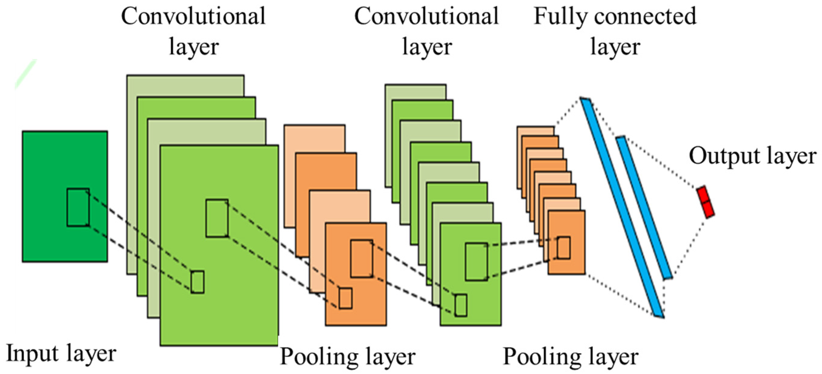
The basic structure of a CNN is shown in
Figure 1, which mainly consists of convolutional layers, pooling layers, and fully connected layers, which can be represented by Equations (17)–(19).
where
X represents the input vector of the convolutional layer;
represents the weight matrix of the
l-th convolutional kernel;
represents the bias term;
f represents the activation function;
represents the
l-th output vector;
p represents the pooling operation, such as taking the maximum value, etc.;
represents the matrix vector for the
l-th pooling surface;
represents a bias term.
3.2. Input Feature Matrix Construction
When using a CNN to fit system reliability indicators, it is necessary to consider the working status of each component and its impact on system operation constraints, such as the impact of generator shutdown on its output range and line shutdown on power flow distribution. At the same time, considering the current construction of new power systems, that is, under the high proportion of renewable energy integration, the uncertainty characteristics of the power system are significant, and the fluctuation range of the system operation status is large. Therefore, this article constructs a CNN input feature matrix as shown in Equation (20).
In the Formula (20), represents the load power of node i; represents the power of renewable energy at node i; represents the power generation capacity of conventional units at node i; represents the self-impedance of node i.
In matrix X, PDi and PRi reflect the time-varying characteristics of node load and renewable energy, reflects the information of generator operation status, and can reflect topological information such as transmission line operation status. When a specific generator or transmission line is forced to shut down, the characteristic parameters and (the first and last nodes of the i line) will change accordingly. In this paper, line losses are not taken into account because in the process of reliability assessment, in order to save calculation time, the DC power flow model is commonly used. The DC power flow model ignores line losses.
Although the number of lines, conventional units, and renewable power stations in the system varies, the input of the different dimensions mentioned above can be unified into a feature matrix that is only related to the number of system nodes n through the processing of Equation (20), for subsequent training and processing.
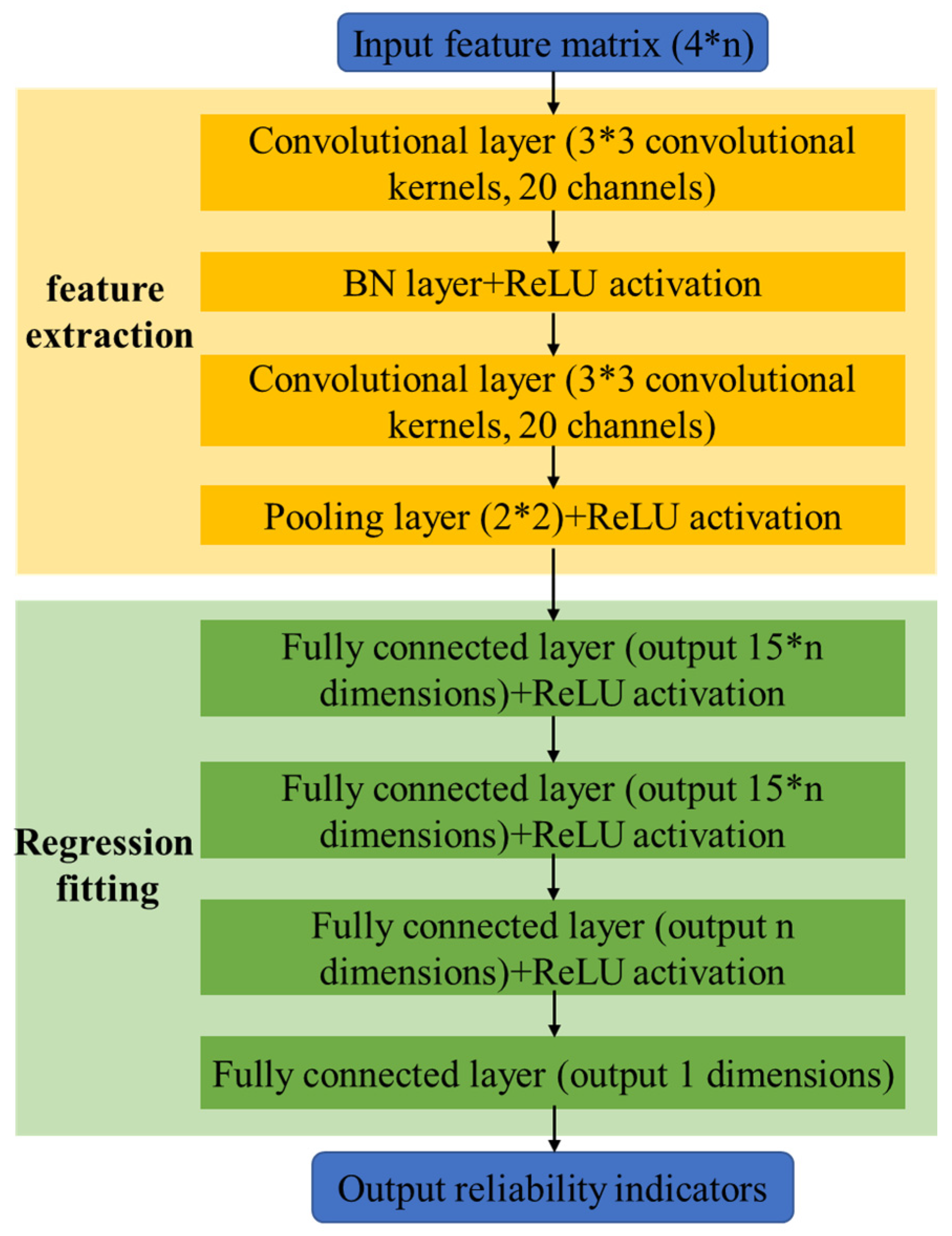
To obtain the mapping relationship between reliability indicators and system operating status (input feature matrix
X), a CNN-based regressor model is designed, as shown in
Figure 2. Among them, the kernel size of both convolutional layers is 3*3, and the number of channels is set to 20 and 40, respectively. At the same time, to accelerate neural network training, a BN layer was introduced to perform batch normalization on the features extracted by convolution. The output dimensions of the fully connected layer are 15n, 15n, n, and 1, respectively. The final output dimension is 1, and the output quantity is the system reliability index. The loss function of the regression model is as follows:
Here, Nr is the number of samples used for reliability evaluation regression training, is the actual reliability evaluation index value, is the reliability index value fitted by the CNN regression network, α is the weight coefficient, and wr is the weight matrix of the regression network. In practical applications, for specific power systems, a certain number of system operating state samples can be generated by solving the reliability analysis models (10)–(12), and the training of the regression network can be completed using known system operating states and reliability indicators as raw data. It should be noted that the BP algorithm has strong optimization capabilities. Through the backpropagation algorithm, the model can automatically adjust network parameters to reduce the value of the loss function, thereby improving the prediction accuracy of the model. In addition, the BP layer can also achieve complex nonlinear mapping relationships, enabling the model to handle various complex tasks. Therefore, when constructing deep learning models, CNN and BP layers are usually used in combination to improve the performance of the model.
3.3. Improved CNN Classification Regression Model
The uncertainty characteristics of power systems containing renewable energy are significant, and the fluctuation range of system operation status is large. The CNN regression model directly trained according to
Section 3.2 is difficult for achieving high-fitting accuracy on all the samples to be evaluated. Therefore, a CNN-based classification model is further introduced, which first classified the operating status samples based on whether they could be reliably powered, and then estimated the reliability indicators of the samples that could not be reliably powered, thus forming a CNN classification regression model. This processing is not only beneficial for improving the accuracy of CNN regression model training and reliability evaluation, but also avoids the evaluation and calculation of a large number of samples without load shedding, which helps to improve efficiency. At the same time, in practical applications, a more detailed classification of the system’s operating status can also be made based on the binary classification in this article, further improving regression accuracy.
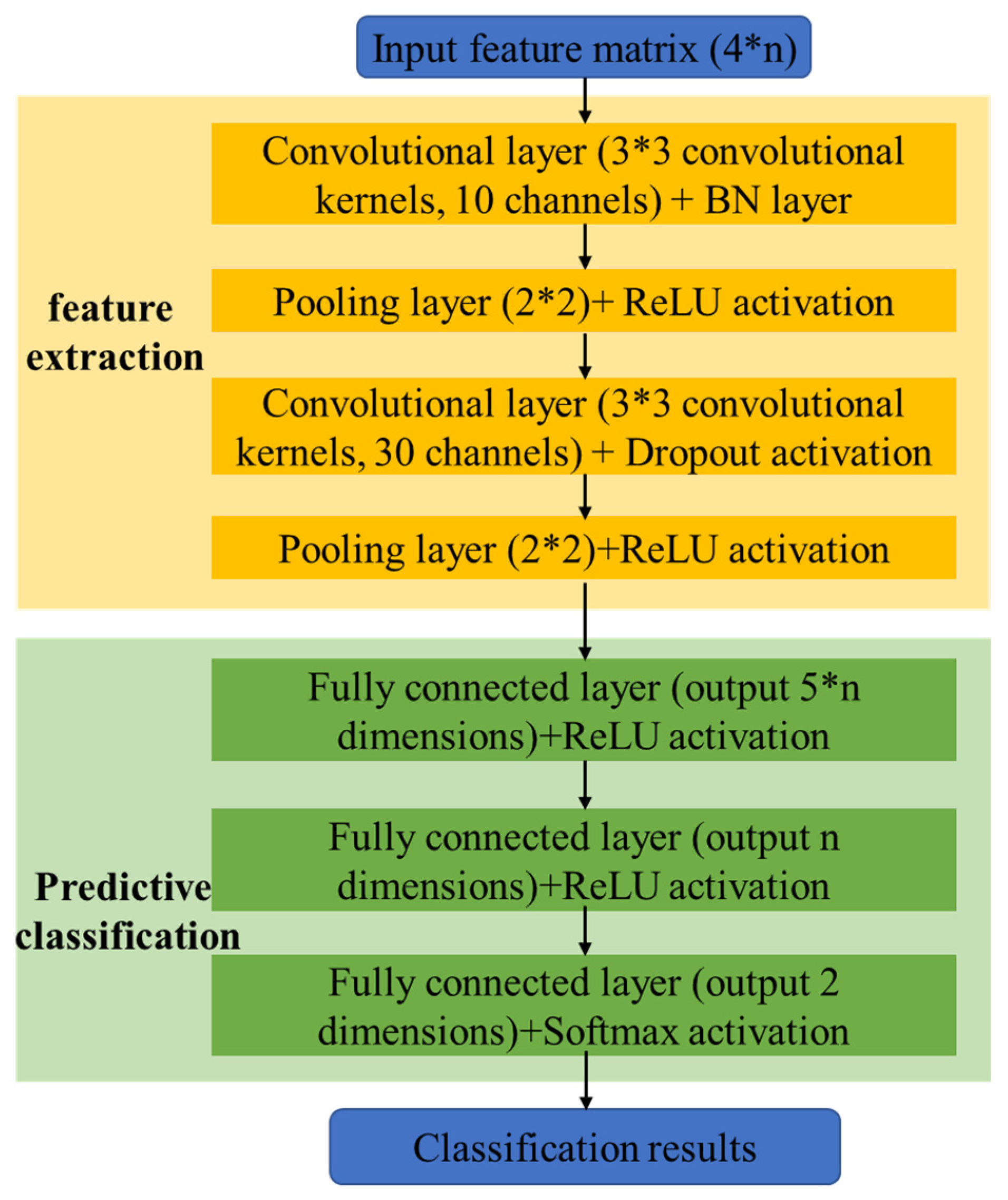
The input of the classification model is consistent with the regression model, that is, the input feature matrix
X established by Equation (20); but its output is the confidence level of whether the system can reliably supply power. To this end, a Softmax activation function is added before the final output of the classification network. Considering that sample classification is considered simpler than reliability index regression, in terms of network structure design, the classification model introduces an additional pooling layer and reduces a fully connected layer compared to the regression model. The overall structure is shown in
Figure 3. The loss function for classification is shown in Equation (22):
Here, Ncl is the number of samples used for classification training; y*cl,o is the 0–1 label; y cl o is the output of the classification model; β is the weight coefficient, and wcl is the weight matrix of the classification model neural network.
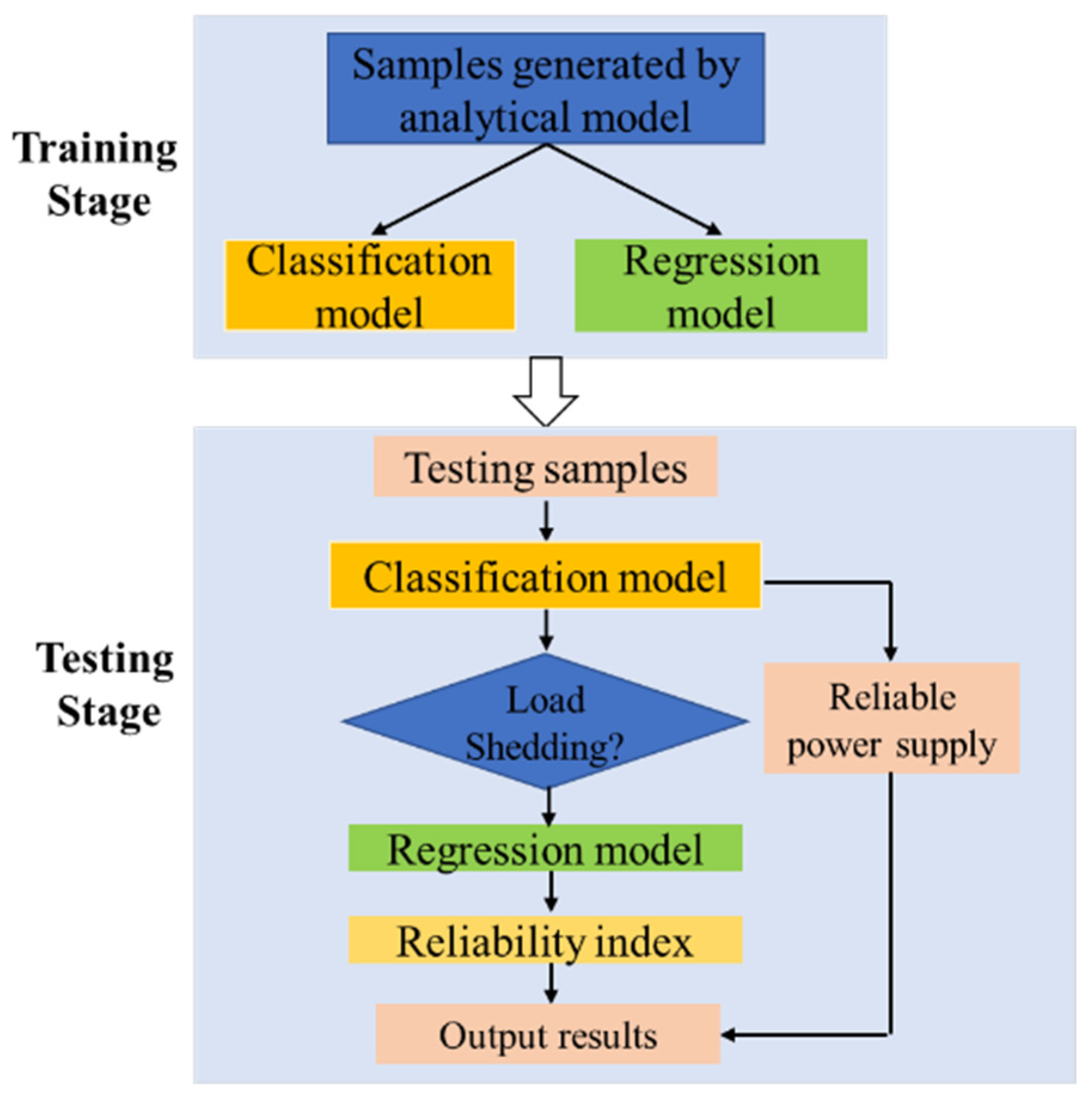
Finally, the combination of the classification model and regression model forms a CNN classification–regression model. The detailed calculation flowchart is shown in
Figure 4. During training, the classification model and regression model are two independent neural networks that can be trained separately. The classification model training set is filtered to obtain the regression model training set. After filtering, only a small portion of the samples with reliable power supply in this training set are used to improve the training efficiency and performance of the regression model. During testing, the two can be connected in series, and the system status can be classified first, followed by regression prediction of the load shedding of samples that cannot be reliably powered.
4. Case Study
4.1. Introduction of the Test System
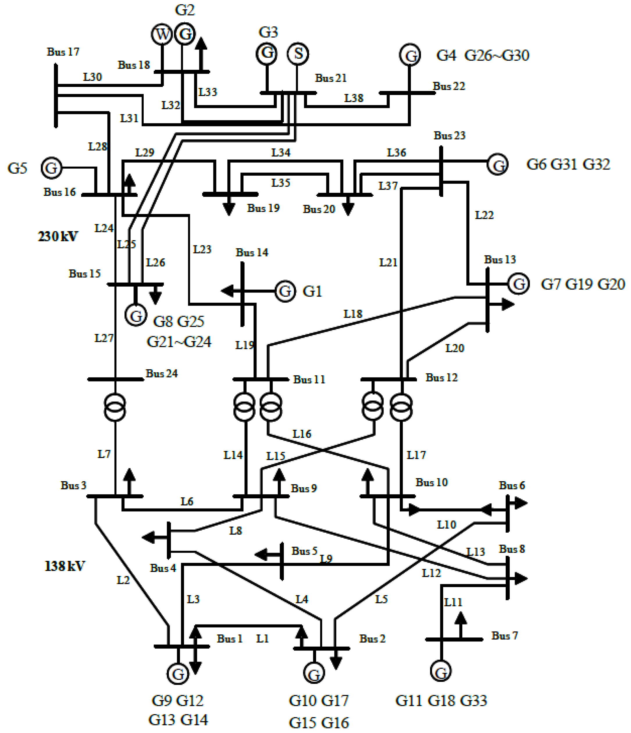
This article takes the RTS-79 testing system as an example. The RTS-79 testing system is widely used in power system reliability assessments due to its advantages of standardization, scale, data accessibility, and representativeness. The IEEE-RTS testing system wiring diagram is shown in
Figure 5, which includes 32 generators, 33 transmission lines, and 5 transformers. The total installed capacity of the system is 3405 MW, with a peak load of 2850 MW. The annual load curve and reliability parameters of each component are detailed in the literature [
13]. At the same time, in order to facilitate the verification of the effectiveness of the method proposed in this article in high-proportion renewable energy scenarios, 70 MW wind farms are added at nodes 15, 16, 18, 19, and 21, and 50 MW photovoltaic power plants are added at nodes 13, 17, 20, 22, and 23. The output curves of wind and photovoltaic power stations are based on statistical data from a certain province in northwest China and converted according to the installed capacity [
17]. Reliability assessments and CNN-related programs were written using software MATLAB 2016b. All calculations were conducted on a desktop computer with an Intel (R) Core (TM) i5-7500 CPU at 3.40GHz and 8 GB of memory.
4.2. Effectiveness Validation of Power System Reliability Assessment of Analytical Models
We constructed multiple reliability index analysis models through different component combinations, and calculated the corresponding reliability of these cases. The calculation results were compared with traditional reliability models to demonstrate the effectiveness and feasibility of the proposed model. The set cases are as shown in
Table 1.
When calculating the model coefficients, the availability of G13, G16, and G18 is set to 0.93, the availability of L13, L18, and L21 is set to 0.9994, and the variance coefficient of convergence accuracy is set to 0.010 After the above reliability evaluation analytical models are established, the reliability indicators of IEEE-RTS can be obtained by directly substituting the availability of the interested components into the corresponding models. By comparing the evaluation results with traditional Monte Carlo simulation methods, the accuracy of the proposed analytical model can be verified. For a more intuitive evaluation of accuracy, the relative error can be calculated using Equation (23):
The detailed calculation results are shown in
Table 2.
For the reliability evaluation of power systems based on Monte Carlo simulation, various computational efficiency improvement techniques have been proposed in existing research, including variance reduction techniques, system state analysis acceleration techniques, etc. However, these methods only limited the time required for a single reliability assessment, and repeated evaluations are still very time-consuming. An effective solution to these shortcomings is to establish an analytical calculation model for the variation in system/node reliability indicators with component reliability parameters. This paper uses the total probability formula and conditional probability to separate the reliability parameters to be solved from the reliability index calculation formulas, and establishes an explicit analytical model of system/node reliability index that includes component reliability parameters. In other words, analytical expressions can be seen as fitting the complex nonlinear relationship between reliability indicators and component parameters. In order to reduce computational complexity and improve computational efficiency, analytical models usually simplify the actual power system to a certain extent. These simplifications may lead to differences between the model and the actual system, thereby introducing errors. Regardless of whether the components of interest are generator sets, transmission lines, or both, the proposed analytical model obtains high accuracy reliability indicators, which can control the error within 1.5%.
On the other hand, by analyzing the model, the computational time of repetitive sequential Monte Carlo methods is also avoided. This section compares the time of two methods in scenarios where reliability parameters vary multiple times. For convenience, this section is not intended to solve a specific optimization problem. Instead, it is assumed that during the optimization process, 40 reliability evaluations need to be conducted for different availability rates of components in cases 1–6. By multiplying the original availability rates of G13 and G16 by 40 pre-set multipliers, a corresponding 40 sets of different availability rates are obtained. For the proposed model, several Monte Carlo simulations are required to determine the coefficients of the model. After determining the model coefficients, the corresponding reliability indicators can be obtained by directly substituting the repair time of each group of components in cases 1–6 into the analytical model.
Table 3 presents the proposed model and Monte Carlo method calculation time for 40 different repair times for components.
According to
Table 3, in order to obtain all the reliability evaluation results, the calculation time for Monte Carlo simulation is about 30 days, while the proposed model only takes about 3 days. This is because for each set of component repair times, the former requires running a sequential Monte Carlo simulation once. However, the proposed analytical model only requires 5 temporal Monte Carlo simulations to determine the coefficients of the model. After the coefficients are determined, the reliability evaluation based on the analytical model takes very little time, and the total evaluation process time does not exceed 1 s. The results in
Table 3 indicate that once the analytical model is established, the reliability indicators for the given reliability parameters can be directly obtained without the need for time-consuming Monte Carlo simulations.
4.3. Feasibility Verification of CNN Classification Regression Model
To demonstrate the effectiveness of the CNN classification regression method, the following six methods were compared on the test set formed in
Section 4.2.
M1: Solve the traditional MCS model as a reference value.
M2: Train a CNN regression model using the two-dimensional matrix vector mentioned in this article as input.
M3: Train a CNN classification regression model using the two-dimensional matrix vector proposed in this article as input.
M4: The two-dimensional matrix vector proposed in this article is transformed into one-dimensional as the input for DNN, and the DNN classification regression model is trained.
M5: Use 0–1 variables to represent the status of generators and transmission lines, and use them as inputs to the DNN along with node load and renewable energy output to train the DNN classification regression model.
Among them, the learning rate of the classification model is taken as 0.0005, β is taken as 0, and the batch size is taken as 50. The SGD gradient descent algorithm is used to iterate 500 epochs. The learning rate of the regression model is taken as 0.005, a is taken as 0.2, and batch size is taken as 50. The Adam optimization algorithm is used, and the convergence criterion is that the loss function is less than 0.8 or reaches 2500 epochs. The structure of a DNN is the same as the fully connected layer in a CNN, and the activation function, optimizer, and learning rate are also consistent with the CNN model.
The accuracy index
Pacc and F1 score (F1) are used to evaluate the performance of the classification model, and the calculation method is shown in Equations (24) and (25):
Among them,
TP is the correctly judged unreliable power supply sample,
TN is the correctly judged reliable power supply sample,
FP is the misjudged unreliable power supply sample, and
FN is the misjudged reliable power supply sample. The performance of the regression model is evaluated using the average absolute percentage error E
MAPE and the weighted average absolute percentage error E
WMAPE, as shown in Equations (26) and (27):
Here, Nt is the number of test samples. It should be noted that only the LOLP indicator is calculated here. The LOLF and EENS indicators can also be obtained based on this model.
Due to the significant uncertain characteristics of the system and the large range of operating state fluctuations, introducing necessary classification mechanisms before regression analysis can achieve more accurate regression results than just using a regressor, as shown in the comparison of M1 and M2 results in the
Table 4. Comparing M2, M3, and M4, it can be found that among several common deep learning methods, CNN has the best-fitting effect, with a classification accuracy of 99.64% and a loss of load estimation deviation of only 1.42%. By comparing M3 and M5, it can be found that the input feature vectors designed in this paper contain specific system parameter information (such as generator capacity, etc.), which is more effective than simply using 0–1 variables to represent component state information, achieving higher accuracy and precision.
At the same time, the time required for M1–M5 to evaluate the test set samples was compared. M1 took 1042.21 s to calculate the optimal load shedding model, while M2 took 13.36 s, which is only 1/78 of M0. At the same time, the time consumption of M3, M4, and M5 is 19.09 s, 16.78 s, and 14.87 s, respectively, and there is no significant difference in time consumption compared to M2. Considering the accuracy requirements, overall, the method M2 proposed in this article can maintain high solving accuracy while having good acceleration effects.
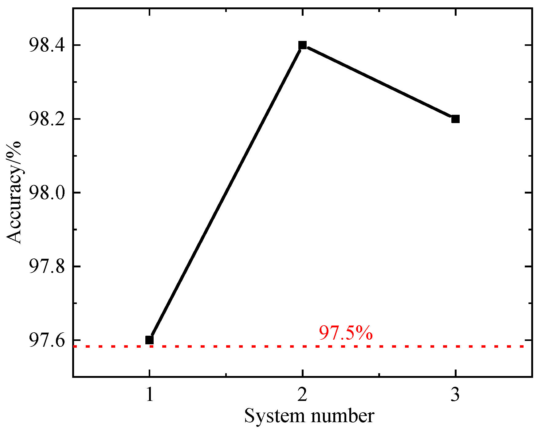
Furthermore, three different scale testing systems, including the Reliability Test System (IEEE RTS), Western Systems Coordinating Council (WSCC) Test System, and an actual provincial power grid in southwestern China, are used to verify the feasibility of the proposed model. The above three testing systems are named system 1, 2, and 3, respectively. Firstly, the actual reliability parameters are obtained using Monte Carlo simulation, and then the reliability parameters under the same operating conditions are obtained using the data-driven strategy proposed in this paper. The accuracy is calculated by comparing the results obtained by different methods. The detailed calculation results are shown in
Figure 6. It can be observed from
Figure 6 that the method proposed in this paper can still achieve high computational accuracy, with a calculation accuracy of over 97.5%, while significantly improving computational efficiency, meeting the needs of practical engineering applications.
5. Conclusions
In the process of solving the inverse problem of reliability evaluation, sometimes it is necessary to use Monte Carlo simulation to perform multiple reliability evaluations on different values of the reliability parameters to be solved, which is extremely time-consuming. In response to the above issues, this chapter proposes an analytical model for reliability indicators related to component reliability parameters based on time-series MCS. Then, an input feature vector reflecting the operating status of the system was constructed, and a reliability index regression model based on a CNN was constructed. Secondly, in response to the diverse operating scenarios of the system, it is extended to a CNN classification–regression model to improve training efficiency and accuracy. The calculation results indicate the following.
- (1)
The proposed reliability index analysis model can intuitively display the functional relationship between reliability indicators and the reliability parameters to be solved. The proposed analytical model can accurately and efficiently calculate the system reliability indicators that vary with the reliability parameters of the components, with an error of no more than 2% compared to the Monte Carlo simulation.
- (2)
The proposed CNN classification–regression model can significantly improve computational efficiency while ensuring computational accuracy, with a computation time for only 1.3% of the traditional Monte Carlo simulation method.
Most existing reliability assessment methods for power systems focus on reliability assessment at a single time scale, such as long-term or short-term reliability, etc. However, in practical operation, the power system may face reliability issues at multiple time scales simultaneously. Therefore, studying how to comprehensively consider the reliability of multiple time scales and establish a multi-time scale reliability evaluation method for power systems is a challenging and practical research direction. On the other hand, the current power system is gradually transitioning towards the integrated energy system, and the complexity of the system is further increasing. How to establish a reliability evaluation model suitable for integrated energy systems is also a focus of future research.


