Enhancing Control Room Operator Decision Making

Abstract

In the dynamic and complex environment of industrial control rooms, operators are often inundated with numerous tasks and alerts, leading to a state known as task overload. This condition can result in decision fatigue and increased reliance on cognitive biases, which may compromise the decision-making process. To mitigate these risks, the implementation of decision support systems (DSSs) is essential. These systems are designed to aid operators in making swift, well-informed decisions, especially when their judgment may be faltering. Our research presents an artificial intelligence (AI)-based framework utilizing dynamic influence diagrams and reinforcement learning to develop a powerful decision support system. The foundation of this AI framework is the creation of a robust, interpretable, and effective DSS that aids control room operators during critical process disturbances. By incorporating expert knowledge, the dynamic influence diagram provides a comprehensive model that captures the uncertainties inherent in complex industrial processes. It excels in anomaly detection and recommending optimal actions. Furthermore, this model is improved through a strategic collaboration with reinforcement learning, which refines the recommendations to be more context-specific and accurate. The primary goal of this AI framework is to equip operators with a live, reliable DSS that significantly enhances their response during process upsets. This paper describes the development of the AI framework and its implementation in a simulated control room environment. Our results show that the DSS can improve operator performance and reduce cognitive workload. However, it also uncovers a trade-off with situation awareness, which may decrease as operators become overly dependent on the system’s guidance. Our study highlights the necessity of balancing the advantages of decision support with the need to maintain operator engagement and understanding during process operations.

1. Introduction

In recent years, the industrial landscape has undergone a significant transformation with the advent of Industry 4.0, also known as the fourth industrial revolution [1]. First introduced at Hannover Messe 2011 in Germany, Industry 4.0 marks a new era in intelligent manufacturing, characterized by the integration of advanced technologies and data-driven decision making. This paradigm shift aims to enhance productivity, effectiveness, and competitiveness across many industries, from automotive manufacturing and aerospace to ch and revised all. and renewable energy sectors [2]. Central to this transformation is the adoption of decision support systems (DSSs), which are pivotal in facilitating informed and optimized decision-making processes. The contemporary industrial environment, characterized by its complexity and dynamism, necessitates intelligent DSSs capable of managing vast amounts of information, modeling intricate systems, and supporting operators effectively [3]. Al-Dabbagh et al. (2018) [4] emphasize the significant role of Decision Support Tools in enhancing the control and operation of industrial facilities.

A critical aspect of a DSS is its dual nature, encompassing both technical and human factors. The primary consideration in DSS usage is the human element. These systems are designed to assist, not replace, human decision makers [5]. Developing a model that can process large volumes of data and efficiently convey information to operators is a complex task. The effectiveness of a DSS in enhancing operator performance is not guaranteed and requires careful construction [6]. Constructs such as situation awareness (SA), mental workload, and trust are crucial in understanding and predicting human-system performance in complex environments [7]. The process of trust calibration plays a critical role in the usage of DSS and human operator [8]. The technical challenge in building a DSS is equally significant. Generally, there is a reluctance to adopt systems that are not directly interpretable, tractable, and trustworthy, particularly in safety-critical contexts [9]. Thus, there is a pressing need for models that are not only effective in handling large data volumes but also interpretable and safe. Trustworthy and effective models are essential.

In the context of contemporary chemical processes, there is a strong reliance on automation via distributed control systems [10]. Routine adjustments to expected process variations are overseen by process logic controllers (PLCs), which remotely control equipment components like valves and motor drives. At the core of industrial operations, operators interact with a graphical user interface (GUI) that aggregates and displays signals from instruments attached to machinery. Occasionally, system parameters might deviate beyond the set thresholds in the PLCs, triggering alarm notifications on the GUI. These alarms demand the operators’ attention. Using the GUI’s data, operators are responsible for diagnosing the irregularity and deciding on the necessary actions to restore balance in the process. This diagnostic and corrective process demands intricate cognitive processing, urging operators to synthesize multiple data points, account for external factors like weather conditions, and predict the potential outcomes of each possible action [11]. Such situations can quickly become overwhelming for operators, making decisions susceptible to cognitive biases rather than comprehensive assessments. In these critical moments, the importance of decision support tools becomes evident. In developing a decision support system (DSS) for a chemical plant, our approach aligns with the principles outlined by Lee and Seong (2012), who emphasized the importance of identifying abnormal operating procedures in safety-critical environments, such as nuclear power plants, to enhance operational safety and efficiency [12].

Creating an effective decision support system (DSS) for control room operators involves balancing high performance with clear interpretability while also considering the unique needs and behaviors of human operators. The system must efficiently process large data volumes, provide understandable insights, and integrate seamlessly with existing workflows. It is crucial that the DSS enhances decision making without overwhelming the operators, ensuring it becomes a trusted and valuable tool in high-stakes environments.

1.1. Literature Review

The fusion of intelligent systems within manufacturing and the wider realm of operations management has traditionally been seen as a beneficial confluence of operational research (OR) and AI. This collaborative potential is emphasized in studies by [13,14]. Additionally, ref. [15] emphasized the escalating inclination towards the adoption of AI methodologies in this domain.

Hsieh et al. (2012) [16] address a critical aspect of nuclear power plant (NPP) safety. They focus on the development of a decision support system intended to aid operators in quickly and accurately identifying abnormal operating procedures (AOPs) in NPPs. The study stands out for its emphasis on reducing the complexity of decision-making processes, particularly in the high-stress environment of NPP control rooms. A significant contribution of the paper is the integration of a comprehensive abnormal symptom database into the decision support system, which allows operators to filter out irrelevant information and prioritize critical alarms. This approach is designed to improve the accuracy and speed of identifying appropriate AOPs, thereby enhancing the overall safety and effectiveness of NPP operations. Importantly, the authors conducted an experiment involving graduate students simulating NPP operators to validate the system’s effectiveness. The results indicated a reduction in decision-making time and errors as well as a decrease in the mental workload of operators using the system, but the study did not assess SA. This evidence emphasizes the potential of the decision support system as a valuable tool in NPPs.

Kang and Lee (2022) [17] outline the limitations of existing emergency operating procedures (EOPs), which often fail to adapt to the dynamic nature of emergency situations, increasing the cognitive workload on operators and the potential for human error. The emergency guidance intelligent system (EGIS) they developed aims to overcome these limitations by providing agile, dynamic, and intuitive operations. It assists operators by automating the monitoring of plant status, identifying current and latent risks, and presenting this information in a clear and actionable manner. A key feature of the EGIS is its ability to reduce the workload on operators by prioritizing tasks and presenting only the most relevant information, thus potentially reducing the time required for initial emergency response. However, SA was also not assessed. The system was rigorously tested in various simulated emergency scenarios, demonstrating its effectiveness in improving response times and reducing operator workload compared to traditional procedures.

One important limitation of these two studies is that their methods are based on a rule-based system, which makes them difficult to apply if the situation is uncertain. One very effective and interpretable model to use for decisions under uncertainty are Bayesian networks [18,19]. Bayesian networks have been used in fault detection, diagnosis, prognostics, and also root cause analysis [20], but there are not many reported applications of Bayesian networks in the industry, or they are only mentioned as knowledge-based systems, as mentioned in [21]. On the other hand, Bayesian networks are a very promising tool for building a powerful and trustworthy DSS. Some industrial applications were tested.

In the study by Weidl et al. (2005) [22], a versatile methodology for root cause analysis and decision support in industrial process operation is introduced. The authors effectively demonstrate how object-oriented Bayesian networks (OOBNs) [23], ref. [24], can be utilized to model complex dependencies and uncertainties inherent in industrial systems, thereby providing a robust framework for decision support. The study meticulously illustrates the potential of OOBNs in capturing the intricate interdependencies within industrial processes, emphasizing their utility in predictive maintenance and operational effectiveness. A key contribution of the paper is the demonstration of OOBNs as a flexible and dynamic tool, adaptable to the diverse and evolving nature of industrial operations. The authors present a compelling case for the use of OOBNs in decision making, highlighting their superiority over traditional methods in handling uncertainty and complexity. This is particularly pertinent in the context of industrial asset management, where the ability to predict and manage potential failures and optimize operational performance is crucial. The paper also thoughtfully discusses the challenges and limitations associated with implementing OOBNs in industrial settings, such as the need for high-quality data, the complexity of model construction and interpretation, and the integration with existing industrial systems.

Horvitz and Barry (2013) [25] extensively utilize Bayesian networks and influence diagrams to innovate in the realm of time-critical decision-making processes. Their study emphasizes the effectiveness of these tools in evaluating the trade-offs between the promptness of actions and their potential outcomes, especially in dynamic settings where decisions are both urgent and consequential. They propose a decision-theoretic approach to the design of interfaces capable of integrating and displaying complex probabilistic dependencies in real time. This methodology is crucial in areas where making timely decisions is essential, leading the way for the development of systems that can more efficiently assist human operators by providing information tailored for swift and well-informed decision making.

However, a notable limitation of both studies is the lack of participant-based testing to empirically evaluate the actual impact on human performance, workload, and situational awareness.

In [26], Abbas et al. address a critical challenge in the realm of safety-critical systems: the difficulty in identifying the physical model of complex systems and the limitations of deep reinforcement learning (DRL) in these contexts. The paper proposes an innovative approach that combines the advantages of probabilistic modeling with reinforcement learning, thus providing a novel solution to enhance decision making in safety-critical systems. The core of their proposed methodology, the behavioral cloning-based specialized reinforcement learning agent (BC-SRLA), seeks to integrate these approaches into a hierarchical framework. This architecture not only leverages the strengths of probabilistic modeling and reinforcement learning but also incorporates elements of interpretability and minimal interaction with the environment. This approach is particularly aimed at addressing the challenges associated with using RL in safety-critical industries. This shows the potential of the use of a probabilistic model with RL [27,28,29].

1.2. Contribution

This research represents a notable advancement in the field of decision support systems (DSSs) and is specifically designed for control room operations in safety-critical sectors. We devised a DSS that is not only effective but also interpretable, ingeniously fusing the strengths of Bayesian networks and reinforcement learning. This innovative approach leverages the predictive capabilities of Bayesian networks to precisely model intricate systems and their inherent uncertainties. Simultaneously, reinforcement learning enhances the system’s adaptability and accuracy, facilitating more precise decision making. The methodology described in this study serves as an extensive framework for building an AI system that effectively captures the physical behavior of processes and their uncertainties. This is vital for the development of a robust and dependable DSS. Additionally, the integration with reinforcement learning is elaborately explained, contributing to the formation of a potent and precise DSS. The combination of Bayesian networks and reinforcement learning not only improves the system’s predictive accuracy but also ensures its practicality and applicability in real-world, safety-critical contexts.

The other key contribution of our work is the empirical validation of the developed framework through a structured experimental study involving participants from diverse backgrounds. This hands-on testing approach provides a comprehensive assessment of the system’s impact on various critical aspects of control room operations, including operator performance, workload, situation awareness, and physiological responses. By engaging participants in simulated scenarios that mimic real-world challenges, we have been able to gather valuable data and insights into the practical application and effectiveness of the decision support system. Furthermore, the physiological measurements collected during the experiment provide an objective assessment of the system’s impact on the operators. This aspect of our study is particularly noteworthy as it offers a quantifiable measure of the physiological responses to using the decision support system.

1.3. Structure

This paper is a combined and extended version of papers published in conferences about this experiment; see [30] for the construction of the dynamic influence diagram and ref. [31] for the AI framework. In this paper, we commence by delineating the methodology employed, encompassing both the experimental design and the mathematical approaches utilized. Subsequently, we explain the construction of a decision support system grounded in dynamic influence diagrams and reinforcement learning and provide a detailed description of the comprehensive AI framework we developed. Following this, we present the application and evaluation of this framework through experimental testing. We discuss the results and their implications. This paper concludes with a summary of our findings and reflections on their significance and on future work.

2. Materials and Methods

2.1. Experimental Setup

The basis of our experiment is a simulator designed for formaldehyde production [32]. This simulator is customized to replicate the environment of a control room. A key enhancement to this setup is the “support panel”, which transforms the simulator into a comprehensive control room simulation. This panel includes various features: a graphical display for production monitoring, an alarm list, a procedure list, and an automated suggestion feature. In terms of process, the plant simulates a production rate of 10,000 kg/h of 30% formaldehyde solution, produced by the partial oxidation of methanol with air. The simulator consists of six sections: tank, methanol, compressor, heat recovery, reactor, and absorber. It also includes 80 alarms of different priority levels, along with nuisance alarms (irrelevant alarms). The main screen of the simulator is shown in Figure 1, and the detailed tank mimic is displayed in Figure 2. The support panel is shown in Figure 3. To evaluate the effectiveness of the developed decision support, three scenarios are defined:

• Pressure indicator control failure: In this scenario, the automatic pressure management system in the tank stops working. As a result, the operator must manually adjust the nitrogen inflow to maintain the correct pressure. Here, the cessation of nitrogen flow leads to a pressure drop as the pump continues to supply nitrogen to the plant.
• Nitrogen valve primary source failure: This scenario is a variation of the first one in which the tank’s primary nitrogen source fails. The operator is required to switch to a backup system. As the backup system initiates slowly, the operator needs to control the pump power to reduce the rate of pressure decline in the tank.
• Temperature indicator control failure in the heat recovery section: Initially, the operator tries to solve the problem by manually adjusting the cooling water flow set point in the absorber. When this fails, the operator consults the supervisor for advice. The supervisor indicates that the issue cannot be resolved from the control room and requires a field operator’s intervention. While the field operator attends to the problem on-site, the control room operator must manage the reactor’s temperature. The main challenge in this scenario is preventing the reactor from overheating, necessitating close monitoring and adjustment of the reactor’s cooling water temperature.

2.2. Digitized Screen-Based Procedures

Procedures are crucial for control room operators to ensure process safety. However, shortcomings exist in both the design and operator usage of these procedures, leading to major accidents in safety-critical sectors such as the nuclear and oil and gas industries. Notable examples include the Piper Alpha Platform explosion and the Longford Gas Plant 1 explosion and fire [33]. Issues with procedures, such as being outdated, overly voluminous, or poorly represented, have necessitated different designs and updates, including the adoption of computerized procedures or flowchart representations.

This study introduces a screen-based digitized procedure, designed by [34], for comparison with an AI-based procedure support. The digitized procedure employs a hierarchical, rule-based task representation format, detailing each step to resolve plant alarms. The procedure for each alarm is organized for easy navigation on a support display, as illustrated in the top-right corner of Figure 3.

2.3. Dynamic Influence Diagrams

This section aims to clarify the fundamental principles behind dynamic influence diagrams (DIDs). Our discussion begins with an examination of Bayesian networks (BNs), laying the groundwork for understanding DIDs. We then delve into influence diagrams, a specialized form of BNs, to grasp their structure and operational mechanisms. Ultimately, we introduce the element of dynamism to these diagrams, culminating in a thorough understanding of dynamic influence diagrams and their role in intricate decision-making scenarios.

2.3.1. Bayesian Network

A Bayesian network serving as a domain model is fundamentally a graphical structure composed of nodes and connecting arcs. The nodes represent domain concepts or variables, while the arcs symbolize the interactions among these nodes. These interactions are quantitatively described using conditional probabilities, capturing the dependencies between different domain elements [35]. This model is employed for decision making, prediction, and inference, modeling the probabilistic connections among various variables [36]. In the graph, each node symbolizes a variable, and the edges reflect the conditional dependencies. The strengths of these dependencies are quantified using conditional probabilities.

The following definition is provided by Jensen and Nielsen [18]:

Definition 1

(Discrete Bayesian network). A discrete Bayesian network $\mathcal{N}=(X,G,P)$ is composed of the following:

• A DAG $\mathcal{G}=(V,E)$, where $V=v_1,...,v_n$ represents the nodes and E denotes the directed links.
• A set of discrete random variables, $\mathcal{X}$, each of which is represented by a node in $\mathcal{G}$.
• A set of conditional probability distributions, $\mathcal{P}$, with each distribution $P\left(X_v\right|X_{pa\left(v\right)})$ corresponding to a random variable $X_v\in \mathcal{X}$.

A Bayesian network encodes a joint probability distribution over a set of random variables, $\mathcal{X}$, of a problem domain. The conditional probability distributions, $\mathcal{P}$, define a multiplicative factorization of the joint probability distribution over $\mathcal{X}$:

$$P\left(\mathcal{X}\right)=\prod _{(v\in V)}P\left(X_v\right|X_{pa\left(v\right)})$$

(1)

2.3.2. Influence Diagrams

An influence diagram is a probabilistic graphical model that represents relations between chance variables and decision nodes in a decision-making process [37]. It is a Bayesian network augmented with decision nodes and utility functions, aiding in decision making under uncertain conditions. Decision nodes symbolize the choices or actions available to a decision maker; chance variables denote uncertain events or states; and utility functions reflect the values or preferences from the decision maker’s point of view linked to various outcomes. Influence diagrams offer a systematic approach for modeling and analyzing complex decision scenarios, enabling decision makers to compute the expected utility of different options and make well-informed choices. A limited-memory influence diagram, as described in [38], modifies the conventional influence diagram model by relaxing the assumptions of perfect recall of past events and the strict sequence of decisions. The discrete limited-memory influence diagram is defined as follows:

Definition 2

(Discrete limited-memory influence diagram [39]). A discrete limited-memory influence diagram, denoted as $N=(X,G,P,U)$, is composed of the following:

• A directed acyclic graph (DAG) $G=(V,E)$, with nodes V and directed edges E. This graph represents dependence relations and information precedence among variables.
• A set of discrete random variables $X_C$ and discrete decision variables $X_D$, where $X=X_D\cup X_C$. These variables are represented by the nodes of G.
• A set of conditional probability distributions P containing one distribution $P\left(X_v\right|X_{pa\left(v\right)})$ for each discrete random variable $X_v$ given its parents $X_{pa\left(v\right)}$.
• A set of utility functions U containing one utility function $u\left(X_{pa\left(v\right)}\right)$ for each node v in the subset $V_U\subseteq V$ of utility nodes.

To determine the option of a decision variable with the highest expected utility, we calculate the expected utility for each decision alternative. Given a decision variable A with options $a_1,\cdots ,a_m$, a hypothesis H with states $h_1,\cdots ,h_n$, and a set of observations $ϵ$ as evidence, then we can compute the utility of each outcome of the hypothesis and the expected utility of each action, The utility of an outcome $(a_i,h_j)$ is given by $U(a_i,h_j)$, where $U(·)$ represents the utility function. The expected utility of taking action $a_i$ is calculated by

$$\mathbb{EU}\left(a_i\right)=\sum _{j=1}^{n}U(a_i,h_j)P\left(h_j\right|ϵ)$$

(2)

In this equation, $P(·)$ indicates our belief in hypothesis H given the evidence $ϵ$. The utility function $U(·)$ quantifies the decision maker’s preferences on a numerical scale.

To select the optimal decision, we apply the principle of maximum expected utility, which involves choosing an option $a^{\ast }$ such that

$$a^{\ast }={\mathrm{argmax}}_{a_i\in A}\mathbb{EU}\left(a_i\right)$$

(3)

2.3.3. Dynamic Influence Diagram

Dynamic influence diagrams incorporate discrete time into the model. This time-sliced approach is based on a static network, where each time slice maintains a static structure [40]. The evolution of the system over time is defined by the connections between variables of different time slices. Temporal links within a time slice consist of connections from variables of the preceding time slice to those of the current one. The interface of a time slice is the set of variables that have parents in the preceding slice. In essence, a dynamic model can be visualized as a series of static models ordered sequentially, each representing the system’s state at a specific time step. The links between time steps define the impact of the system’s past state on its present state, as shown in Figure 4 [39]. For our experiment, we utilized a finite horizon dynamic influence diagram.

In Figure 5, the structure of a basic dynamic influence diagram (DID), managed using HUGIN software [41], is illustrated. This diagram includes several nodes:

• Decision node (depicted in pink): Represents the range of decision options available to an operator at a given point in time where a decision must be made. Each state of this node directly influences the distribution of physical values within the system, demonstrating the impact of an operator’s decisions on the process.
• Physical value node: Models the physical parameters of the system using states represented as intervals. This discretization is crucial for simplifying the model while retaining essential details. States indicating hazardous conditions in this node increase the likelihood of adverse outcomes.
• Consequence node: Encompasses potential outcomes or consequences (e.g., tank explosion or tank implosion) resulting from the system’s current state. Each state in this node is linked to a specific cost, reflecting the severity or impact of that outcome.
• Utility node (colored in green): Integrates the cost (or reward) of each potential consequence. The utility value is calculated by considering the probability of each consequence and its associated cost, quantifying the overall risk or benefit of a particular system state.
• Physical value node with stripes: Represents the physical values from the previous time step. Its function is to model the impact of past states on the current situation. This node is linked to the current physical value node, illustrating how previous states influence present conditions. Additionally, it is connected to the decision node, which is crucial for modeling informed decision-making processes in future time steps. By incorporating the previous physical values into the decision-making process, the model can predict the most appropriate actions based on the previous state of the “Physical value” node. This approach enables the construction of a comprehensive scenario where optimal decisions are made at each step, considering both past and present conditions.

The primary goal of this DID is to forecast future physical values and use these predictions to guide the operator to make the best possible decision.

2.3.4. Conflict Analysis

An anomaly is detected when a variable deviates from its intended set point or the default value predetermined by the automatic control mode. For anomaly detection, we apply conflict analysis as outlined in [42] within the influence diagram framework. In this context, conflict arises when the evidence propagated through the model shows inconsistencies or contradictions. More precisely, a conflict is assumed when the product of the individual probabilities of each piece of evidence is higher than the joint probability of the evidence. Consider a set of evidence, $ϵ=({ϵ}_1,\cdots ,{ϵ}_n)$. The measure of conflict is defined as follows:

$$\mathrm{conf}\left(ϵ\right)=\mathrm{conf}\left([{ϵ}_1,\cdots ,{ϵ}_n]\right)=log\left(\prod _i^n\frac{P\left({ϵ}_i\right)}{P\left(ϵ\right)}\right)$$

(4)

A conflict is flagged when $\mathrm{conf}\left(ϵ\right)>0$. A conflict can often be resolved by a hypothesis, denoted by h, with a low probability of occurrence prior to observing $ϵ$ and a high probability after observing $ϵ$. If $\mathrm{conf}(ϵ\cup h)<0$, it implies that h resolves the conflict. In our model, h represents a fault within the system. Consequently, if a fault resolves the conflict, it is detected and identified as a resolution of the conflict.

2.4. Deep Reinforcement Learning (DRL)

In recent years, the integration of deep reinforcement learning (DRL) techniques has revolutionized decision support systems, particularly in the realm of process control [43]. Process control involves the management and optimization of complex systems, where traditional control methods may fall short in addressing the complexities and uncertainties inherent in real-world processes. By leveraging the power of DRL, which combines deep neural networks with reinforcement learning algorithms, we aim to enhance the adaptability, effectiveness, and robustness of decision making in dynamic and uncertain environments.

DRL is a paradigm at the intersection of artificial intelligence, machine learning, and control systems [44]. It represents a powerful approach for training agents to make sequential decisions in complex and dynamic environments. At its core, DRL integrates deep neural networks to approximate complex functions and reinforcement learning algorithms to enable agents to learn optimal policies through interaction with their environment. Mathematically, the fundamental formulation of reinforcement learning involves the concept of Markov decision processes (MDPs), where an agent interacts with an environment by taking actions based on its current state, receiving rewards, and updating its policy to maximize cumulative future rewards. The Q-value function, denoted as Q(s, a), represents the expected cumulative reward of taking action “a” in state “s” and following the optimal policy thereafter. The Bellman equation, a cornerstone in reinforcement learning, expresses the recursive relationship between Q-values:

$$Q(s,a)=\mathbb{E}[r+\gamma \underset{a^{\prime }}{max}Q(s^{\prime },a^{\prime })|s,a]$$

(5)

Twin Delayed Deep Deterministic Policy Gradient (TD3) Architecture

One notable advancement in DRL is the twin delayed DDPG (TD3) architecture [45], designed to address challenges such as overestimation bias and brittle training. TD3 was used in our framework as the base DRL architecture. TD3 incorporates twin Q-value estimators to mitigate overestimation errors and a delayed policy update mechanism for stabilizing the learning process. The TD3 algorithm introduces the following key equations:

Critic update:

$$\mathcal{L}\left({\theta }_Q\right)={\mathbb{E}}_{(s,a,r,s^{\prime })\sim \mathcal{D}}\left[\frac{1}{2}{(Q_{1-\mathrm{target}}(s,a)-y)}^2\right]$$

(6)

$$y=r+\gamma (1-d)\underset{i=1,2}{min}{Q}_i$$

(7)

Policy update:

$$\mathcal{L}\left({\theta }_{\pi }\right)=-{\mathbb{E}}_{s\sim \mathcal{D}}\left[Q_1(s,\pi \left(s\right))\right]$$

(8)

where:

• $L\left({\theta }_{\pi }\right)$: the loss function with respect to the parameters ${\theta }_{\pi }$.
• $Q(s,a)$: expected cumulative reward for action a in state s.
• ${\mathbb{E}}_{s\sim \mathcal{D}}$: the expected value over states sampled from the distribution $\mathcal{D}$.
• r: immediate reward obtained from taking action a in state s.
• $\gamma$: discount factor for future rewards.
• ${max}_{a^{\prime }}Q(s^{\prime },a^{\prime })$: maximum expected future reward in the next state $s^{\prime }$.
• $Q_{1-\mathrm{target}}(s,a)$: predicted Q-value by the target critic network.
• y: target value for the critic update.
• $s,a,r,s^{\prime }$: state, action, reward, and next state, sampled from replay buffer.
• ${\pi }_{\mathrm{target}}\left(s^{\prime }\right)$: action selected by the target policy in the next state.
• $Q_1(s,\pi \left(s\right))$: Q-value associated with the selected action and state.
• $\pi \left(s\right)$: action selected by the policy in the current state.
• d: binary variable indicating whether the next state is a termination state or not.

These equations encapsulate the optimization objectives for updating the critic and policy networks within the TD3 architecture, providing a solid foundation for understanding its theoretical underpinnings and subsequent practical implications in the context of process control decision support systems.

2.4.1. DRL for Process Control

Authors in [46] focused on the use of DRL in the process control environment. The following state, action, and reward are formulated in our case following the literature [43].

State

In the context of a partially observable Markov decision process, relying solely on the observed state may be inadequate due to the system’s inherent partial observability constraints. Consequently, the state perceived by the DRL system differs from the actual environment state. To overcome this challenge, the investigation employs a tuple comprising the history of expert actions concatenated with the history of process variables. This history can extend up to a length denoted as “l”, as illustrated in Equation (9). The selected historical information encompasses the current state at time “t” and only the preceding trajectory at time “t − 1”:

$$s_t:=〈\left(y_{t-l},a_{t-l-1}^E\right),\dots ,\left(y_t,a_{t-1}^E\right)〉$$

(9)

Action

The actor network in reinforcement learning is responsible for determining the policy, which is essentially the mapping from states to actions. In the context of the TD3 architecture, the actor network typically outputs a continuous action parameterized by a neural network. The actor’s output can be denoted as follows:

$${\pi }_{\theta }\left(s\right)=\mu \left(s\right)$$

(10)

Here, $\mu \left(s\right)$ is the deterministic policy function, representing the mean of the distribution over the continuous action space.

Reward

In a disturbance rejection scenario, the agent aims to determine an optimal policy, denoted as ${\pi }_{\theta }^{\ast }\left(s_t\right)$, which effectively minimizes tracking errors and stabilizes the process while deviating minimally from the optimal set point. This objective is realized by incorporating the goal into the DRL agent through a reward function (r) or a cost function (−r), such as the negative l1-norm of the set-point error. Mathematically, for a system with “m” process variables as inputs, this is expressed in Equation (11).

$$r\left(s_t,a_t^A,s_{t+1}\right)=-\sum _{i=1}^{m_y}\left|y_{i,t}-y_{i,\mathrm{sp}}\right|$$

(11)

where:

• $a^E$: expert action.
• $a^A$: RL agent’s action (same as ${\pi }_{\theta }\left(s\right)$).

2.4.2. Specialized Reinforcement Learning Agent (SRLA)

The challenge in implementing DRL within complex and continuous state–action spaces, like those found in real-world processes with multiple input variables, lies in the model’s tendency to learn from the entire dataset rather than focusing on relevant data. This can pose difficulties in achieving convergence. Authors in [26,47] formulated a framework called a specialized reinforcement learning agent (SRLA), which specializes the DRL agent on particular required states such as abnormalities to reduce the task complexity and activates the agent for training and inference only when it is most required. The framework proposes a hierarchical architecture composed of a higher probabilistic model and a DRL agent at the lower level of the hierarchy. The probabilistic model defines the states of specialization, and the DRL agent is activated on those states for training and inference as shown in Figure 6, taken from [26].

SRLA in Process Industry

Authors in [46] applied an instantiation of SRLA in process control simulation that outperforms conventional methodologies, and therefore, we have defined a similar structure to use as our AI framework.

2.5. Statistical Tests

In this research, a thorough statistical approach was used to guarantee the robustness and validity of the findings. The statistical evaluation began with the Shapiro–Wilk test [48], an established technique for examining the normality of data distributions. This test is crucial for choosing the right statistical methods for further analysis, as it checks whether the data fit a normal distribution. When datasets showed homogeneity of variances, as confirmed by Levene’s test [49], the Student’s T-test [50] was employed. This parametric test is apt for comparing the means of two groups under the assumption of equal variances, offering a statistically solid approach for mean comparisons. In instances where the assumption of equal variances was not met, Welch’s T-test [51] was used. This test modifies the Student’s T-test to accommodate situations with unequal variances between groups, providing a more precise method for mean comparisons in such cases. For datasets that did not align with the normality assumption, the Wilcoxon rank-sum test [52] was utilized. This nonparametric test is ideal for comparing two independent samples with non-normal distributions, serving as a reliable alternative to parametric tests in these scenarios.

The integration of these statistical tests, both parametric and nonparametric, allowed for a comprehensive examination of the data. This methodology enabled accurate evaluation of the significance of the findings, considering the unique characteristics of the data distributions and variances.

3. Result

3.1. Construction of the Model

In this section, we provide an in-depth description of the steps taken to create the dynamic influence diagram, shown in Figure 7 and Figure 8. The main purpose of this model is to detect anomalies and provide the operator with the best procedure to follow; while the simulator itself is not open to the public, the models and the code required to utilize the model can be found at https://github.com/CISC-LIVE-LAB-3/Decision_support (accessed on 23 January 2024).

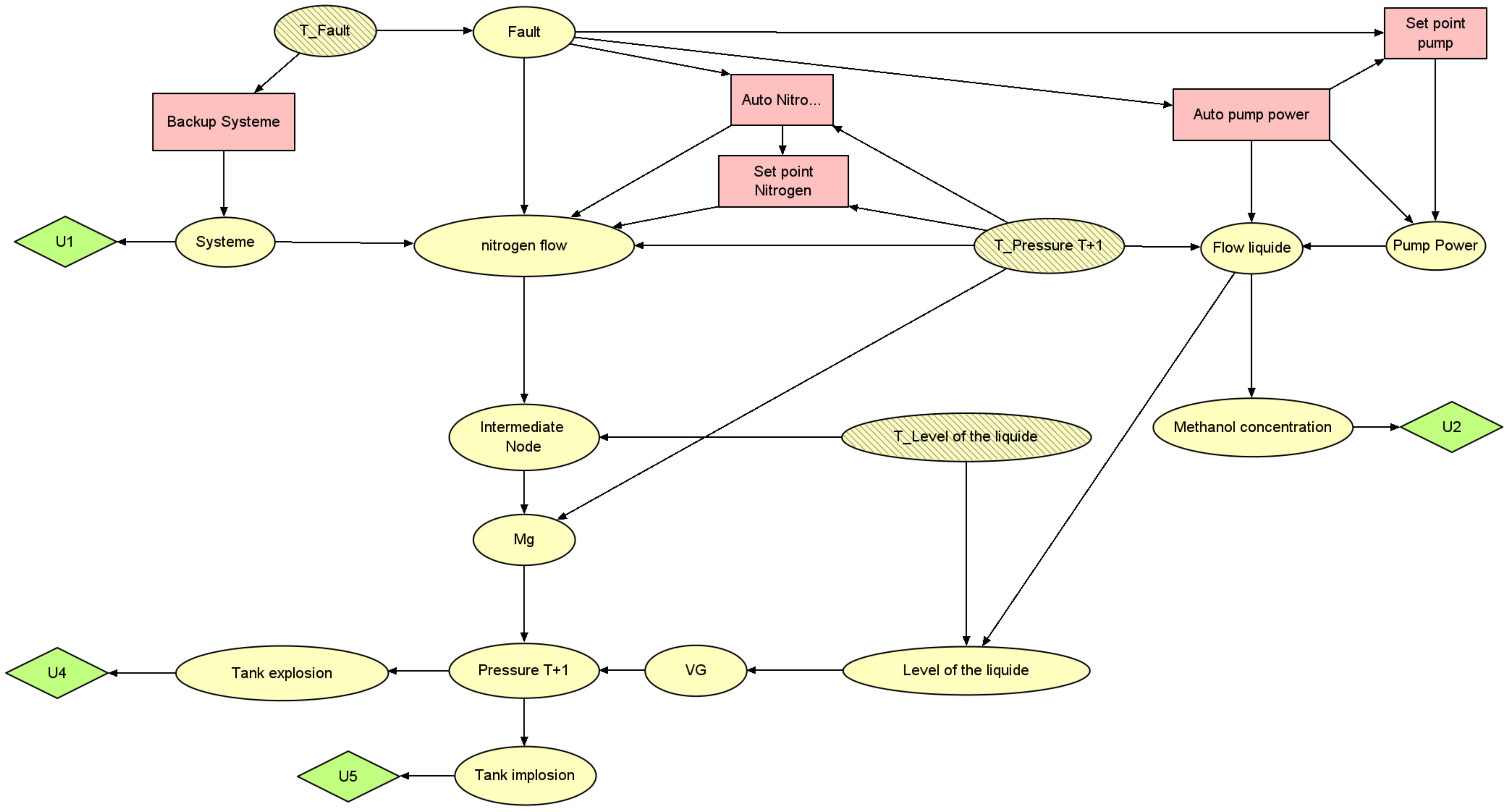
3.1.1. Operational Framework and Objectives of the DID Model

The DID model created for this study is designed to manage the three scenarios outlined in Section 2.2, with an emphasis on the tank system in the process. In the first two scenarios, the DID offers decision support by replicating the physical processes of the tank system, thus assisting operators in achieving systemic equilibrium. The main aim of the model is to regulate the nitrogen injection rate and pump power, preventing the hazards associated with both overpressure (leading to explosion) and underpressure (resulting in implosion). Consequently, the DID aids in maintaining optimal pressure levels inside the tank, vital for the plant’s stability and operational effectiveness.

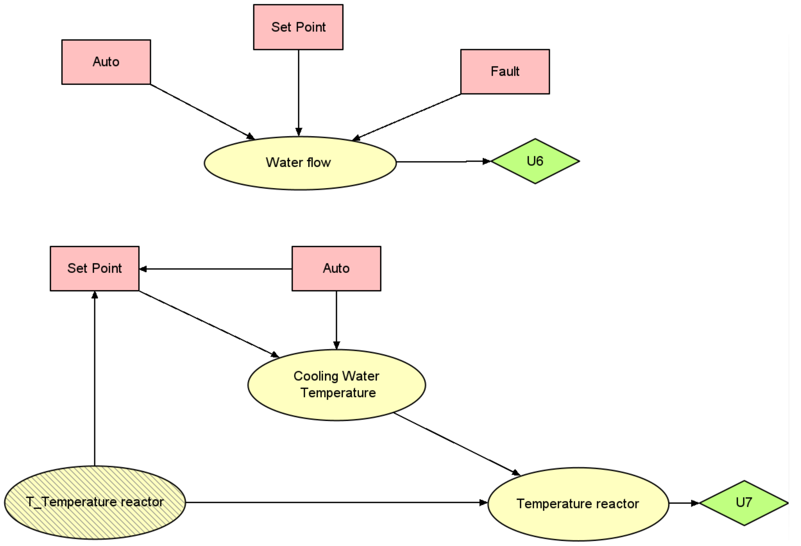
For the third scenario, however, creating a model to represent the entire process was considered infeasible within the scope of this work. Instead, a model was developed to provide decision support specifically for this scenario. Although this more concise model does not capture all aspects of the process, it effectively identifies anomalies and guides the operator in adjusting the process, especially in relation to the reactor’s temperature. This strategy ensures that operators receive precise and applicable advice, enabling them to take suitable measures in response to the scenario without needing a detailed model of the entire system.

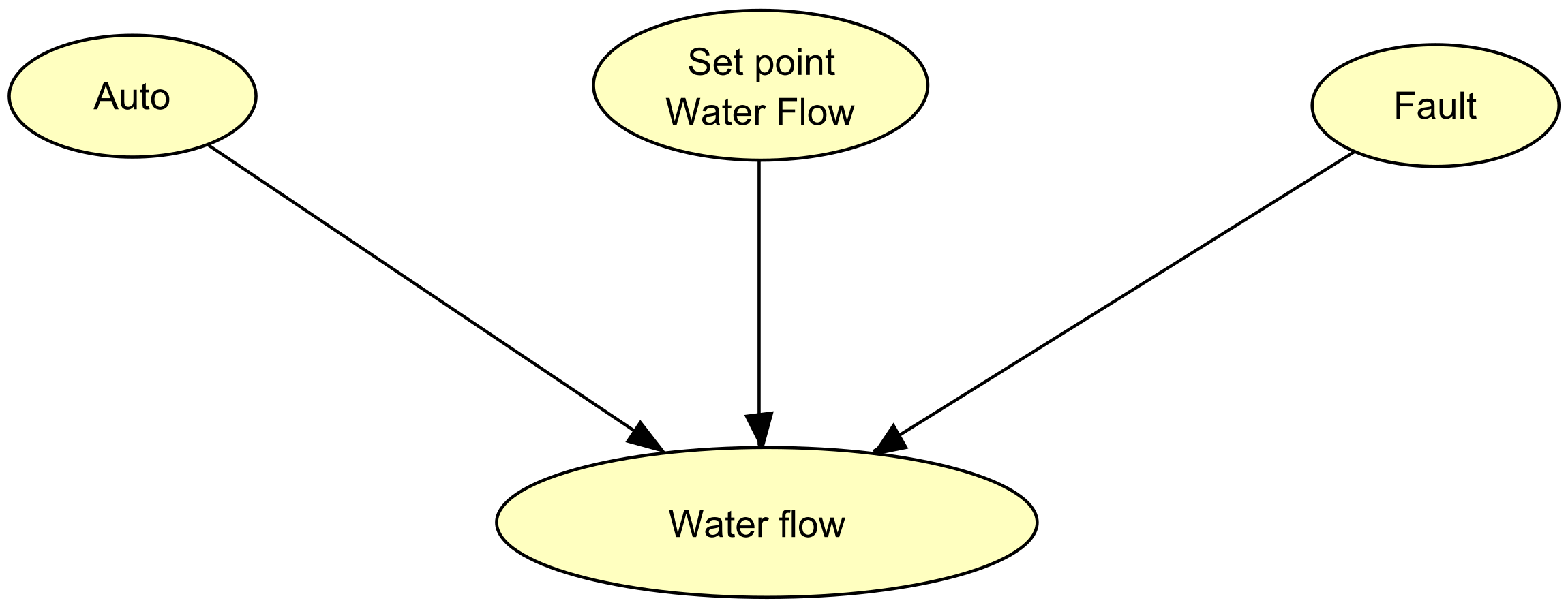
3.1.2. Fault Detection

Fault detection in our system is conducted using conflict analysis, as previously described. The models for fault detection in the first two scenarios and the final scenario are depicted in Figure 9 and Figure 10, respectively. While both models operate on a similar principle, in the first two scenarios, there are additional elements such as the “System” node and “Pressure T+1”. These components reflect the ability to switch to a backup system in scenarios 1 and 2, adjusting the nitrogen flow in response to pressure measurements.

In both models, the default setting is the auto mode with a predetermined flow. A fault is indicated when the actual flow is anomalously low, leading to a conflict between the expected and actual flow readings. To resolve this, the “Fault” node is adjusted to “Fault control”, aligning the low nitrogen flow with the fault condition and thus resolving the conflict. If the issue continues even after reverting to auto mode, a new conflict arises, which is then resolved by adjusting the fault value “Fault valve”.

3.1.3. Parameter and Structure Specification

The specification of parameters in our model is based on the physical equations associated with the process, as detailed in [32], and the model’s inherent logic. Due to the discretization of variables in the model, we adopted a sampling method to create the conditional probability table (CPT). To illustrate this approach, let us consider the calculation of pressure in our case study.

Pressure in our model depends on two variables, Mg (mole) and VG (${\mathrm{m}}^3$), and it follows the perfect gas law:

$$\mathrm{PV}=\mathrm{nRT}$$

(12)

In our experiment, the corresponding physical Equation is

$$\mathrm{P}=\mathrm{Mg}\ast 8.314\ast 1000\ast 298/(28\ast \mathrm{VG})$$

(13)

Here, P is measured in Pascals, Mg in kilograms, and VG in ${\mathrm{m}}^3$. The temperature is set at 298 degrees Celsius, 8.314 J/(mol*K) represents the perfect gas constant, and 28 is the molecular mass of methanol in kg/kmol, converted to kg/mol by dividing by 1000.

The model’s structure is constructed based on this formula, linking Mg and VG to the pressure node. This equation is also used to define the expression in the pressure node, as depicted in Figure 11. Additionally, Mg and VG act as intermediary variables, preventing the direct linking of all variables to the pressure node, which would otherwise create an overly large conditional probability table. This approach also makes the model’s representation of different physical equations more understandable.

For the CPT generation, we employed a sampling method. In our study, we generated 25 values within each interval for the parent nodes Mg and VG. We then calculated the probability of a value falling within the “Pressure T+1” state intervals after applying the relevant formula. This methodology of sampling and probability estimation is similarly applied to other nodes like Mg, VG, level of liquid, flow of liquid, intermediate node, and temperature of the reactor, each governed by their respective physical equations.

The CPTs for “Nitrogen Flow” and “Pump Power” are contingent on the states of their respective parent nodes. For instance, when the system operates in “Auto” mode without any faults, the “Nitrogen Flow” typically maintains a range of approximately 3.9 to 4 ${\mathrm{m}}^3$/h. This range is considered standard for situations where the system autonomously regulates the flow for optimal operation. Similarly, “Pump Power” adjusts according to the states of its parent nodes. These logically structured CPTs enable the Bayesian network to accurately replicate the system’s behavior under various conditions, thereby rendering it an effective tool for decision support and forecasting potential future scenarios.

3.1.4. Utility

In our model, nodes are utilized to represent potential outcomes, such as incidents that could occur within the industrial plant. Upon entering observed values and decisions into the influence diagram, we compute the probabilities of these outcomes. Each outcome, designated as a consequence node, is connected to a utility node that indicates the financial cost associated with that outcome. For instance, the cost of a tank explosion might be estimated at approximately USD 1 million, as referenced in [53]. The probability of such an explosion is influenced by factors like pressure and flow rates, and each decision in the model alters these likelihoods.

The model particularly focuses on outcomes associated with tank pressure, including “Tank explosion” and “Tank implosion”. These outcomes are intricately linked to fluctuations in pressure. For example, the probability of a tank explosion increases proportionally with rising pressure. If the pressure remains within a safe bracket, such as “101,200–102,600” Pa, the risk of explosion is nonexistent. However, if it falls below a critical threshold, like “-inf-96,800” Pa, the risk of explosion becomes inevitable. Conversely, the risk of “Tank implosion” escalates as pressure decreases. This framework assists in predicting and mitigating the risks tied to pressure variations in the tank.

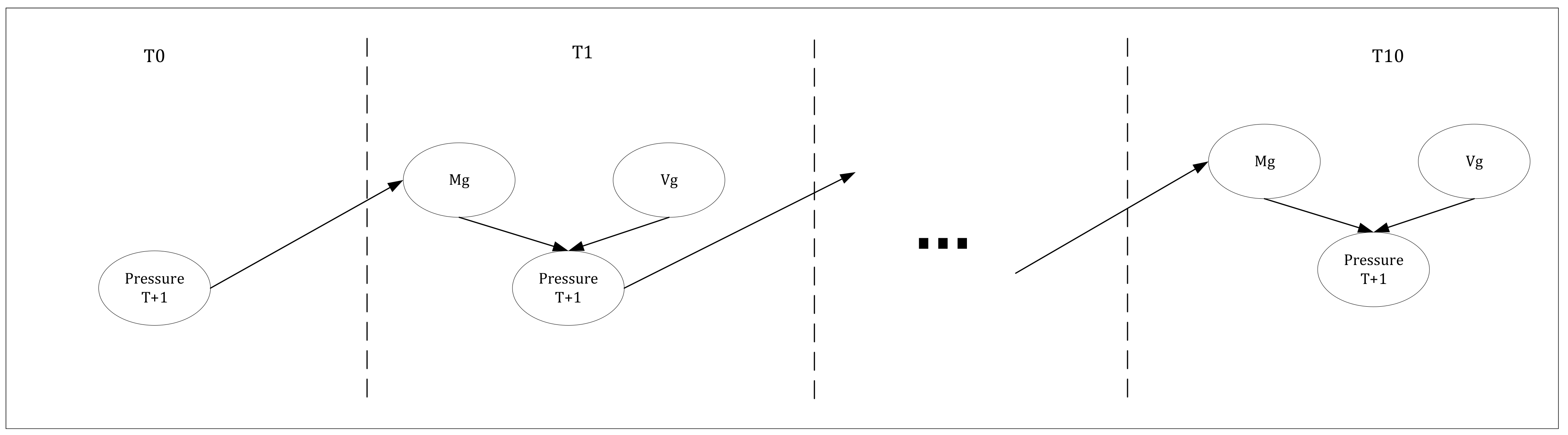
3.1.5. Dynamic Model

In our model, a DID is employed to forecast future states of the system and pinpoint actions that optimize utility at each juncture. This method ensures the selection of optimal actions, taking into consideration both present and forthcoming scenarios. The model functions over 10 time steps, with each representing a one-minute interval. Consequently, it can predict the system’s condition in one-minute segments for the upcoming ten minutes, efficiently capturing the system’s dynamics. This configuration allows us to inform the operator about potential critical events within the next 10 min and recommend the most effective actions to either avert or manage these occurrences.

Decision making within the model is intricately linked to the states of various nodes, such as “Auto” and “Set Point”, which are affected by the current pressure (“Pressure T+1”). This arrangement emulates how an operator would base decisions on both current and anticipated pressure states, thus enhancing the model’s realism and predictive power. The DID is structured to simulate scenarios where the operator makes accurate decisions utilizing these data. Moreover, the model delineates a cause-and-effect relationship between the “Auto” and “Set Point” nodes, wherein the “Auto” mode automatically determines the “Set Point” to a specific value. This aspect is crucial for depicting the system’s reaction to different operational modes and influences the spectrum of potential actions and their consequences. Overall, the model offers an intricate depiction of the decision-making environment, factoring in elements like prevailing conditions, future forecasts, and the interplay between automated and manual controls. This comprehensive methodology renders the DID an invaluable asset for simulating and refining decision making in complex systems.

3.2. AI Framework

In our proposed framework, we combine the predictive capabilities of a DID with the adaptability of RL agents. The DID is precisely constructed based on the physical equations that govern the process, focusing particularly on the dynamics of the tank system and other critical components for specific scenarios. This model is adept at not just capturing the physical dynamics of the tank system but also addressing the inherent uncertainties in the process. It excels in detecting anomalies, representing fault states of the tank, projecting future states, and advising on optimal actions.

A key aspect of a DID is the need for discretizing variables, as influence diagrams are generally more effective with discrete variables. To overcome the challenges posed by discretization, we integrate localized reinforcement learning agents. These agents fine-tune the actions suggested by the DID, offering precise continuous values rather than wide-ranging intervals. This accuracy is crucial in assisting the operator to make more exact decisions. Nevertheless, due to safety considerations, it is essential to exercise caution when incorporating black-box models such as RL agents. Consequently, the continuous value provided by an RL agent is only considered if it aligns with the interval recommended by the DID. If the RL-derived value falls outside this range or seems contradictory, the DID’s suggestion is automatically given precedence. This methodology ensures that the system’s recommendations stay within safe operational limits, harnessing the strengths of both the DID and RL agents to improve decision making while prioritizing safety.

The model operates within a human-in-the-loop (HITL) framework, utilizing a multispecialized reinforcement learning agent (M-SRLA) setup. In this arrangement, multiple agents function independently, and a specific agent is activated to propose the best control strategy to the operator when an abnormality in the process is detected by the influence diagram. This is depicted in Figure 12, sourced from [44]. We refer to this system as “Human-Centered Artificial Intelligence for Safety-Critical Systems” (HAISC), (See Algorithm 1).

Algorithm 1: Influence Diagram-based Recommendation Algorithm.

3.3. Use of the Model

The model’s application for anomaly detection and optimal action recommendation involves a four-step process:

• Initially, the anomaly detection model is utilized to identify potential system faults.
• Subsequently, combining observed data at time T0 with the identified anomaly from step one, various actions at time T1 are evaluated for their maximum utility. This evaluation culminates in devising an optimal action set aimed at either preventing or mitigating potential critical events.
• In instances where an interval-based set point is advised for the operator, a relevant reinforcement learning agent is engaged to refine this value.
• Lastly, the operator is presented with the optimal procedure, delineating the recommended actions based on prior analysis. Additionally, any detected faults and their potential consequences are communicated to the operator.

This systematic method enables comprehensive analysis of the system’s condition, guaranteeing that operators are well-informed about potential complications and possess the most efficacious strategies for their resolution. The integration of anomaly detection, reinforcement learning, and decision-making tools in the model renders it a holistic and potent solution for managing intricate systems. The following illustrates the application of these steps across three scenarios:

Scenario 1.

In the first scenario, a problem is encountered with the nitrogen flow being unexpectedly low, attributed to a malfunction in the automatic control system. This results in pressure levels falling below the normal range. The “Auto” node’s status of “on” contradicts the low nitrogen flow, as auto mode typically ensures a higher flow. Rectifying this discrepancy involves setting the “Fault” node to “control valve failure”. Consequently, the model reflects the system’s current state with this malfunction considered. Analysis suggests that deactivating “Auto” mode and manually adjusting the nitrogen flow’s set point to between 4 and 7 m³/h would yield the highest utility. The reinforcement learning agent, when consulted, suggests a precise value of 5.6 m³/h, aligning with the DID’s recommended range. These actions, along with the set point and fault indication, are then advised to the operator.

Scenario 2.

In the second scenario, a challenge arises with the nitrogen flow, which is noted to be lower than expected. This discrepancy is linked to a malfunction in the primary system’s flow control. Initially, the model cannot determine whether the problem originates from the automatic system or the primary system. The “Auto” node’s status as “on” implies that the nitrogen flow should be higher. A conflict arises between the auto mode and the actual nitrogen flow.

To resolve this issue, the “Fault” node is adjusted to “control valve failure”, thus reconciling the conflict in the model’s initial iteration. However, after a 10 s reevaluation, the problem persists, suggesting a conflict between the expected set point and the actual nitrogen flow. Subsequently, the fault is identified as a “Fault primary system”, leading the model to recommend switching to the backup system. The transition to this system takes two minutes, during which the flow is adjusted to “0–1.5”.

To counter the pressure drop during this period, the model proposes reducing the pump power. This reduction is finely tuned to gradually decrease the pressure drop, ensuring the nitrogen concentration within the system remains unaffected. The optimal set point for the pump power is determined using a reinforcement learning agent in accordance with the DID-suggested interval. Once the pressure is stabilized within the target range, the model advises reverting the pump power to its automatic setting, resuming normal operations. This sequence of actions aims to preserve system functionality while rectifying the fault, thereby minimizing disruptions in the process.

Scenario 3.

In the third scenario, the decision support system identifies a conflict between the “Auto” mode and the water flow in the absorber. Despite following the system’s initial recommendation to switch to manual operation and modify the set point, the issue remains unresolved. A fault is recognized, prompting the system to suggest that the operator should “call supervisor”.

The supervisor’s responsibility in this situation is to acknowledge the problem, which falls outside the purview of control room management, and to dispatch a field operator for direct resolution. Concurrently, the control room operator is directed to focus on monitoring the reactor’s temperature, aiming to prevent any excessive overheating or undercooling.

In the event that the reactor temperature deviates from the norm, the decision support system immediately provides the operator with a specific adjustment for the cooling water system’s temperature. This adjustment is determined using the third reinforcement learning (RL) agent after verifying that the value falls within the range recommended by the DID. Such guidance is vital for keeping the reactor’s temperature within safe operating parameters, thereby ensuring uninterrupted production while the field operator addresses the core problem.

Utilizing this method enables us to leverage a singular model for assessing the current state of the system, projecting future states, and proposing the most suitable procedure for the operator. It is important to underline that these procedures are dynamic and continuously evolving to accommodate changes within the system. This strategy lays a robust groundwork for the development of effective procedures. The procedures provided to the operator through this system are more concise compared to standard procedures, as they concentrate exclusively on necessary actions. Typically, a classical procedure encompasses troubleshooting, action implementation, and monitoring phases. The decision support system serves as an aid in the decision-making process, supplementing but not replacing the existing procedure. It augments the conventional methods by offering tailored recommendations in challenging scenarios. This approach presents a holistic solution, substantially enhancing the decision-making capabilities of operators and, consequently, boosting the overall effectiveness of the system.

4. Experiment

In our experiment, we established two groups: Group 1 (G1), which operated without the aid of the decision support system, and Group 2 (G2), which employed the decision support system. Both groups were exposed to identical scenarios for testing purposes. The objective was to compare their performance and responses, thereby evaluating the effectiveness of the decision support system.

4.1. Participants

Our study involved 48 volunteer participants, predominantly students, who were divided into two groups: 23 in Group 1 and 25 in Group 2. These individuals represented various levels of experience, with a majority being master’s students specializing in chemical engineering. The experimental setup can be seen in Figure 13.

4.2. Situation Awareness

SA in our study is assessed using a bifurcated approach. The first component involves participants completing the situation awareness rating technique (SART) [54,55] questionnaire after each scenario. The SART is a self-assessment instrument designed to evaluate the participant’s awareness of the situation. It focuses on their capabilities to monitor, comprehend, and predict the status of various elements within the environment. The second component of SA assessment occurs in real time during the scenarios through the situation present assessment method (SPAM) [56]. In this method, participants are intermittently asked three specific questions at different stages of the scenario. These queries aim to assess their focus and understanding of the system’s current state, their ability to foresee future states, and their perception of the situation’s complexity and dynamics. This dual methodology facilitates a thorough evaluation of SA by combining reflective self-reporting with immediate, contextual assessments.

The outcomes of the SART questionnaire are illustrated in Figure 14. As indicated by the statistical test in

Table 1. Statistical test results.

	Shapiro–Wilk G1	Shapiro–Wilk G2	Levene’s Test	t-Test	Wilcoxon Rank-Sum Test
Instability	0.43	0.66	0.25	0.19	0.10
Variability	0.07	0.36	0.35	0.66	0.35
Complexity	0.22	0.39	0.63	0.75	0.42
Arousal	0.84	0.28	0.34	0.45	0.16
Spare_capacity	0.67	0.48	0.38	0.60	0.32
Concentration	0.016	0.18	0.58	(0.97)	0.33
Attention_division	0.05	0.96	0.88	(0.99)	0.39
Quantity	0.28	0.29	0.08	0.72	0.36
Quality	0.27	0.28	0.20	0.37	0.22
Familiarity	0.56	0.82	0.10	0.88	0.48

, there is no significant statistical difference in SA between the two groups.

Based on the data in

Table 2. Statistical test results for SPAM index and related factors.

	Shapiro–Wilk G1	Shapiro–Wilk G2	Levene’s Test	t-Test	Wilcoxon Rank-Sum Test
Monitoring	0.00	0.10	0.01	(0.00)	0.00
Planning	0.38	0.36	0.13	0.14	0.09
Intervention	0.07	0.26	0.76	(0.00)	0.00
SPAM_index	0.16	0.61	0.03	0.00	0.00

, and considering that Group G2 consistently registers lower values than Group G1 as shown in Figure 15, the interpretation of the results is as follows:

• Monitoring:

  –

  The Shapiro–Wilk test reveals a non-normal distribution for Group G1 but a normal distribution for Group G2.

  –

  There are significant differences in monitoring, with Group G2 demonstrating lower levels, as indicated by the t-test and the Wilcoxon rank-sum test.

• Planning:

  –

  Both groups show a normal distribution according to the Shapiro–Wilk test.

  –

  There are no notable differences in planning, although Group G2 tends to have marginally lower levels.

• Intervention:

  –

  The Shapiro–Wilk test suggests a non-normal distribution for both groups.

  –

  A significant difference is noted, with Group G2 having a lower score at intervention compared to Group G1.

• SPAM Index:

  –

  The Shapiro–Wilk test indicates a normal distribution for both groups.

  –

  The SPAM index reveals a significant difference, with Group G2 having a lower index than Group G1.

In conclusion, Group G2 consistently demonstrates lower levels of monitoring and intervention and an overall lower SPAM index compared to Group G1. Although no significant difference is observed in planning, Group G2 maintains a trend of lower values across other evaluated aspects Figure 15.

4.3. Workload

The workload of participants was quantitatively evaluated using the NASA Task Load Index (NASA TLX) [57], a broadly acknowledged subjective workload assessment instrument. After each scenario, participants filled out the NASA TLX questionnaire, which assesses six workload dimensions: mental demand, physical demand, temporal demand, performance, effort, and frustration level. The TLX index represents the mean of these dimensions. The bar plot is illustrated in Figure 16, and the statistical analysis is detailed in

Table 3. Statistical test results.

	Shapiro–Wilk G3	Shapiro–Wilk G4	Levene’s Test	t-Test	Wilcoxon Rank-Sum Test
Mental_demand	0.74	0.37	0.52	0.38	0.18
Physical_demand	0.04	0.00	0.20	(0.56)	0.47
Temporal_demand	0.81	0.05	0.28	0.72	0.37
Performance	0.53	0.01	0.05	(0.61)	0.16
Effort	0.54	0.72	0.68	0.85	0.41
Frustration	0.18	0.03	0.83	(0.04)	0.02
TLX_index	0.79	0.63	0.82	0.59	0.21

. Analysis of these findings provides the following insights:

• Mental demand: The analysis reveals no statistically significant difference in mental demand between groups G1 and G2, implying that both groups encountered similar levels of mental workload during the tasks.
• Physical demand: Similarly, the results display no significant difference in physical demand between the groups, suggesting that the physical efforts demanded by the tasks were equivalent for both.
• Temporal demand: Regarding temporal demand, the data show no significant differences, indicating that both groups faced comparable time pressures and constraints while completing the tasks.
• Performance: There was no significant variance in perceived performance among participants from groups G1 and G2, indicating that both groups felt equally effective in their performance.
• Effort: Participant-reported effort levels reveal no significant differences between the two groups, suggesting a parallel level of effort expended in task completion.
• Frustration: A marked difference is noted in frustration levels, with Group G1 experiencing higher frustration than Group G2. This difference implies that the conditions or tools accessible to Group G2 may have helped alleviate frustration.
• TLX Index: The overall TLX Index, a composite measure of workload, exhibits no significant differences between the groups, signifying that the aggregate workload experienced by the participants was uniform across both groups.

In summary, although there are no significant disparities in mental demand, physical demand, temporal demand, performance, and effort between the groups, a marked difference in frustration levels is observed. This implies that while the overall workload may be comparable, the subjective experience of the workload, especially regarding frustration, differs between the groups, with Group G2 (using decision support) experiencing lower frustration levels.

4.4. Performance

This section details a few performance metrics derived from operational data to compare the two groups’ performances. The metrics presented here include reaction time (this is the time it takes to switch the nitrogen valve button from auto to manual depending on the scenario and initial task as written in the procedures); response time (the time it takes to act; for example, in Scenario 1, this means the time it takes to adjust the nitrogen valve scale to the correct value); and overall performance of the operators (this considers the time it takes to recover the low-pressure alarm; in some cases, this includes those who fixed the fault even before an alarm. Those below or equal to the (25th) percentile are grouped as “optimal performance”. Those who fall below or equal to the (50th) percentile are classified as ‘good’, and the rest are classified as “poor performance”). The analysis used data collected from 21 participants in each group ($G1$ and $G2$).

Figure 17 presents a comparison of the overall performance of the groups across the three scenarios.

Table 4. Statistical test for significance between each group for each scenario.

	Wilcoxon Rank-Sum Test
	S1	S2	S3
Reaction time	0.00	0.00	0.14
Response time	0.07	0.00	0.08
Overall performance	0.00	0.05	1.00

provides a comparison for each scenario, focusing on the reaction time and the response time. To determine any significant differences in performance between the groups within each scenario, a nonparametric test, specifically the Mann–Whitney U test ($p<0.05$), was employed.

Based on the overall performance, Group 2 had optimal performance compared to Group 1

Table 5. Time-based performance comparison per scenario.

	Reaction Time		Response Time
	M	SD	M	SD
S1
G1	276.30	46.35	339.30	150.39
G2	106.96	130.96	259.04	170.13
S2
G1	266.91	80.42	361.48	102.57
G2	63.43	84.26	154.83	168.95
S3
G1	190.17	117.22	787.87	207.56
G2	117.38	55.78	680.00	226.43

. This is typically the same for the reaction and response times. The statistical tests Table 4 indicate significant differences in the two groups’ time-based and overall performance metrics while solving the scenarios except in scenario 3, where there is no significant difference between the two groups. One possible interpretation is the wide range of different behaviors inside each group due to the complexity of the task. All in all, the group with the decision support showed better performance than the group without.

4.5. Physiological Data

In this research, a comprehensive quantitative analysis was carried out on physiological metrics gathered using smartwatch technology. Our focus was on three key parameters: heart rate, temperature, and electrodermal activity (EDA) [58]. The aim was to identify significant differences across groups and to uncover underlying patterns and variations within the data. Such insights are invaluable for understanding the physiological responses as captured by the wearable device.

For this analysis, we examined data from Group 1, consisting of 14 participants, and Group 2, with 17 participants. Each participant’s mean values for heart rate, temperature, and EDA were calculated across various scenarios. This approach allows for an assessment and comparison of the mean physiological responses of each group to these scenarios, thereby revealing distinct patterns as monitored by the smartwatch.

The box plot of the different measure men can be seen in Figure 18, Figure 19 and Figure 20.

Table 6. Temperature data comparison.

Comparison	Shapiro–Wilk G1	Shapiro–Wilk G2	Levene’s Test	t-Test	Wilcoxon Rank-Sum Test
Heart rate	0.22	0.18	0.02	0.05	0.09
Temperature	0.46	0	0.98	0.13	0.1
EDA	0	0	0.19	0.17	0.21

details the results of our statistical tests for heart rate, temperature, and electrodermal activity (EDA). For heart rate, both groups G1 and G2 passed the normality test, but a significant difference in variances was identified. The Welch’s T-test revealed a borderline significant difference (p-value = 0.05), corroborated by the Wilcoxon test (p-value = 0.09). Temperature measurements exhibited no significant differences between the two groups. In the case of EDA, neither group demonstrated a normal distribution. The variance differences were not significant, and the Wilcoxon test indicated no significant differences between the groups.

An intriguing observation emerged from the comparative analysis of groups G1 and G2. Group 2 generally exhibited a lower heart rate compared to Group 1. This finding is notable, as it implies that the presence of a decision support system could help reduce stress among control room operators. The inference is that decision support systems might play a vital role in diminishing stress levels, potentially enhancing both the well-being and operational efficacy of operators in high-pressure settings. These results emphasize the significance of incorporating assistive technologies in environments where making decisions under stress is common.

5. Discussion

In this section, we discuss the results presented in this paper. First, we discuss the AI framework built, then the results of the experiment, and finally the limitations of this research.

5.1. The Framework

A significant propriety of utilizing the AI framework is its capability to extract and present a large amount of critical information. This includes indicators of proximity to alarm thresholds, timing of potential events, likelihood, ... . Given that the model represents the process dynamics, it can access and utilize different sources of data. However, it is crucial to balance the amount of information presented to the operator; while the DID framework offers extensive possibilities for data display and analysis, the selection of information to be shown to the operator must be judiciously curated. This careful selection is essential to avoid overwhelming the operator with excessive data, thereby ensuring that the additional information enhances rather than hinders their decision-making process and overall workload management.

Incorporating a “What If” display could be a significant enhancement for operators using a DSS. As suggested in the existing literature [59], this feature would enable operators to visualize the potential consequences of following the actions recommended by the DSS. Such a display can provide a clearer understanding of the implications of different choices, thereby aiding operators in making more informed decisions. The implementation of a “What If” scenario is particularly feasible with the use of dynamic influence diagrams. DIDs can model future states of a system, taking observation and decisions into consideration [39].

One crucial aspect of the DID is the discretization of variables, which influences its precision. Opting for highly precise, fine-grained discretization can lead to an unwieldy model size, resulting in CPTs that are too extensive for practical computation times. Therefore, the choice of discretization must be a balanced one, reflecting the inherent uncertainty in physical measurements while maintaining manageable computation times. Moreover, the dynamic aspect creates easily a high computational time. Future research will be dedicated to optimizing this discretization process and the model, taking into account the uncertainty of physical measurements and the need to control the model’s complexity effectively.

Another critical focus is the meticulous revision of the CPTs for variables not defined by physical equations. This revision aims to ensure that these CPTs, whether based on prior probabilities or logical constructs, more accurately reflect real-world scenarios. This aspect will be thoroughly examined to facilitate a more formal and comprehensive discussion of the CPTs, enhancing the model’s overall reliability and applicability.

Another intriguing aspect of employing DIDs in our study is the potential for integrating data into the model to refine the CPTs, thereby enhancing their alignment with real-world scenarios. While in this study, the model was primarily constructed based on expert knowledge encapsulated in the form of physical equations of the process, the inclusion of empirical data presents a significant opportunity for improvement.

5.2. Experimental Result

Our study reveals that the implementation of a DSS leads to a noticeable reduction in workload for control room operators. This is evidenced by the NASA TLX results, which indicate a significant decrease in frustration levels among operators using the DSS. Additionally, physiological measurements, such as a lower heart rate in the DSS group, further support the notion of reduced workload. In terms of performance metrics like reaction time, response time, and success rates, operators with access to the DSS outperformed those without, aligning with findings in previous studies [16,17]. However, this study also highlights a decrease in SA among operators using the DSS; while the SART questionnaire did not yield significant results, the SPAM methodology revealed a substantial drop in SA for the group with the DSS. This could be attributed to an over-reliance on the DSS, where operators following traditional procedures, despite taking more time, tend to develop a better understanding of the situation.

These findings underscore that while DSSs can significantly enhance the performance of control room operators, they also have the potential to reduce SA. This suggests that DSSs should not be used indiscriminately. Over-reliance on a DSS could undermine the critical role of human operators. The optimal use of a DSS appears to be in situations where operators face constraints, such as time pressure, that prevent them from effectively using traditional procedures. In scenarios where time permits, operators should be encouraged to engage with traditional procedures to gain a deeper understanding of the situation. This balanced approach ensures that the DSS serves as a valuable aid without compromising the essential human element in control room operations.

5.3. Limitations

The framework presented in our study, while innovative and effective, encounters certain limitations that warrant consideration. A technical limitation of our framework is its scalability. Constructing a DID that encompasses the entire process using physical equations is a challenging and time-intensive endeavor. This complexity often necessitates focusing on specific parts of the plant for detailed and accurate modeling. Alternatively, a more generalized model of the process can be developed, but this approach may lead to more generic recommendations, potentially limiting the system’s performance in specific scenarios.

Another limitation lies in the participant demographic of our study. We primarily engaged chemical engineering students who, despite their familiarity with the context, lack real-world experience as control room operators. This gap in practical experience could influence the applicability of our findings to actual industrial settings, where operators may face different challenges and exhibit varying responses to the decision support system.

The physiological data collected during the experiment were analyzed in their raw form, without accounting for individual differences among participants. This approach may overlook the nuances in physiological responses that are unique to each participant. A more detailed and personalized analysis of these data are necessary to gain deeper insights into the physiological impacts of using the decision support system. Such an analysis could provide a more comprehensive understanding of how different individuals respond to the system under various scenarios.

In summary, while our study offers valuable contributions to the field of decision support systems in control room environments, these limitations highlight areas for future research and refinement. Addressing these challenges will enhance the applicability and performance of such systems in real-world industrial settings.

6. Conclusions

In the rapidly evolving industrial sector, control room operators often face overwhelming tasks and alerts, leading to task overload and decision fatigue. This situation, exacerbated by cognitive biases, can compromise decision-making processes. Our research addresses these challenges by introducing an AI-based framework that utilizes dynamic influence diagrams and reinforcement learning to create an effective DSS. This system is designed to assist operators in making swift, well-informed decisions, especially when their own judgment may falter. The framework’s core is a robust, interpretable tool that aids operators during critical process disturbances, combining expert knowledge with a dynamic influence diagram to model uncertainties in complex industrial processes and enhance anomaly detection and action recommendations. The integration of reinforcement learning fine-tunes these recommendations to be more context-specific and precise. This study marks a significant advancement in decision support systems, especially in safety-critical control room environments. We developed a DSS that synergistically combines Bayesian networks’ predictive power with the adaptability of reinforcement learning. This approach models complex systems and uncertainties, improving the adaptability and precision of decision making. The empirical validation of this framework involved a structured experimental study with participants, providing a comprehensive assessment of the system’s impact on operator performance, workload, situation awareness, and physiological responses. The physiological measurements offer an objective assessment of the system’s impact on operators, underlining the importance of empirical testing in understanding the practical application and effectiveness of the DSS. In conclusion, while a DSS can significantly enhance operator performance and reduce cognitive workload in complex industrial environments, it also presents a trade-off with situation awareness. Operators may become overly confident in and reliant on the system, potentially diminishing their situation awareness. Trust emerges as a critical factor in the adoption and effectiveness of a DSS, highlighting the need for a balanced approach in its use. The DSS must be a trusted tool, enhancing decision making without overwhelming operators, and should be employed judiciously, particularly in safety-critical scenarios, to provide crucial guidance and maintain operator engagement and comprehension.