Fault Detection and Location of 35 kV Single-Ended Radial Distribution Network Based on Traveling Wave Detection Method

Abstract

With the progress of society and the iterative improvement of infrastructure construction, the power grid transmission lines have also entered an era of intelligence. The national distribution system has made ensuring the regular operation of the distribution network as well as prompting troubleshooting and detection its top priority. Research on fault diagnosis for 35 kV single-ended radial distribution networks is still in its infancy compared to other hot topics in the industry, such as short-circuit fault detection and fault node localization. This study adopts the 35 kV single-ended radial distribution network as a model, detects fault lines via the traveling wave method, and accurately locates fault nodes using the wavelet conversion method, hoping to quickly identify and locate fault nodes in distribution networks. The experimental results demonstrate that the research method can quickly identify the faulty line and carry out further fault node location detection. The final obtained fault distance is 1.19 km with an actual error of only 0.16 km; the maximum relative errors are only 0.33 km and 0.21 km when the initial phase angle and transition resistance parameters are changed, respectively; and the error amplitude fluctuations are essentially stable. The experimental results also demonstrate that the research method can quickly identify the faulty line and carry out further fault node location.

1. Introduction

As a national infrastructure construction, the distribution network (DN) is not only closely related to the national life, but also plays an important role in the local economic construction, which is one of the important guarantees for the national economic construction and people’s production life [1]. An important concern for the power system is how to ensure the regular operation of the sparger device (SD) and the fast and accurate fault diagnosis of short-circuit failures [2]. The steady-state component approach, the transient component method, the zero-sequence current ratio method, the traveling wave method, and the wavelet conversion method are now the most widely used methods for transmission line (TL) fault identification [3,4]. The traveling wave (TW) method is recognized by the academic community for its simplicity, ease of operation, and accuracy of results [5]. Many scholars have also used machine learning algorithms and artificial intelligence algorithms for the online monitoring and adaptive fault detection of overhead transmission lines [6]. For example, Shu et al. used the existing morphological spectrum fault location technology to establish a position function from the forward and backward fault traveling waves to describe the feature distribution along the fault traveling waves, used the two-dimensional information of the traveling waves to determine the fault location, and verified the feasibility of the proposed method under different fault locations, transition resistance, sampling rate, and fault types [7]. Chen and other researchers proposed a fault location algorithm that can be applied to multi-component power grids. The fault location is determined directly by using the time difference of fault traveling waves measured at substations and branch terminals, and the influence of time error on the positioning accuracy is eliminated by using the quartile method [8]. Although many scholars have proposed effective detection methods, there are very few studies on fault diagnosis in 35 kV single-ended radial SDs. On this basis, this study provides technical support for the rapid response and troubleshooting of fault nodes in power systems.

The study consists of four parts. The first part presents a summary description of the current international research status on SD fault diagnosis and introduces the research methodology. The wavelet conversion method, traveling wave method, and relay protection of the 35 kV transmission network, as well as their respective principles and calculation procedures, are introduced in the second part. The third part is a simulation test of a 35 kV single-ended radiating SD fault diagnosis and the analysis of experimental data. The fourth part is a summary and overview of the experimental results and points out the shortcomings of the study.

2. Related Works

The primary goal of the power system is to quickly and accurately locate the fault node and terminate relay protection when a short circuit fault occurs in the SD. Many academics around the world have conducted extensive research on SD fault detection and have produced various results. Wang and Dehghanian presented an online monitoring system with machine learning analysis to quickly and accurately identify high-impedance faults in power systems to address the power safety issues caused by overhead power line faults under extreme weather conditions. The results of the experiments prove the effectiveness of the system [9]. Biswas and Nayak proposed a unique fault detection and classification strategy based on two criteria; which was demonstrated by comparison with existing methods [10]. Park et al. proposed a circuit fault detection algorithm using Differential Power Processing (DPP) architecture, which simply uses DPP and the inverter’s intrinsic voltage sensor to significantly increase the cost-effectiveness of the PV system. Using a prototype PV system, the circuit fault detection performance was finally confirmed [11]. A fault detection technique based on an adaptively tuned S-transform (ST) was proposed by Li et al. [12]. By including a correction factor in the Gaussian function when computing the ST; the algorithm can extract the high spectrum while retaining the low-spectrum data. The final experimental results support the effectiveness of the method. Rao and Jena eliminated the time synchronization problem by estimating the resistance in TL fault detection using local measurements available on the busbar and comparing the sign of the estimated resistance at both ends of the line segment. The approach can accurately detect closed faults and high-resistance faults in DC microgrids; according to simulation and experimental data [13].

In a grid with a very complicated topology, Zhang et al. developed a TL fault line detection model based on a time series model and a bidirectional GRU (Bi-GRU) model. According to simulation studies, the proposed bidirectional model exhibits superior fault detection performance by reducing the maximum error and not being affected by noise [14]. A fault diagnosis method based on the wavelet transform (WT) analysis of DC side fault characteristics through the grid and frequency domain analysis of DC fault transient cycles has been proposed by Psaras et al. [15]. The method is based on a WT analysis of DC side fault characteristics through the grid while adaptively completing the grid line fault identification. The final experimental data verify the effectiveness of the scheme. According to the modal traveling wave arrival time difference and the fault traveling wave propagation path ratio, Wang and Zhang suggested a fault location principle. The identification of the wave polarity or the calculation of the wave speed values are not necessary for the application of this theory [16]. The wave heights and arrival times were then obtained from the sample data by empirical mode decomposition after preprocessing to ensure that they were all taken from the same frequency range. The validity of the principle was demonstrated by simulation results. A brand-new single-ended measurement hybrid distribution feeder fault segment location identification scheme has been published by Shu et al. [17]. A position function is established from the forward and backward traveling wave components to describe the characteristic distribution of traveling waves along the line, and more accurately locate the actual fault point, using an a priori morphological spectrum-based fault segment identification technique. The experimental results support the effectiveness of the scheme [18].

In summary, many experts and scholars have proposed a variety of effective TL fault detection methods. However, in these research methods, the research results of 35 kV single-ended radiation SD fault line detection are relatively few. Therefore, TW method and wavelet transform method are used in this study to detect and locate the faults of the single-ended radiation equivalent circuit. The purpose of this study is to provide some references for the study of 35 kV single-ended radiation SD faults.

3. Fault Line Detection and Fault Node Location Study of 35 kV Single-Ended Radial SD

In the fault analysis of SD outages, line faults are the primary cause of large-scale outages. The single-phase ground fault, which is also the main indirect cause of other line faults, has the highest probability of occurrence among all the types of SD line faults. The study uses the TW method and the wavelet conversion method to complete the diagnosis of 35 kV single-ended radial SD fault lines and the precise location of fault nodes [19].

3.1. TW Method to Connect Limited Short Circuit Fault Line Detection

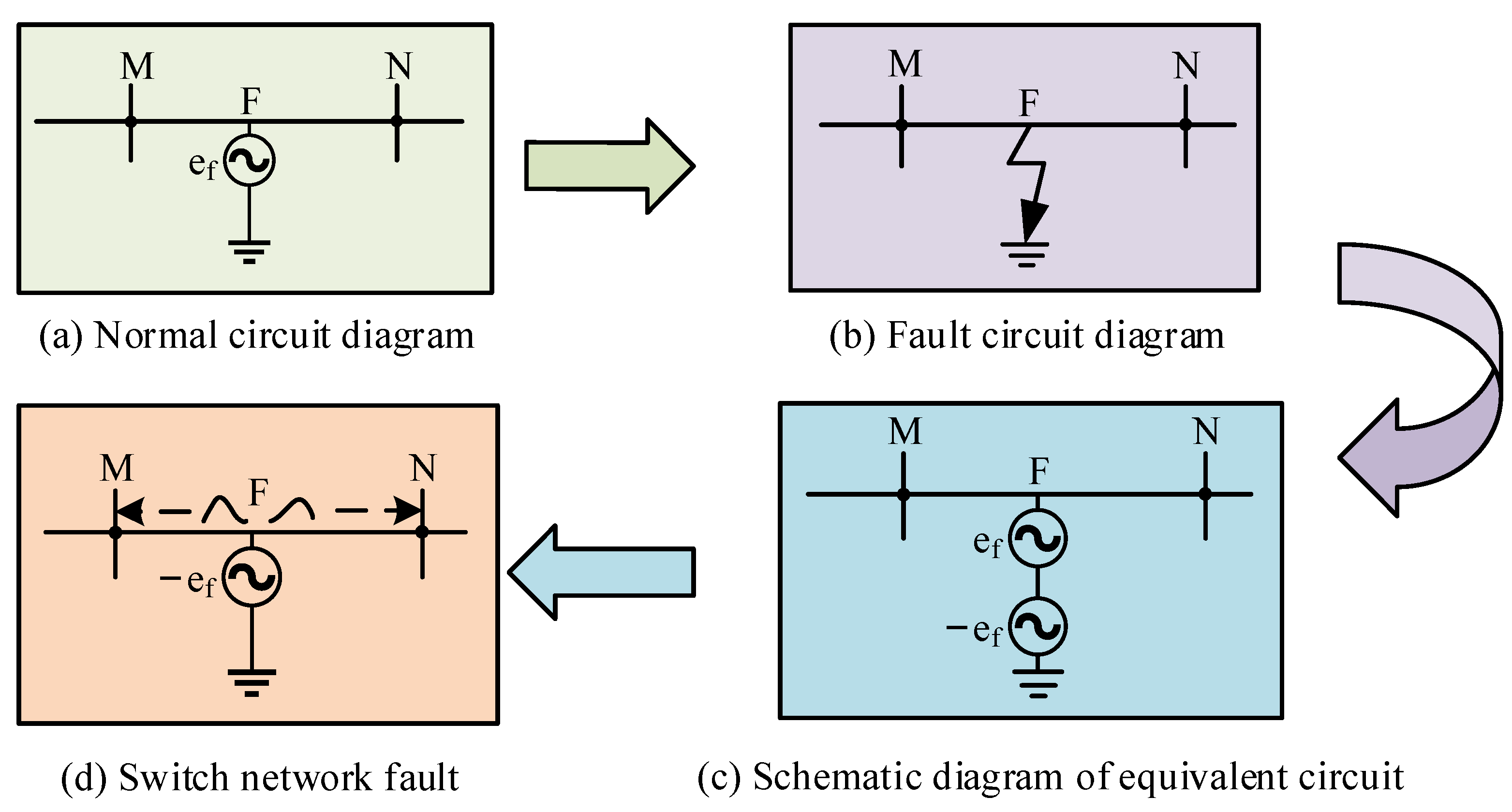
A metallic ground fault on a TL is comparable to the superimposition of a voltage source at the fault location. The voltage produced by the voltage source is equal in magnitude to the normal operating voltage of the line and moves in the opposite direction. The traveling wave approach takes advantage of the traveling wave propagation characteristics to accurately locate the fault node at the time when the fault node begins to generate traveling waves that rapidly propagate through the network. The network detects the traveling wave signal in merely a few seconds because traveling waves travel at speeds close to the speed of light [20]. Figure 1 depicts the schematic diagram (SD) of the entire fault process.

However, in practical situations, TLs are not simple propagation media, and the voltage and current of TLs are continuously changing. In this study, the conductance and capacitance between the wires and the wire resistance and inductance are infinitesimally small. Figure 2 depicts the final model used to determine the distribution parameters of the TL [21].

In Figure 2, $L_0$ is the inductance per unit length, $R_0$ is the resistance per unit length, and $G_0$ is the conductance per unit length. $C_0$ is the capacitance per unit length. At this time, the transmission signal in the TL along the line propagation change function, that is, the TL propagation constant $\gamma$, is revealed as Equation (1):

$$\gamma =\sqrt{(R+j\omega L)(G+j\omega C)}=\alpha +j\beta$$

(1)

In Equation (1), $\omega$ is the frequency of the transmitted signal, $C$ is the line capacitance, $L$ is the line inductance, $\alpha$ is the attenuation coefficient of the TL, reflecting the energy loss of the signal during propagation, and $\beta$ is the phase shift coefficient of the TL. According to Kirchhoff’s law, i.e., KVL equation and KCL equation to form a set of differential equations, Equation (2) displays the expression for the collection of equations:

$$\{\begin{array}{l}-\frac{\partial u}{\partial x}=Ri+L\frac{\partial i}{\partial t}\\ -\frac{\partial i}{\partial x}=Gi+C\frac{\partial u}{\partial t}\end{array}$$

(2)

In Equation (2), $Ri$ is the nodal resistance and $Gi$ is the nodal conductance. Further solving Equation (2) yields the equations, and the expressions of the equations are as in Equation (3):

$$\{\begin{array}{l}U(x)=A_1{e}^{-\gamma x}+A_2{e}^{\gamma x}\\ I(x)=\frac{1}{Z_0}(A_1{e}^{-\gamma x}-A_2{e}^{\gamma x})\end{array}$$

(3)

In Equation (3), $U(x)$ represents the voltage traveling wave (VTW), $I(x)$ represents the current TW (CTW) in the TL, $A_1$ is the initial amplitude of the TW, and $A_2$ is the changing amplitude of the TW. $Z_0$ is the characteristic impedance, which is expressed in Equation (4):

$$Z_0=\sqrt{\frac{R+j\omega L}{G+j\omega C}}$$

(4)

Solving Equation (3) in the complex domain, it lets $A_1=\left|A_1\right|e^{j{\varphi }_1}$, $A_2=\left|A_2\right|e^{j{\varphi }_2}$, and converting the complex vector into the form of a time function results in the time domain expression of the TW. Equation (5) is used to compute the VTW’s time domain expression:

$$u(x,t)=\sqrt{2}\left|A_1\right|e^{-\alpha x}\cos (\omega t-\beta x+{\phi }_1)+\sqrt{2}\left|A_2\right|e^{-\alpha x}\cos (\omega t+\beta x+{\phi }_2)$$

(5)

In a similar manner, Equation (6) can be used to generate the time domain expression of the CTW:

$$i(x,t)=\sqrt{2}\frac{\left|A_1\right|}{Z_0}{e}^{-\alpha x}\cos (\omega t-\beta x+{\phi }_1)+\sqrt{2}\frac{\left|A_2\right|}{Z_0}{e}^{-\alpha x}\cos (\omega t+\beta x+{\phi }_2)$$

(6)

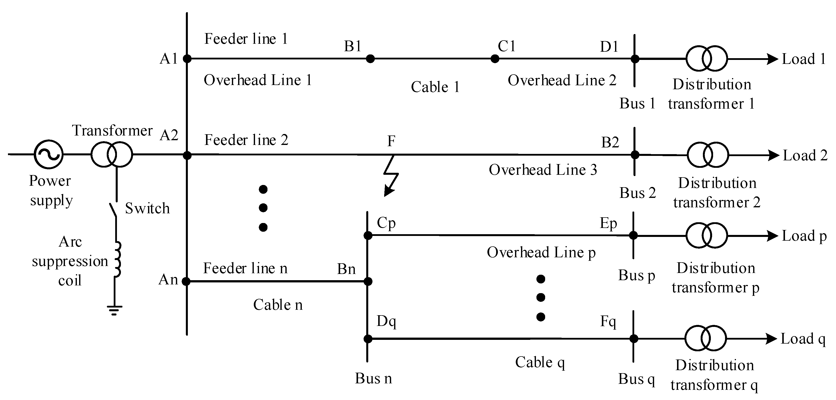
From Equation (6), when a fault occurs, the line wave amplitude change decays exponentially as an attenuation coefficient $\alpha$ and the phase changes as a function of the phase coefficient $\beta$. Figure 3 schematically depicts the topology of the single-ended radial SD model.

As shown in Figure 3, in order to simplify the line, it is assumed that the line used wires that are the same type as the TL, that is, the same TL wave impedance was used on the line. The final obtained voltage and electropop wave amplitude relationship are expressed in Formula (7).

$$\{\begin{array}{l}{u}_A=\frac{2}{n}{u}_F\\ i_F=-\frac{2(n-1)}{n}\frac{u_F}{z}\\ i_N=\frac{2}{n}\frac{u_F}{z}\end{array}$$

(7)

In the Formula (7), the bus endpoint VTW is represented by $u_A$; the fault line endpoint CTW is represented by $i_F$; the TL wave impedance is represented by $z$; the non-fault line endpoint CTW is represented by $i_N$; and the fault initial VTW is represented by $u_F$; $n$ is for the number of feeders.

3.2. Research on Methods for Locating Faulty Nodes

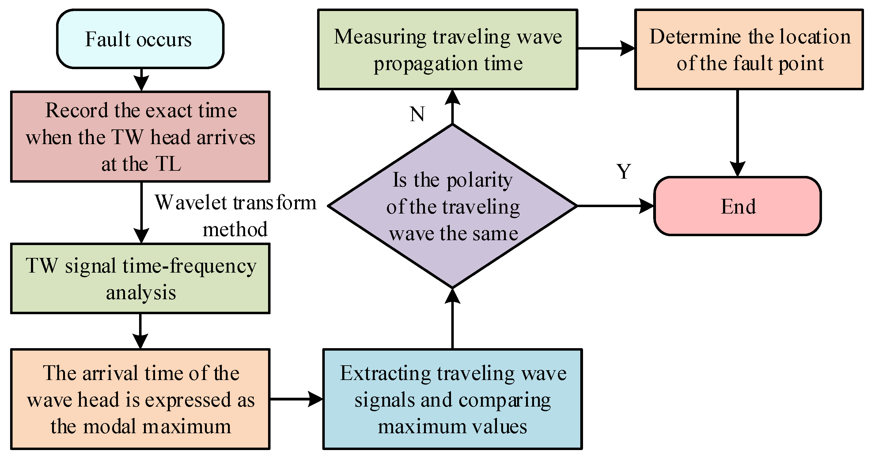
After confirming the fault line, the time difference between the arrival of the line mode VTW (LM) and the zero mode VTW (ZM) at the monitoring point can be used to determine whether the fault occurred in the first or second half of the fault line, and the exact fault distance can be calculated from the arrival moments of the first two wavefronts [22,23]. Figure 4 shows the flowchart of a single-ended radial network fault location.

In the event of a problem, the exact minute the TW head arrives at the TL must be recorded. The time–frequency analysis of the TW signal is performed using the WT method to explain both the local characteristics of the signal in the time–frequency domain and the overall picture of the signal. In order to accurately enhance the sudden change characteristics of the TW signal, the WT method is used to refine the TW signal through the operation functions of scaling and translation, and to express the arrival time of the wavehead as the modal maximum. Firstly, a wavelet basis function $\phi (t)$ is set up, and then, $\phi (t)$ should satisfy the relation as Equation (8):

$$\{\begin{array}{l}\phi (t)\in L^2(R)\\ {\displaystyle {\int }_{-\infty }^{+\infty }\frac{{\left|\phi (\omega )\right|}^2}{\omega }}d\omega <+\infty \end{array}$$

(8)

In Equation (8), $L$ is the line inductance, and by performing a series of scaling and translation of $\phi (t)$, the expression of the continuous wavelet basis function ${\phi }_{b,a}(t)$ is obtained as in Equation (9):

$${\phi }_{b,a}(t)=(\frac{-b+t}{a})a^{-\frac{1}{2}}\phi , a>0, b\in R$$

(9)

In Equation (9), $a$ is the scale factor, which is related to the stretching and compression of $\phi (t)$, and $b$ is the translation factor, which is related to the translation of $\phi (t)$ in time. The duration of the transient signal at high frequency is too short and the scale factor $a$ needs to be reduced to improve the time resolution. For low-frequency steady-state signals with a slow frequency change, the scale factor $a$ should be increased to improve the frequency analysis rate. Function $f(t)\in L^2(R)$ is revealed in Equation (10):

$$W_f(b,a)=(f(t),{\phi }_{a,b}(t))={\left|a\right|}^{-\frac{1}{2}}{\displaystyle {\int }_{-\infty }^{+\infty }f(t)}\phi (\overline{\frac{t-b}{a}})dt$$

(10)

In Equation (10), $\overline{\frac{t-b}{a}}$ denotes the conjugate of $\frac{t-b}{a}$. Considering that the scale factor $a$ and the translation factor $b$ as continuous variables involved in the continuous WT would generate a huge amount of computation, the study discretizes the wavelet basis function. Equation (11) illustrates the formulation of the wavelet basis function following the discretization process:

$${\phi }_{j,k}(t)=2^{-\frac{j}{2}}\phi (2^{j}t-k)$$

(11)

Equation (11) can be interpreted as the family of functions ${\phi }_{j,k}(t)$ obtained by scaling $\phi (t)$ by a factor of $2^j$ and translating $k$ into $\left\{{\phi }_{j,k}(t)\right\}, j ,k\in Z$. The discrete WT of the function $f(t)\in L^2(R)$ results in the expression in Equation (12):

$$W_f(j,k)=(f(t),{\phi }_{j,k}(t))$$

(12)

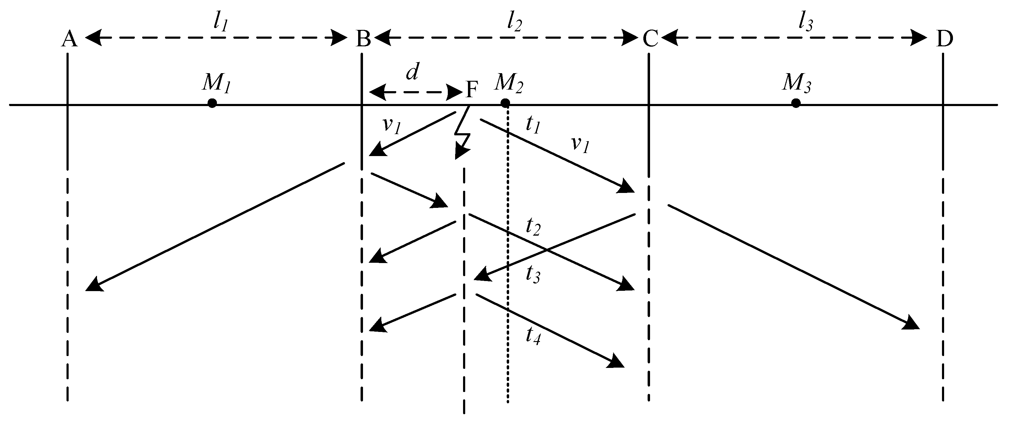
In order to facilitate the calculation, an equivalent circuit was built and measurement devices were placed in the line to measure the change in VTWs in each line. Figure 5 displays the final diagram of the TL [24].

In Figure 5, $M_1$, $M_2$, and $M_3$ are the VTW measurement devices at the midpoint of the line, $F$ is the fault node, $d$ is the fault distance, and $v_1$ is the TW transmission speed. Taking the measurement point at $M_2$ as an example, the arrival time of the TW head measured here is recorded as $t_1$, $t_2$, $t_3$, and $t_4$, respectively, and the initial TW propagation relation is finally obtained as Equation (13):

$$\{\begin{array}{l}\frac{1}{2}{l}_2-d=v_1{t}_1\\ d+\frac{1}{2}{l}_2=v_1{t}_2\\ \frac{1}{2}{l}_2-d+l_2=v_1{t}_3\end{array}$$

(13)

In Equation (13), $l_2$ is the length of the bus $BC$, $t_1$ is the time of the initial TW propagation to the measurement point $M_2$, $t_2$ is the time of the initial TW reflected by the bus $B$ and then refracted by the fault point $F$ to finally propagate to the measurement point $M_2$, and $t_3$ is the time of the initial TW propagation to the bus $C$ and reflected back to the measurement point $M_2$. Equation (13) is calculated to obtain the time expression of the initial TW head arriving at the measurement point $M_2$ as Equation (14):

$$\{\begin{array}{l}{t}_1=\frac{l_2-2d}{2v_1}\\ t_2=\frac{l_2+2d}{2v_1}\\ t_3=\frac{3l_2-2d}{2v_1}\end{array}$$

(14)

Equation (14) compares $t_1$, $t_2$, $t_3$, and finally $t_1<t_2<t_3$, so it can be determined that $t_1$ is the first wavehead arrival time detected by $M_2$ and $t_2$ is the second wavehead arrival time detected by $M_2$. The final equation for the fault distance $d$ is given in Equation (15):

$$d=\frac{(t_2-t_1)v_1}{2}$$

(15)

3.3. 35 kV TL Relay Protection

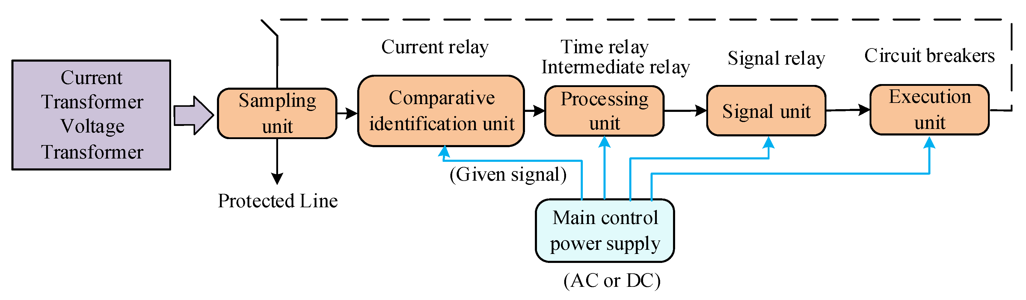
In practice, a good relay protection can not only respond to unexpected situations in time to avoid the further expansion of the accident scale, but also isolate and mark the fault nodes in a timely and effective manner, providing a great boost to the progress of subsequent restoration work [25]. The power system relay protection device is an automatic device used to carry out line faults and abnormal situations in which the circuit breaker trips and issues warning signals. When a fault or abnormal condition occurs in the power system, the relay protection device can be used to indicate the first time to investigate the fault line and take shutdown measures for the fault node to prevent further expansion of the fault. At the same time, it can issue warning signals, report abnormal data information, and help maintenance personnel eliminate abnormal conditions. This protects the TL and minimizes outage losses. Figure 6 displays the SD of the relay protection device [26].

The relay protection for 35 kV TLs must meet the performance standards of high sensitivity, fast response, safety, and reliability in order to meet the daily maintenance and regular operation of 35 kV TLs. This requires that the relay protection device correctly distinguishes the operating state of the protected components and ensures that no misoperation occurs during a normal operation of the TL.

The common relay protection measures used in SD fault handling are two-stage differential protection and multi-stage differential protection. Two-stage polar differential protection uses the load mode for relay protection on the trunk feeder [27]. If a fault occurs on a full overhead feeder rather than a full cable feeder, it is important to quickly disconnect the current at the fault location in order to diagnose whether the fault is transient or permanent. This determination depends on whether the circuit breaker was successfully reset, as well as the branch, the node, and whether or not the branch is an overhead line, where the fault actually occurs.

The multi-level differential protection is to set the corresponding time-delayed protective action on the substation outlet switch, i.e., recloser, and to design the main feeder switch with the help of voltage time-type segmentation equipment, while increasing the protective action delay time and fast reclosing equipment, and to complete the relay protection of the whole TL by the online monitoring of each part of the circuit parameter index and monitoring of the plant equipment status.

4. Simulation Model Fault Detection and Precise Positioning Verification Analysis

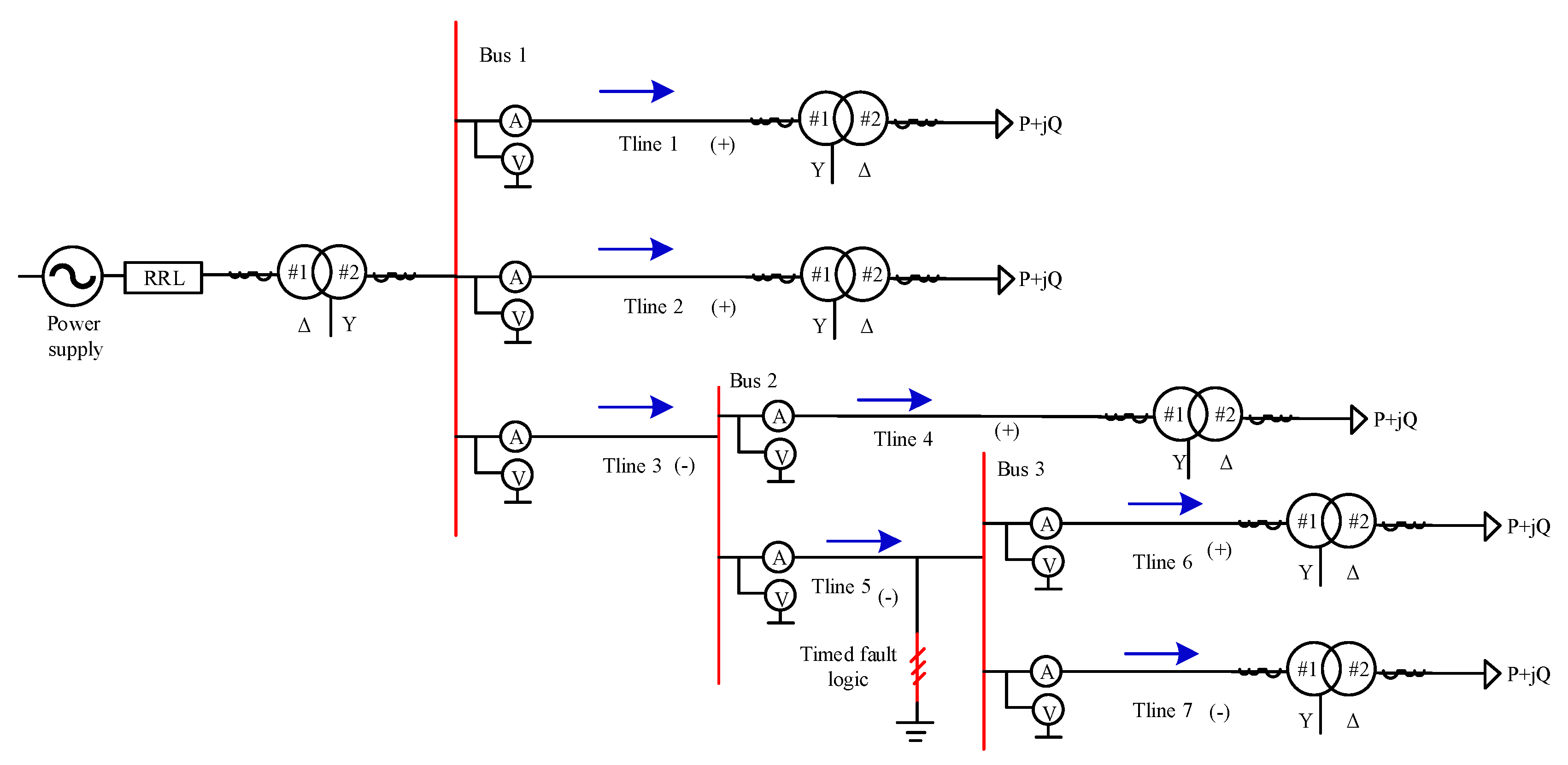
A 35 kV single-ended radial SD LDl is created in the PSCAD/EMTDC power system simulation program for simulation verification in order to assess the viability of the study methodology. The Bergeron model is chosen for the LDl, and the lines selected are all homogeneous lines with the same wave impedance. A measuring device is placed at the beginning of each line to measure the VTW and CTWs of each line. The input end uses a Δ-Y 110/35 kV transformer with a rated capacity of 31.5 MVA, and the output end is connected to a Y-Δ 35/10 kV transformer with a capacity of 1 MVA. The load model is an inductive fixed load, and the input and output transformers are operated without grounding the neutral point. Figure 7 displays the schematic of the 35 kV single-ended radial SD simulation model.

The blue arrows in Figure 7 indicate the direction of the propagation of the TW in the TL, and $p+jQ$ indicates the power supplied by line $S$. The figure’s positive and negative signs for each line of the VTW and CTW LD components of the modal maximum product $S_N$ of the positive and negative can be seen in line 3; and in line 5 modal maximum product $S_N$ for the negative sign, the rest of the line modal maximum product $S_N$ are positive. 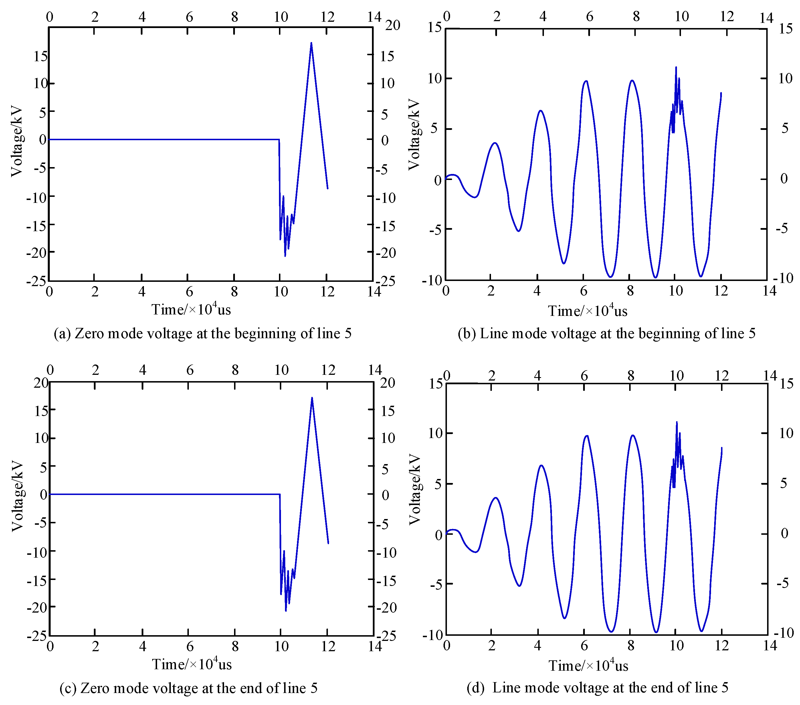Line 3 and line 5 are suspected fault lines; further observation found that the end of line 3, which is connected to line 5 product $S_N$, is negative, while the end of line 5, which is connected to line 6 and line 7 product $S_N$, are positive, thus confirming that line 5 is a fault line. The measured TW signals from each instrument device were decoupled into ZM and LD TW signals using the Carrenbauer transform, and the waveforms are shown in Figure 8.

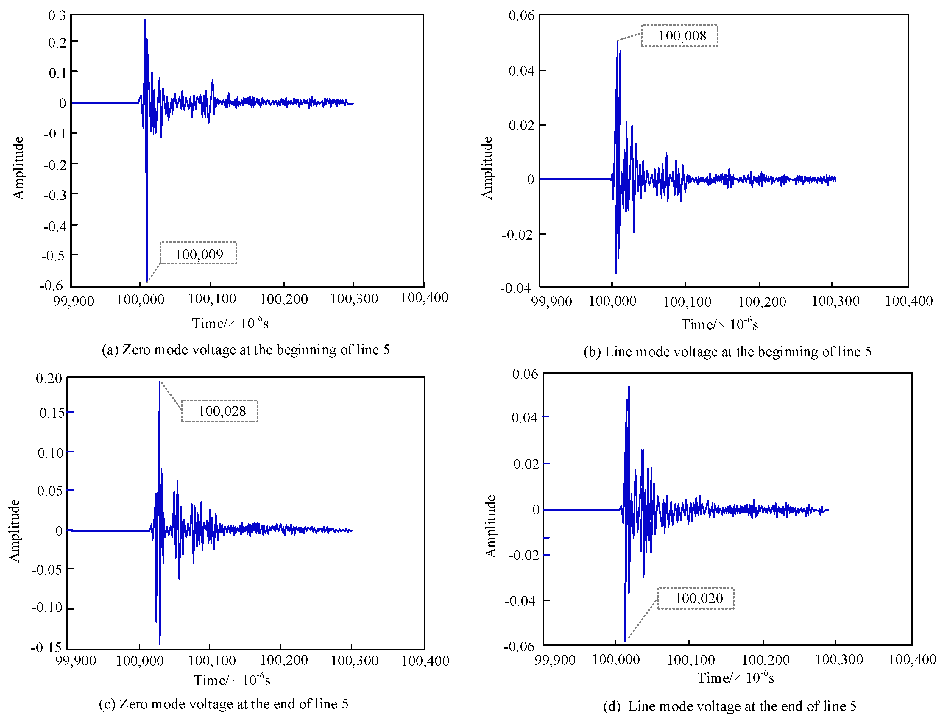
Due to the extremely small changes in ZM voltage and LD voltage at the first and last ends of the fault line, the waveform direction is almost the same on the TWform diagram, and it is not possible to obtain accurate data visually on the TWform diagram. Next, the four groups of TWform signals are WTed separately. The WT diagram is shown in Figure 9.

According to Figure 9, the WTed waveform is very dense, whereby the first wavehead characteristics are clear and obvious, and finding the first wavehead arrival moment can be very direct and accurate. Combined with the data in Figure 9, it can be seen that line 5 first exhibits initial TW arrival moments of 100,009 × 10⁻⁶ s and 100,008 × 10⁻⁶ s for a ZM voltage and an LD voltage, respectively; and then ends with initial TW arrival moments of 100,028 × 10⁻⁶ s and 100,020 × 10⁻⁶ s for a ZM voltage and an LD voltage, respectively. Further calculation is required to obtain the line with the first measured modal time difference of 1 × 10⁻⁶ s, as well as the line that ends with a modal time difference of 8 × 10 s. The modal time difference measured at the end of the line is 8 × 10⁻⁶ s. It is found that the fault occurred in the first half of line 5 since the modal time difference at the beginning of the line is negligible. The LD voltage waveform and WT are shown in Figure 10 after measuring the first two waveheads of the LD component of the voltage at the center and WTed.

According to the data in Figure 10b, we can determine the arrival moment of the first wavehead as 100,010 × 10⁻⁶ s, and the arrival moment of the second wavehead as 100,018 × 10⁻⁶ s. Substituting the data into Equation (15), we can determine the fault distance $d$ as 1.19 km. In summary, we can determine the fault prediction result as the fault occuring in line 5, 1.19 km away from the bus, which is 0.16 km from the actual error.

The study sets up simulation tests to confirm the accuracy of the study scheme for various transition resistance instances since it is assumed that the transition resistance following the fault will have some impact on the amplitude of the initial TW of the fault. The study generates a single-phase ground fault on line 5 with a fault start phase angle of 60 degrees, a fault onset time of 0.1 s, and a fault duration of 0.02 s in the 35 kV single-ended radial SD simulation model shown in Figure 7.

Table 1. Fault diagnosis results under different fault resistances.

Fault Distance Distance Busbar 2	Transition Resistance (Ω)	Fault Section	Positioning Results (km)	Relative Error (km)
0.88 km	10	First half	1.09	0.21
	50	First half	1.07	0.19
	100	First half	1.02	0.14
2.64 km	10	First half	2.77	0.13
	50	First half	2.51	0.13
	100	First half	2.49	0.15
4.72 km	10	The second half	4.88	0.16
	50	The second half	4.51	0.21
	100	The second half	4.93	0.21

shows the final data results after varying the transition resistances and distances from the fault point to bus 2.

The localization results are still very accurate, with a maximum relative error of only 0.21 km for control experiments with fault distances of 0.88 km, 2.64 km, and 4.72 km, respectively. The magnitude of the relative error also does not change significantly with the 5-fold and 10-fold amplification of the junction resistance, with a maximum relative error change of only 0.08. This further demonstrates the accuracy and stability of the method by excluding the effect of fault distance, transition resistance, and fault distance on the precise location of faults in the transmission network.

In order to test whether the research method is applicable to different fault initial phase angles, a single-phase ground fault is set up on line 5 along the simulation model shown in Figure 7 to continue the control experiment. The fault transition resistance is set to 10 Ω, the start time of the fault is 0.1 s, the duration of the fault is 0.02 s, and diffraction measurements are set up to measure the voltage drop on the line.

The statistics in

Table 2. Fault diagnosis results under different initial phase angles.

Fault Distance Distance Busbar 2	Fault Initial Phase Angle (°)	Fault Section	Positioning Results (km)	Relative Error (km)
0.88 km	30	First half	1.13	0.25
	60	First half	1.06	0.18
	90	First half	1.21	0.33
2.64 km	30	First half	2.81	0.17
	60	First half	2.79	0.15
	90	First half	2.41	0.23
4.72 km	30	The second half	4.51	0.21
	60	The second half	4.57	0.15
	90	The second half	4.91	0.19

show that the largest relative error is only 0.33 km, and that changing the initial phase angle has little to no effect on the accuracy of the method. The variation in error is minimal when the initial phase angle is changed, with a maximum relative error variation of about 0.18. It also confirms that the research method has good robustness and can correctly find the fault locations in the transmission network despite changes in the initial phase angle and transition resistance, demonstrating its viability and superior performance.

5. Conclusions

The study employed the TW method to identify problematic lines and the WTation approach to determine the exact location of faulty nodes in 35 kV single-ended radial SDs. The experimental results demonstrate that the faulty node is located in the first half of the line since the modal time differences between the first and second ends of the faulty line are 1 × 10⁻⁶ s and 8 × 10⁻⁶ s, respectively. The arrival times of the first wavehead and the second wavehead are 100,010 × 10⁻⁶ s and 100,018 × 10⁻⁶ s, respectively, according to the wavelet transform of the LD TW at the center. The final fault distance $d$ is 1.19 km, and the error with the actual data is 0.16 km, which meets the experimental requirements. The maximum relative error is only 0.33 km and 0.21 km with a minimal fluctuation of the error magnitude, which proves the accuracy and stability of the algorithm and its good robustness. This study has carried out in-depth research on the distribution network fault location measurement point layout, the factors affecting the positioning accuracy, the initial fault traveling wavehead calibration and the test effect, and achieved a series of research results. However, our work still has a long way in order to achieve a high-precision fault location of the distribution network. Because the proposed fault traveling wave initial head calibration algorithm is still an improvement on the traditional local feature method, it is easy to be disturbed by noise and other influencing factors. With the deepening of the research on artificial intelligence algorithms such as deep neural network, its application in the field of distribution network fault location is also a future research direction.