
Comprehensive Evaluation Index System and Application of Low-Carbon Resilience of Power Grid Containing Phase-Shifting Transformer under Ice Disaster
Abstract
:1. Introduction
- (1)
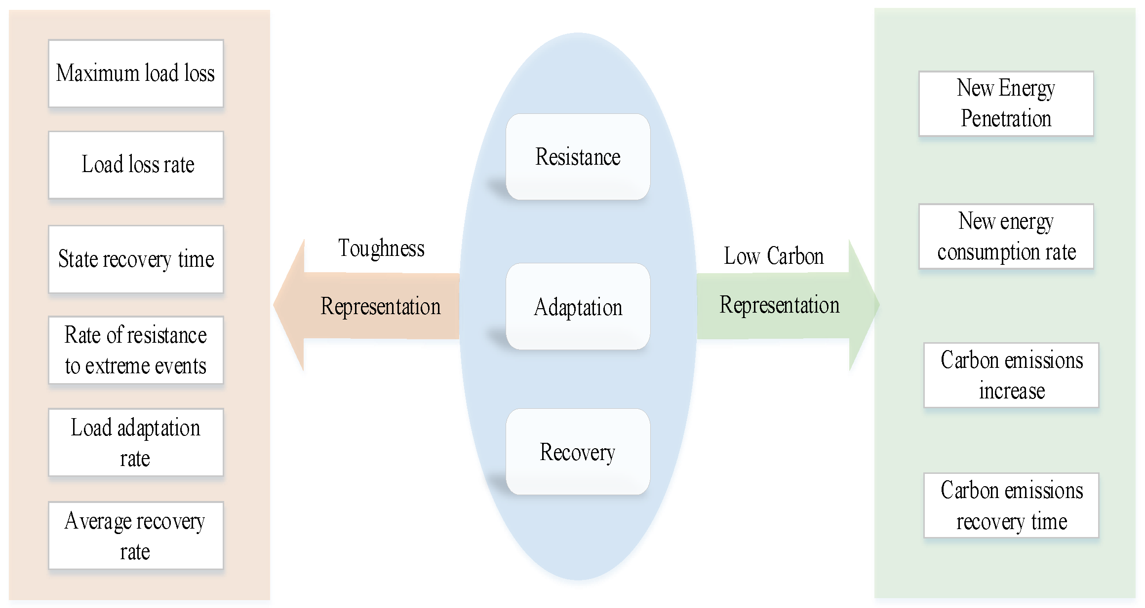
- According to the concept of low-carbon resilience (LCR), the evaluation index of low-carbon toughness is put forward. Compared with the traditional single resilience evaluation index, the LCR level of power grids under extreme disasters is measured from two new angles of carbon emission change and carbon emission recovery time.
- (2)
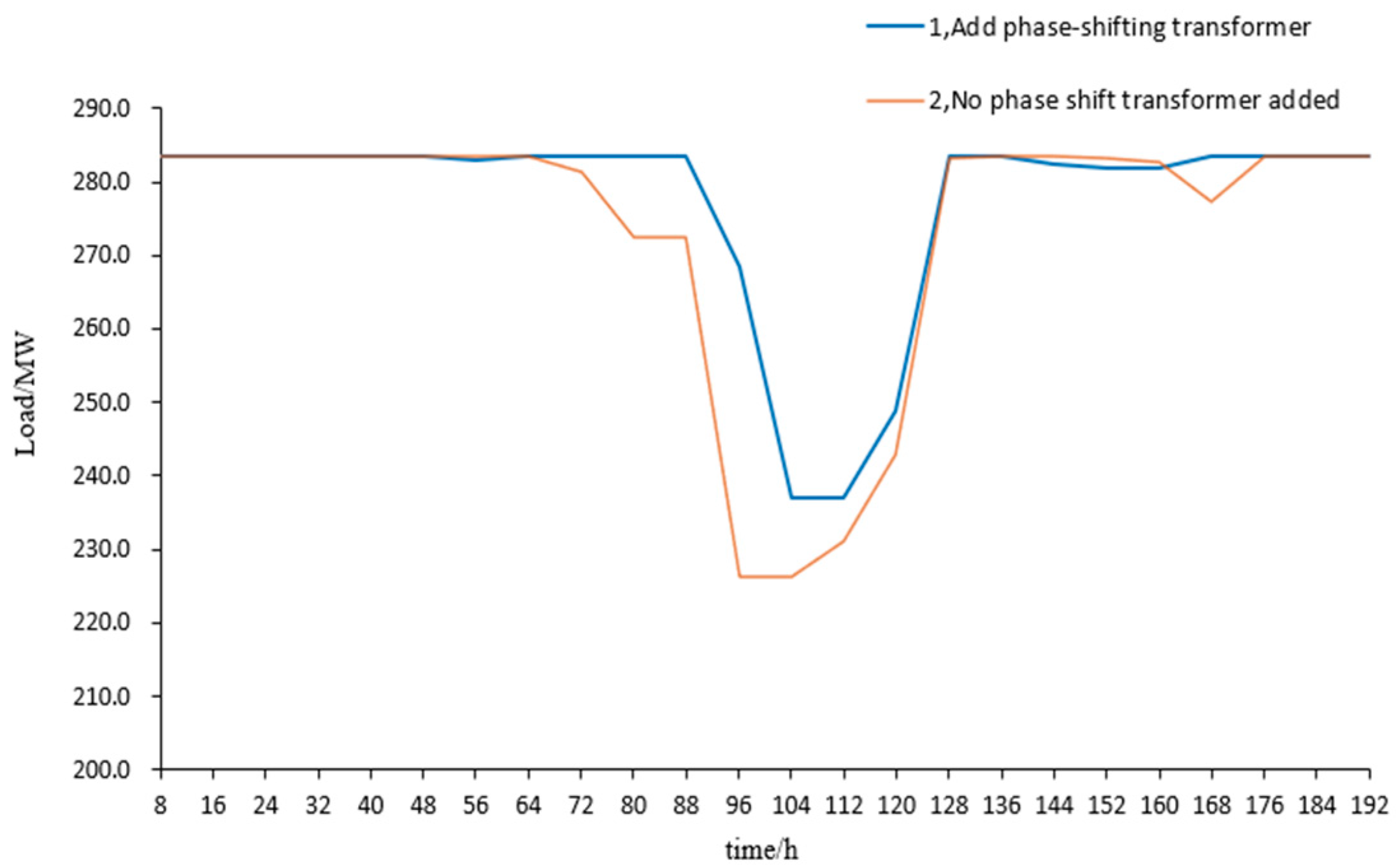
- Considering the equivalent model of the branch with the phase-shifter transformer, the power flow distribution of the line is adjusted through the power regulation of the phase-shifter transformer so as to improve the transmission capacity of the power grid.
- (3)
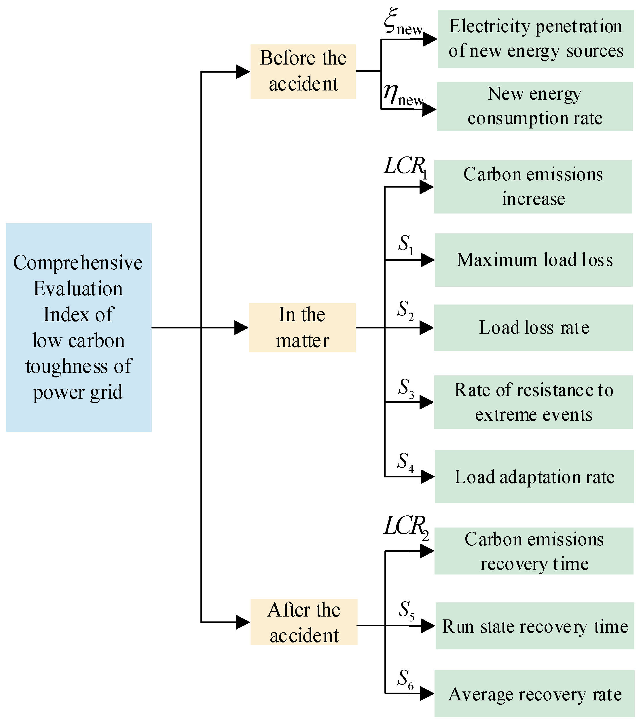
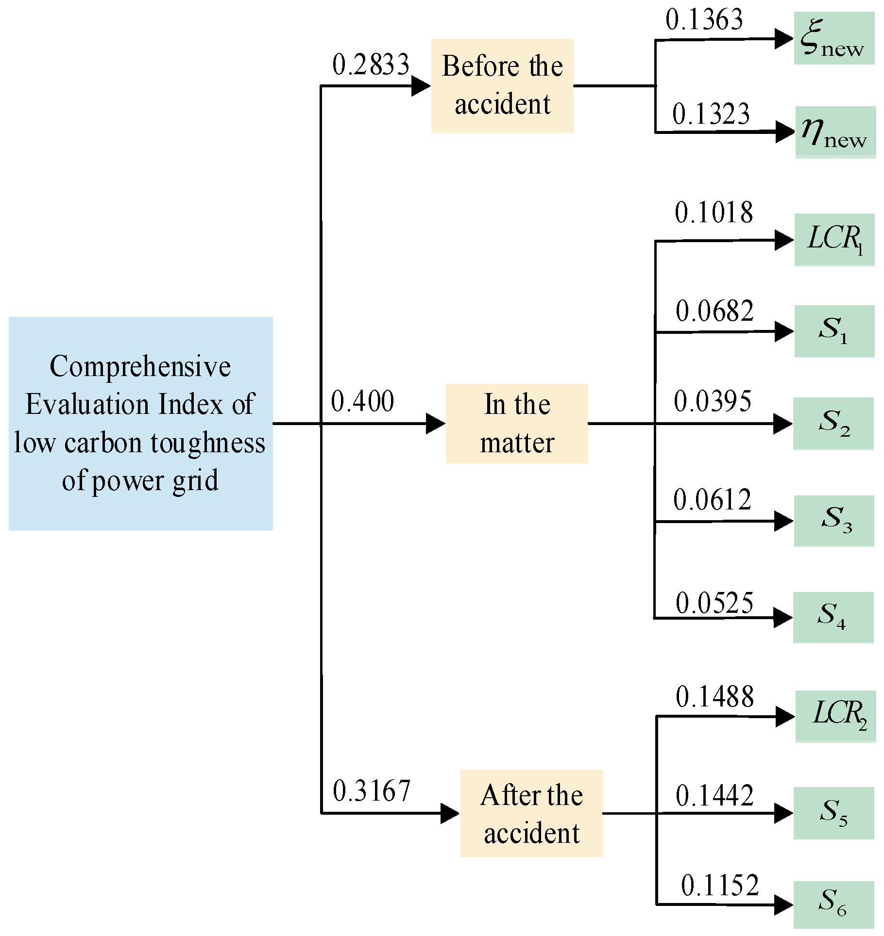
- Considering the impact of the whole process of disaster occurrence on the power grid, we build a comprehensive assessment index system for low-carbon resilience of the power grid; the principal comprehensive weight determination method combined with the fuzzy analytic hierarchy method (FAHP) and anti-entropy weight method (AEWM) is used, and the fuzzy evaluation value obtained is accurately processed with the center of gravity method (COG).
2. LCR
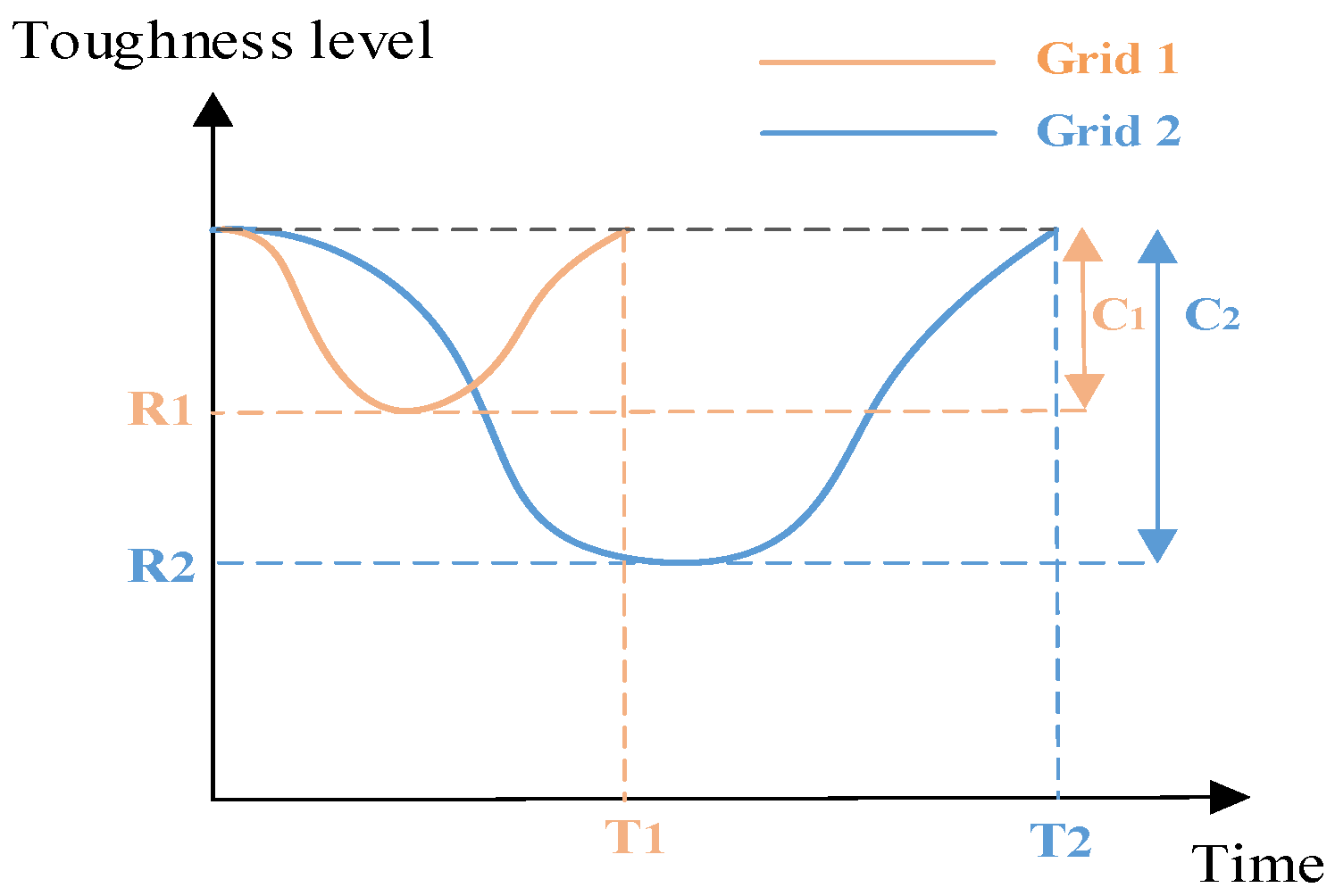
2.1. LCR Concept
2.2. LCR Power Grid
3. Construction of LCR Index System
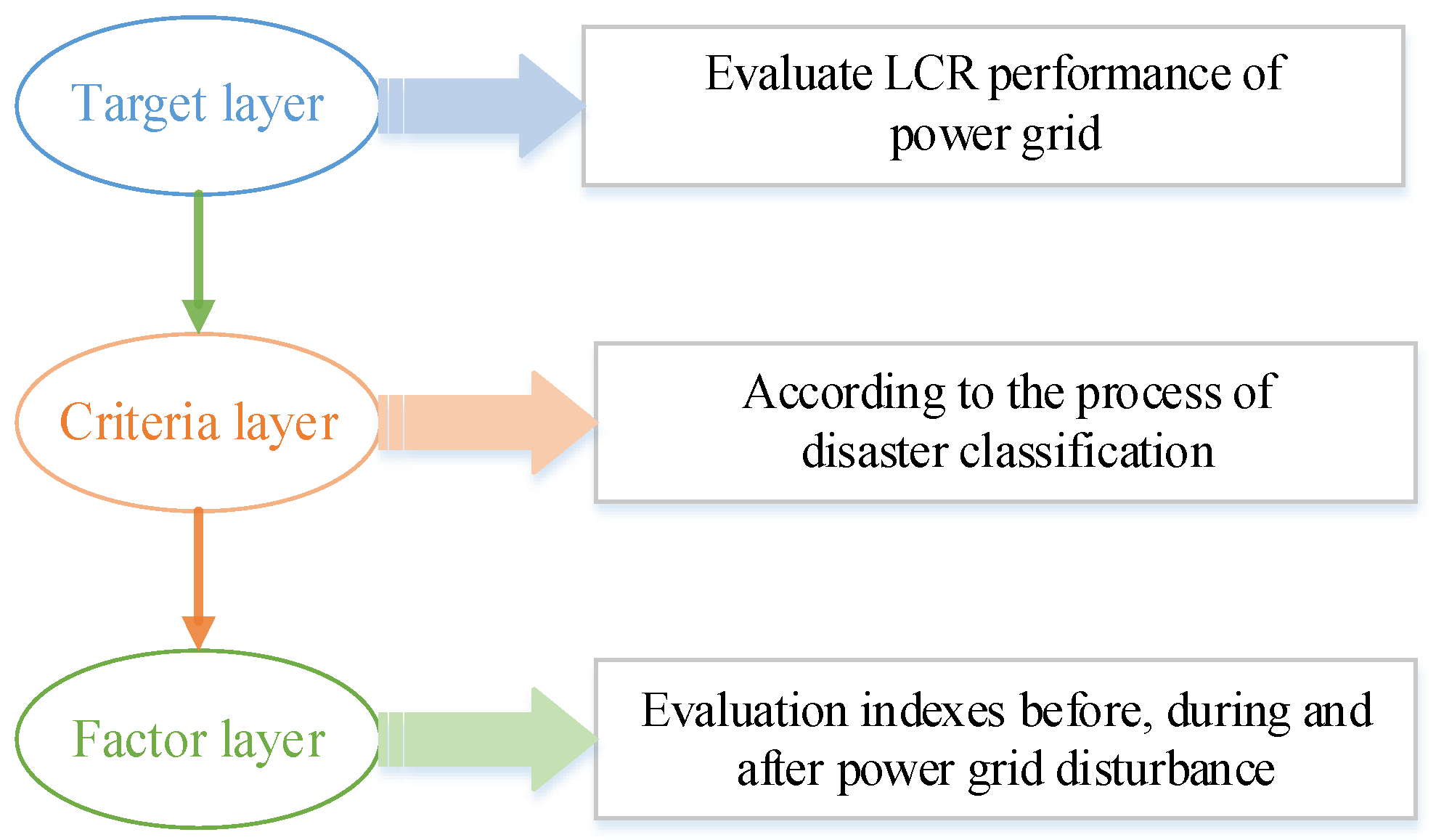
3.1. LCR Key Indicator System
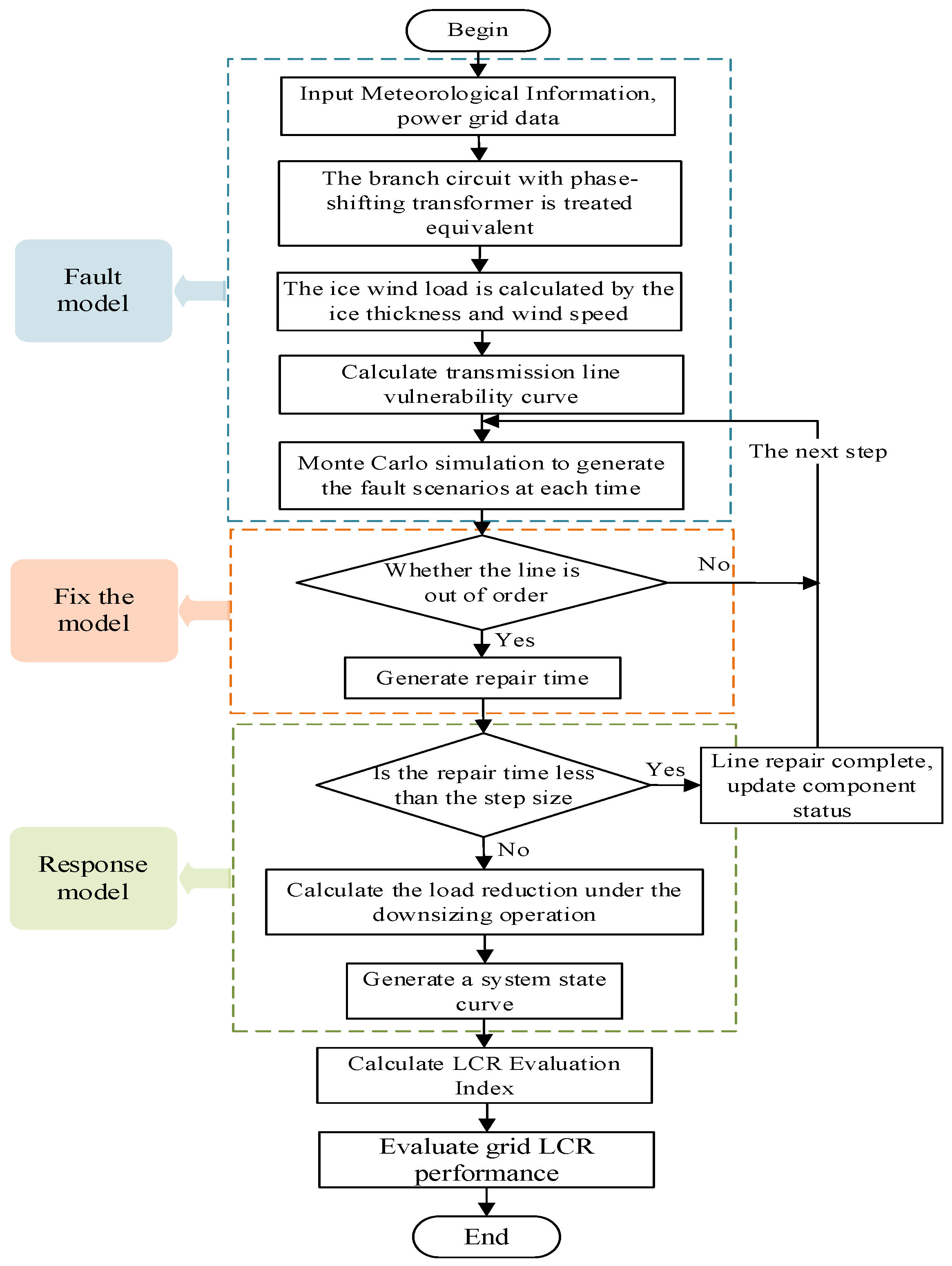
3.2. LCR Grid Assessment Process
3.2.1. Branch Equivalent Model with Phase-Shifting Transformer
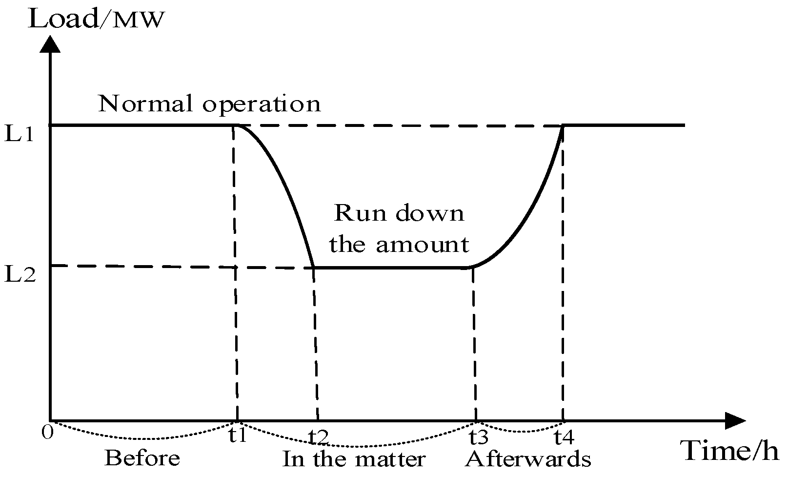
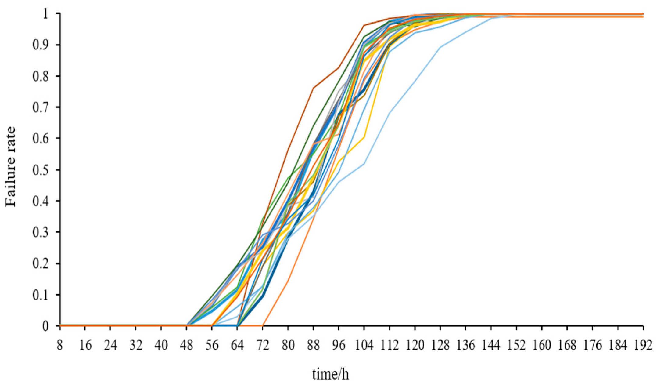
3.2.2. Transmission Line Fault Model
3.2.3. Power System Repair and Response Model
4. LCR Index Evaluation Realization
4.1. FAHP–AEWM-Based Weight Setting
4.1.1. Fuzzy Analytic Hierarchy Process
- Step 1: Establishing the hierarchical model
- Step 2: Constructing the fuzzy complementary judgment matrix
- Step 3: Weight solution
- Step 4: Consistency test
- Step 5: Determining the subjective weight of indicators
4.1.2. Anti-Entropy Weight Method
- Step 1: Standardization of indicators
- Step 2: Determine the anti-entropy value of each index
- Step 3: The objective weight of the index is as follows:
4.2. Comprehensive Evaluation of Indicators Based on FCE–COG
- Step 1: Determine the factor set of the evaluation object
- Step 2: Determine the comment set
- Step 3: Determine the fuzzy judgment matrixwhere is the degree of subordination for . The normal membership function is selected as the membership function of each evaluation index to the comment set [31], which is the standard deviation of the comment set.
- Step 4: Calculate the fuzzy comprehensive evaluation set
- Step 5: Calculate the center of gravity
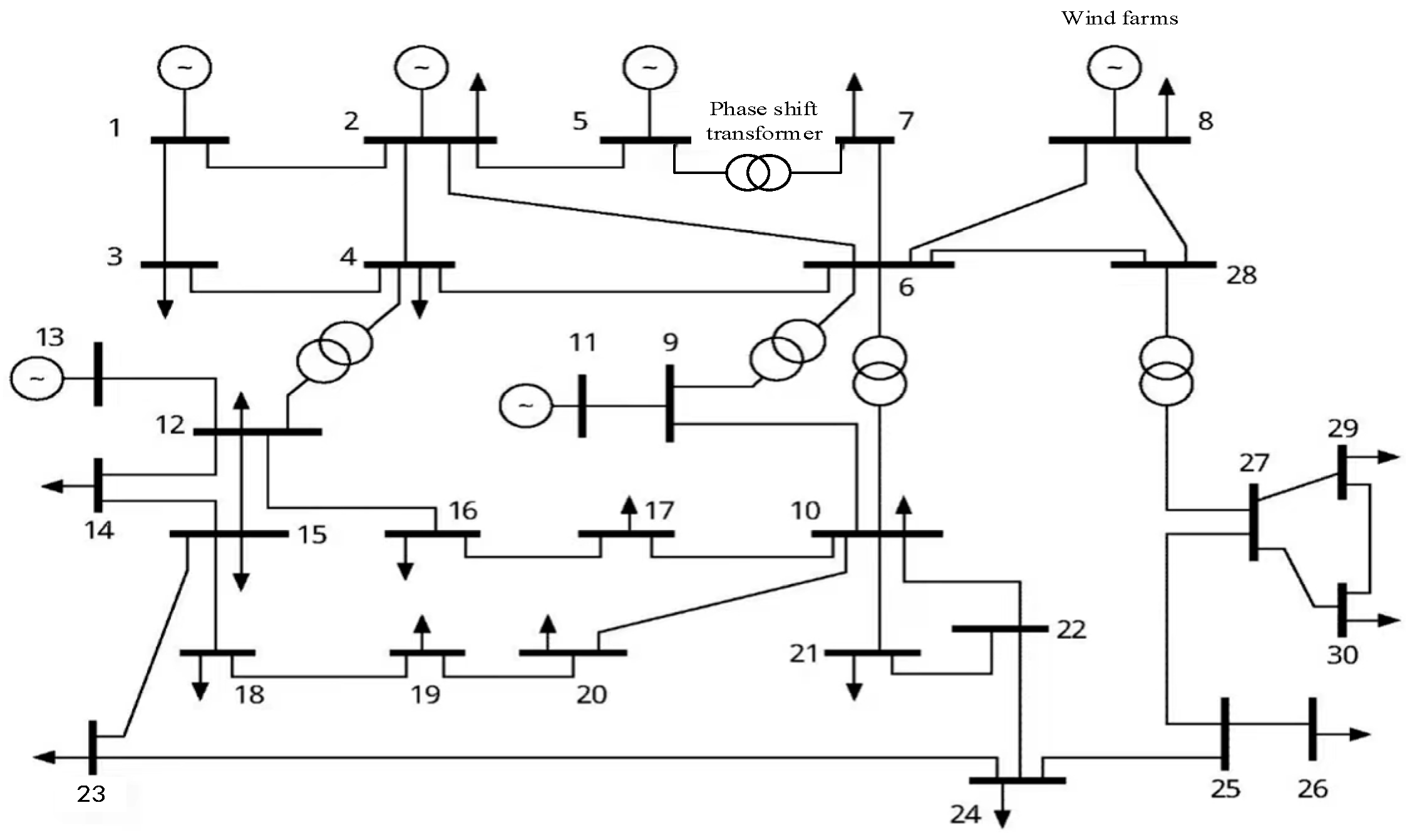
5. Example Analysis
5.1. The Index Value Is Calculated
5.2. Subjective Weight Assignment
5.3. Objective Weight Assignment
5.4. Comprehensive Evaluation
5.5. Results Analysis
6. Conclusions
Author Contributions
Funding
Data Availability Statement
Conflicts of Interest
Nomenclature
| Indices and Sets | |
| e, f | Index for buses |
| m | Index for scenarios |
| Index for the relative importance of each index at the same level | |
| Index for degree of subordination for | |
| Set for loads, generators, lines, nodes | |
| Parameters | |
| NDG | Number of new energy power plants |
| N | Number of buses |
| M | Number of new energy source buses |
| T | Duration of the ice disaster |
| Increase in carbon emissions of the power grid | |
| Time for carbon emissions of the power grid to recover | |
| Carbon emission coefficients of the power plant | |
| New energy emission reduction coefficient | |
| Electricity penetration of new energy sources | |
| New energy generation absorption rate | |
| Thickness of ice cover (mm) | |
| Ice load (N/m) | |
| Wind load (N/m) | |
| Pitch factor | |
| Wind speed (m/s) | |
| The expected value | |
| The standard deviation | |
| The characteristic matrix of the judgment matrix | |
| a | Evaluation index |
| Constants | |
| The amount of load under normal system operating conditions | |
| The amount of load under system derating operation | |
| , | Threshold value |
| Density of ice, 0.9 g/cm3 | |
| Density of water, 1.0 g/cm3 | |
| Wire diameter | |
| Optimistic time for line recovery | |
| Pessimistic time for line recovery | |
| Most likely time for line recovery | |
| The active load of load d | |
| The minimum and maximum output of a generator | |
| Long-term emergency limit of Line Power flow under fault condition | |
| Variables | |
| System operating time: moment of the disaster occurrence | |
| Moment the power grid enters a stable operation at reduced capacity | |
| The moment when the ice disaster dissipates | |
| The moment when the power grid resumes normal operation | |
| Load shedding amount of the system in normal operating conditions | |
| Load shedding amount of the system in a fault state | |
| New energy grid-connected power in fault operating conditions | |
| New energy grid-connected power in normal operating conditions | |
| Power of new energy units i for time period t | |
| Power of load m for time period t | |
| Power of new energy units i or time period t | |
| Load at time period t | |
| , | Additional active power injected into the bus |
| , | Additional reactive power injected into the bus |
| , | Voltage amplitudes of the bus |
| No-load phase-shifting angle of the phase-shifting transformer | |
| Equivalent admittance of the phase-shifting transformer | |
| Bus phase difference of the two sides of the phase-shifting transformer | |
| The precipitation per hour (mm/h) | |
| Wind speed at the location (m/s) | |
| Content of liquid water in the air, | |
| Load d the amount of load cut off in the failure state | |
| Active power output of generator j under fault condition | |
| Power flow of Line l in a fault state | |
| The voltage phase angle of the beginning node d and the end node e of line l under fault condition | |
| The DC resistance of line l | |
References
- Chen, L.; Deng, X.Y.; Chen, H.K.; Shi, J. Power System Resilience Assessment and improvement. Power Syst. Prot. Control. 2022, 50, 11–22. [Google Scholar]
- Ruan, Q.T.; Xie, W.; Xu, Y.; Hua, B.; Song, P.; He, J.H.; Zhang, Q.Q. Concept and key features of flexible power grid. Chin. J. Electr. Eng. 2020, 40, 6773–6784. [Google Scholar]
- Fotopoulou, M.; Rakopoulos, D.; Petridis, S. Decision Support System for Emergencies in Microgrids. Sensors 2022, 22, 9457. [Google Scholar] [CrossRef] [PubMed]
- Wu, Y.K.; Chen, Y.C.; Chang, H.L.; Hong, J.S. The Effect of Decision Analysis on Power System Resilience and Economic Value During a Severe Weather Event. IEEE Trans. Ind. Appl. 2022, 58, 1685–1695. [Google Scholar] [CrossRef]
- Li, Z.K.; Wang, F.S.; Gu, W.Y.; Mi, Y.; Ji, L. Elasticity assessment of smart distribution networks in extreme weather. Power Syst. Autom. 2020, 44, 60–68. [Google Scholar]
- Wang, Y.; Huang, T.; Li, X.; Tang, J.; Wu, Z.; Mo, Y.; Xue, L.; Zhou, Y.; Niu, T.; Sun, S. A Resilience Assessment Framework for Distribution Systems Under Typhoon Disasters. IEEE Access 2021, 9, 155224–155233. [Google Scholar] [CrossRef]
- Chen, Y.; Yang, Y.; Liu, Y.; Lu, Q.; Yang, M.; Zhang, R.; Liu, J. An Optimization Strategy for Power System Partition Recovery Considering Grid Reconfiguration Efficiency and Path Reliability. In Proceedings of the 2023 6th International Conference on Energy, Electrical and Power Engineering (CEEPE), Guangzhou, China, 12–14 May 2023; pp. 1449–1454. [Google Scholar]
- Ruan, Q.T.; Mei, S.W.; Huang, X.D.; Chen, Y. Challenges and prospects for improving the resilience of low-carbon urban power grids. Chin. J. Electr. Eng. 2022, 42, 2819–2830. [Google Scholar]
- Kang, C.Q.; Yao, L.Z. Key scientific problems and theoretical research framework of high-proportion renewable energy power system. Power Syst. Autom. 2017, 41, 1–11. [Google Scholar]
- Milano, F.; Dörfler, F.; Hug, G.; Hill, D.J.; Verbič, G. Foundations and challenges of low-inertia Systems (Invited Paper). In Proceedings of the 2018 Power Systems Computation conference-(PSCC), Dublin, Ireland, 11–15 June 2018. [Google Scholar]
- Shen, T. Application of Phase-Shifting Transformer in Power System; North China Electric Power University: Beijing, China, 2018. [Google Scholar]
- Qu, Z.Y.; Liao, H.X.; Yu, J.L.; Gao, H.; Su, A.L.; Ge, W.C.; Liu, C. Study on phase-shift transformer location problem to eliminate line overload. Grid Technol. 2002, 25, 30–32+44. [Google Scholar]
- Yu, J.L.; Liu, C. Power flow control based on unified characteristics of phase shifters. Chin. J. Electr. Eng. 1994, 14, 1–5+10. [Google Scholar]
- Cui, X.; Zhao, K.; Zhou, Z.; Huang, P. Examining the uncertainty of carbon emission changes: A systematic approach based on peak simulation and Resilience Assessment. Environ. Impact Assess. Rev. 2021, 91, 106667. [Google Scholar] [CrossRef]
- Zhang, J.M.; Wang, Y.K.; Xue, Y.S.; Xue, F.; Chang, K. Natural disaster chain-power system-Bayesian network estimation of carbon emission change. Power Syst. Autom. 2023, 47, 1–11. [Google Scholar]
- Wu, J.; LÜ, L.; Huang, Y.; Li, X.C.; Ji, C.L. Evaluation method and lifting strategy of distribution network elasticity in whole disaster process. J. Power Syst. Their Autom. 2021, 33, 32–42. [Google Scholar]
- Xiao, Z.W.; Wang, G.Q.; Zhu, J.M.; Chen, H.J. Evaluation and construction method of power grid resilience capacity for emergencies. Syst. Eng.-Theory Pract. 2019, 39, 2637–2645. [Google Scholar]
- Jones, K.F. A simple model for freezing rain ice loads. Atmos. Res. 1998, 46, 87–97. [Google Scholar] [CrossRef]
- Zhao, N.Y. Resilience Assessment of Transmission System under Ice Disaster and Strategy of Full-Time Resilience Enhancement; Tianjin University: Tianjin, China, 2020. [Google Scholar]
- Feng, W.M. Grid Operation Risk Assessment and Network Protection Considering Ice Disaster; Harbin Institute of Technology: Harbin, China, 2014. [Google Scholar]
- Huang, W.X.; Wu, J.; Guo, Z.H.; Chen, Y.H.; Liu, Z.C. Power Grid Resilience Assessment and differential planning under typhoon disaster. Power Syst. Autom. 2023, 47, 84–91. [Google Scholar]
- Mota, A.A.; Mota, L.T.M.; Morelato, A. Visualization of Power System Restoration Plans Using CPM/PERT Graphs. IEEE Trans. Power Syst. 2007, 1322–1329. [Google Scholar] [CrossRef]
- Tang, W.H.; Yang, Y.H.; Li, Y.J.; Lu, J.Z.; Wu, Q.H. Research on transmission system elasticity evaluation and lifting measures under extreme meteorological disasters. Chin. J. Electr. Eng. 2020, 40, 2244–2254+2403. [Google Scholar]
- Li, J.Q. Research on Risk Evaluation of Intellectual Property Pledge Financing Based on Fuzzy Analytic Hierarchy Method; University of Electronic Science and Technology of China: Chengdu, China, 2021. [Google Scholar]
- Gong, G.B. Diagnosis of Regional Power Grid Development Based on Fuzzy Analytic Hierarchy Process; China University of Mining and Technology: Beijing, China, 2019. [Google Scholar]
- Liu, Q. Application Research on Risk Management of Small-Scale Power Grid Infrastructure Based on Fuzzy Analytic Hierarchy Process; Tianjin University: Tianjin, China, 2018. [Google Scholar]
- Yang, Y.H.; LÜ, Y.J. Consistency test of fuzzy judgment matrix. Stat. Decis. Mak. 2018, 34, 78–80. [Google Scholar]
- Zhang, H.R.; Han, D.; Liu, Y.J.; Song, Y.Q.; Yan, Z.; Sun, Q.; Zhang, Y.B. Evaluation of smart grid based on anti-entropy weight method. Power Syst. Prot. Control. 2012, 40, 24–29. [Google Scholar]
- LÜ, P.P.; Zhao, J.Q.; Li, D.C.; Zhu, Z.F. Evaluation index system and comprehensive evaluation method. Grid Technol. 2015, 39, 2245–2252. [Google Scholar]
- Zhang, Y. Application Research Based on Fuzzy Analytic Hierarchy-Fuzzy Comprehensive Evaluation Model; Anqing Normal University: Anqing, China, 2022. [Google Scholar]
- Zeng, Y.; Jia, H.P.; Yang, J.; Wang, W.; Zhong, Y.; Han, J.S.; Liu, D.N. Evaluation method of synthetic contribution degree of virtual power plant based on fuzzy analytic hierarchy process-entropy weight method-approximate ideal solution ordering method. Mod. Electr. 2023, 1–8. [Google Scholar] [CrossRef]
- Lin, J.K.; Li, T.F.; Zhao, Z.M.; Zheng, W.H.; Liu, T. Black-start scheme evaluation of power system based on entropy weight fuzzy comprehensive evaluation model. Grid Technol. 2012, 36, 115–120. [Google Scholar]


| Indicator | No Phase Shift Transformer Added | The Phase-Shifting Transformer | Indicator Type |
|---|---|---|---|
| 0.529 | 0.529 | LC | |
| 0.742 | 0.891 | LC | |
| 143.93 MW | 90.991 MW | LCR | |
| 50.2 MW | 42.3 MW | R | |
| 2.258 MW/h | 3.419 MW/h | R | |
| 0.9024 | 0.9613 | R | |
| 0.823 | 0.8792 | R | |
| 56 h | 40 h | LCR | |
| 24 h | 16 h | R | |
| 16.217 MW/h | 18.675 MW/h | R |
| Case | Criteria Layer | Evaluation Matrix |
|---|---|---|
| case 1 | 0.0466, 0.1672, 0.2714, 0.1997, 0.0666 | |
| 0.0412, 0.1673, 0.3136, 0.2717, 0.1089 | ||
| 0.0411, 0.1825, 0.3687, 0.3381, 0.1406 | ||
| case 2 | 0.0666, 0.1997, 0.2714, 0.1672, 0.0466 | |
| 0.1089, 0.2717, 0.3136, 0.1673, 0.0412 | ||
| 0.1406, 0.3381, 0.3687, 0.1825, 0.0411 |
| Case | The Barycenter Vector of the Fuzzy Set in the Criterion Layer | Final Evaluation Indicators and Evaluation Results |
|---|---|---|
| case 1 | 0.4207, 0.4069, 0.4038 | (general) |
| case 2 | 0.5793, 0.5931, 0.5962 | (general) |
Disclaimer/Publisher’s Note: The statements, opinions and data contained in all publications are solely those of the individual author(s) and contributor(s) and not of MDPI and/or the editor(s). MDPI and/or the editor(s) disclaim responsibility for any injury to people or property resulting from any ideas, methods, instructions or products referred to in the content. |
© 2023 by the authors. Licensee MDPI, Basel, Switzerland. This article is an open access article distributed under the terms and conditions of the Creative Commons Attribution (CC BY) license (https://creativecommons.org/licenses/by/4.0/).
Share and Cite
Zhang, J.; Cheng, H.; Yang, P.; Zhang, B.; Zhang, S.; Lu, Z. Comprehensive Evaluation Index System and Application of Low-Carbon Resilience of Power Grid Containing Phase-Shifting Transformer under Ice Disaster. Processes 2023, 11, 2633. https://doi.org/10.3390/pr11092633
Zhang J, Cheng H, Yang P, Zhang B, Zhang S, Lu Z. Comprehensive Evaluation Index System and Application of Low-Carbon Resilience of Power Grid Containing Phase-Shifting Transformer under Ice Disaster. Processes. 2023; 11(9):2633. https://doi.org/10.3390/pr11092633
Chicago/Turabian StyleZhang, Jing, Huilin Cheng, Peng Yang, Bingyan Zhang, Shiqi Zhang, and Zhigang Lu. 2023. "Comprehensive Evaluation Index System and Application of Low-Carbon Resilience of Power Grid Containing Phase-Shifting Transformer under Ice Disaster" Processes 11, no. 9: 2633. https://doi.org/10.3390/pr11092633