Article

Optimal Dispatch of the Source-Grid-Load-Storage under a High Penetration of Photovoltaic Access to the Distribution Network

1
School of Electrical Engineering, Tibet Agriculture and Animal Husbandry University, Linzhi 860000, China
2
Research Center of Civil, Hydraulic and Power Engineering of Tibet, Linzhi 860000, China
3
Linzhi Power Supply Company, State Grid, Linzhi 860000, China
4
College of Water Conservancy and Civil Engineering, Tibet Agriculture and Animal Husbandry University, Linzhi 860000, China
*
Author to whom correspondence should be addressed.
Processes 2023, 11(10), 2824; https://doi.org/10.3390/pr11102824
Submission received: 26 August 2023 / Revised: 23 September 2023 / Accepted: 23 September 2023 / Published: 25 September 2023
(This article belongs to the Special Issue Advances in Electrical Systems and Power Networks)

Abstract

:
In the context of carbon peaking and carbon neutralization, distributed photovoltaics is a relatively mature new energy power generation technology that is being widely promoted. However, the randomness and volatility of distributed generation bring severe challenges to the distribution network’s operation. Based on this, taking the typical scenario of a high proportion of distributed photovoltaic grid connections against the background of a whole-county photovoltaic system as the research object, this paper constructs a source-grid-load-storage coordination optimal scheduling model in distribution networks, considering the spatial distribution of power flow, tie-line power fluctuation, grid loss, and voltage amplitude from the perspective of optimal day-to-day scheduling. Next, the Lehmer weighted and improved multi-mutation cooperation strategy differential evolution (LW-IMCSDE) algorithm is introduced to enhance the differential evolution algorithm based on the weighted Lehmer average, improved multi-mutation cooperation, and population update strategies. The feasibility and effectiveness of the algorithm are investigated by using a test function to verify its effectiveness. Finally, the feasibility and effectiveness of the proposed strategy are verified in two typical power scenarios: summer and winter.

1. Introduction

In the context of carbon peaking and carbon neutralization, the new energy represented by distributed photovoltaics (PVs) shows a high proportion of access [1]. However, the randomness and volatility of distributed PV output bring severe challenges to the distribution network’s safe and stable operation when there is a high proportion of access [2]. Therefore, the aspects of large-scale grid connection of distributed PVs and the optimal scheduling strategy of source-grid-load-storage in distribution networks [3] have become important aspects in the research field of new power systems [4].
Given the randomness and volatility of new energy output, a centralized or decentralized energy optimization control strategy can be adopted [5]. Some scholars have established a multi-timescale energy optimization model and proposed a rolling optimal scheduling strategy [6,7,8] that considers the uncertain response model of time-sharing electricity prices and the time response characteristics of an interruptible load. In ref. [9], the interruptible load is taken as the reserve capacity of the system, and the user-side interactive dispatching model is established to deal with the reverse peak regulation and volatility of wind power. Refs. [10,11] put forward the integrated operation mode of source-grid-load-storage energy control and economic operation at the park and system levels, which verifies the economy and sustainability of source-grid-load-storage coordination and optimization of the operation mode. An affine, adjustable, and robust reactive power optimization algorithm is proposed in [12]. By adjusting the grid’s reactive power flow, the system loss and node voltage are optimized. Ref. [13] takes the microgrid group as the research object, focuses on the energy management and power coordination control strategy in the off-grid mode, and realizes the stable operation of the system. However, the current power dispatching optimization strategies mostly study and analyze the equivalence of source-grid-load-storage concentration in the power system, and fail to consider the power flow operation state on a spatial scale [14].
Traditionally, power systems consist of three parts: generation source, transmission grid, and load demand. In the future, energy storage will also become an indispensable part of power systems, since more flexibility is required to render the optimal operation of systems with high penetration of variable energy resources. There have been many studies focused on the establishment of grid dispatching models. Minimizing grid loss [15] and improving voltage quality [16] are often regarded as the optimization objective, and most existing studies have focused on active or reactive power dispatching [17,18]. Therefore, the coupling effect of active and reactive power on grid dispatching is typically not fully considered.
Relevant research has shown that a combined active and reactive optimization strategy is more effective than a single optimization strategy [19], but with a high percentage of distributed PV connected to the grid, the various links in the power system have a wide variety of control variables, higher dimensionality, and more complex calculations, making it difficult to adapt to optimization needs with the help of traditional artificial intelligence algorithms. Ref. [20] used an improved genetic algorithm to optimize a distribution grid containing wind turbines. Ref. [21] improved the differential evolution (DE) algorithm with the help of a penalty function and applied it to the optimization problem of grid-connected photovoltaic and adjustable resources in the power system. Ref. [22] improved the DE algorithm with the help of the Artificial Bee Colony algorithm and applied it to dynamic economic dispatching. Ref. [23] improved the initialization strategy of the DE algorithm in the optimal reactive power scheduling problem and updated the scaling factor and crossover probability using an adaptive adjustment strategy. At present, although artificial intelligence algorithms are widely used in active/reactive power system scheduling optimization [24,25], the proportion of grid-connected renewable energy units such as wind turbines (WTs) and PVs in the above studies is limited. Therefore, in the face of multi-objective optimization problems with a high proportion of distributed PVs connected to the grid, all their improvement strategies have disadvantages, such as the high probability of falling into a local optimum, low convergence accuracy, and difficulty in best-fitness optimization.
Thus, this paper takes the typical scene of a high proportion of distributed PV grid connections in the context of a whole-county PV as the research object, and from the point of view of day-ahead optimal dispatching, a load-storage coordinated optimal dispatching model of the distribution network considering tie-line power fluctuation, grid loss and voltage amplitude is constructed, which takes into account the spatial distribution of power flow. Next, the Lehmer weighted and improved multi-mutation cooperation strategy differential evolution (LW-IMCSDE) algorithm is introduced to improve differential evolution with forward-inverse initialization, weighted Lehmer average, multi-mutation cooperation strategy, and an updated population strategy algorithm to improve global merit-seeking ability and convergence speed of the algorithm in the face of high-dimensional variables. Finally, the performance of the algorithm is examined using three commonly used test functions, and we analyze and verify the effectiveness of the model construction and the proposed strategy through the IEEE’s classical model.

2. Multi-Objective Optimal Scheduling Model of Source-Grid-Load-Storage

2.1. Optimization Goal

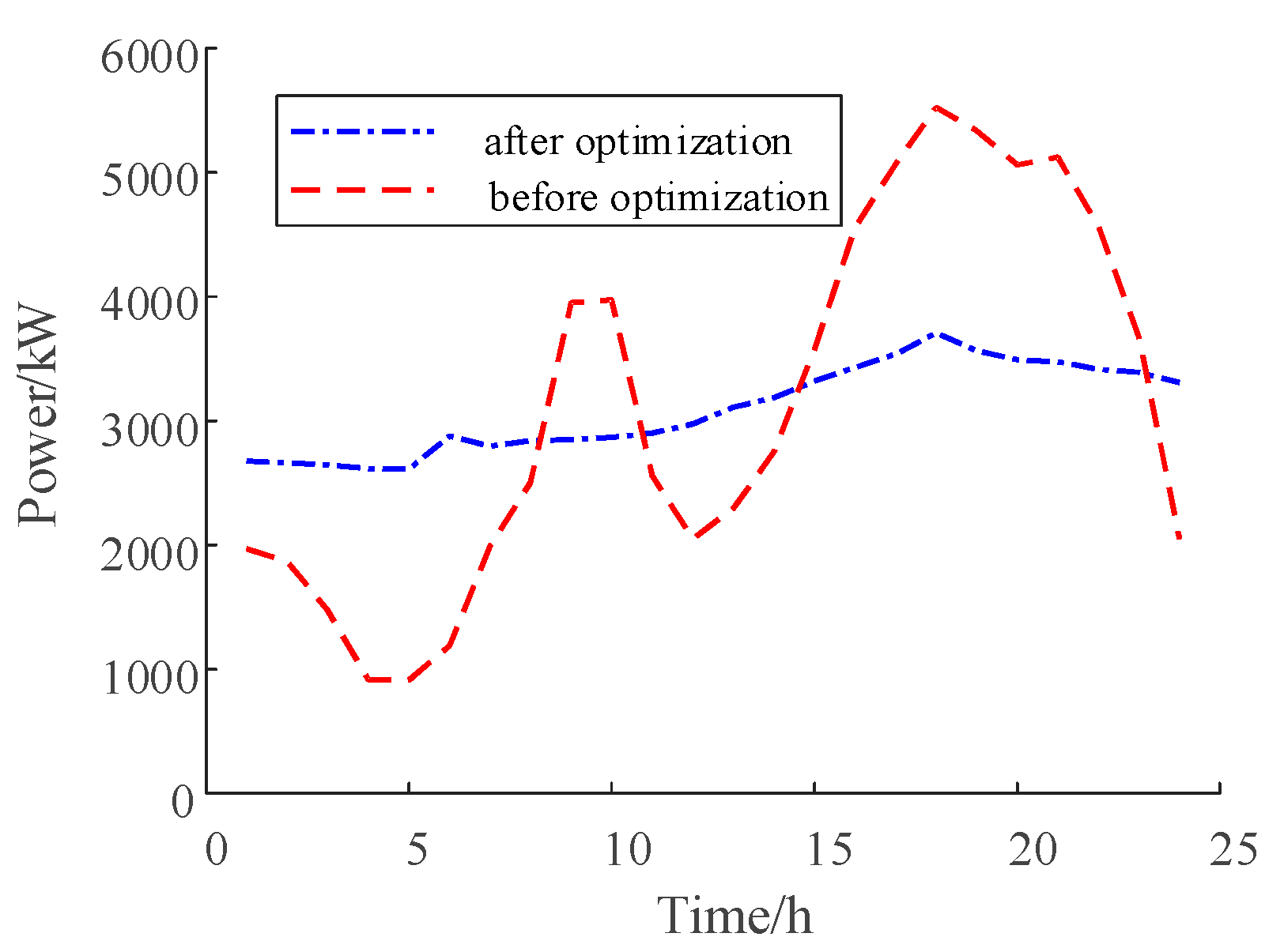
2.1.1. Fluctuating Tie-Line Power between the Distribution Network and Power Grid
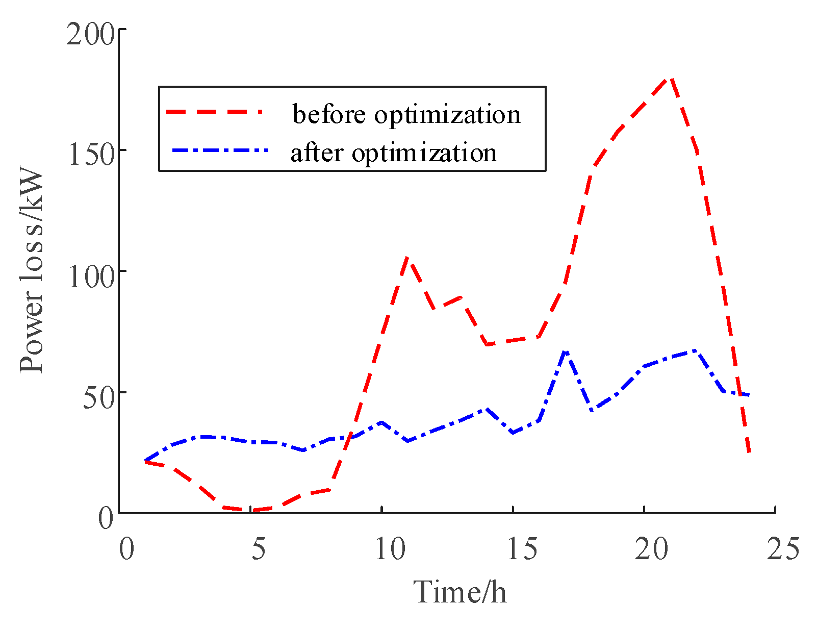
To some extent, the fluctuation of tie-line power can reflect the influence of the distribution network on the large power grid. There are two main evaluation indexes to reflect changes in tie-line power, namely the change rate of tie-line power and the fluctuation rate of tie-line power [26,27]. The change rate of tie-line power is defined as:
D grid = P grid , max P grid , min Δ t
where D grid is the power change rate of the tie line. P grid , max and P grid , min are the maximum and minimum values of tie-line power in Δ t time interval, respectively. The volatility of tie-line power is expressed by the standard deviation of tie-line power, as shown in Formula (2).
δ grid = 1 T 1 t = 1 T ( P grid , t P grid , a v ) 2
In this formula, δ grid is the tie-line volatility. P grid , av is the average power of the tie-line, and P grid , t is the power of the tie line at time point t , t T .

2.1.2. Grid Loss

Grid loss is an important economic index of grid power flow optimization. The reasonable setting of the states of various distributed devices in the system and the active output of a multi-energy complementary distribution network system can improve the power flow distribution of the system and effectively control the grid loss of the system. The mathematical expression is as follows:
P loss = n = 1 N V n m M V m ( G n m cos δ n m + B n m sin δ n m )
In this formula, P loss represents the grid loss of the system. V n and V m are the voltage amplitudes of nodes n and m , respectively. G n m , B n m , and δ n m represent the conductance, admittance, and phase angle difference between nodes n and m . N is the total number of nodes and M represents the set of nodes connected to node m .

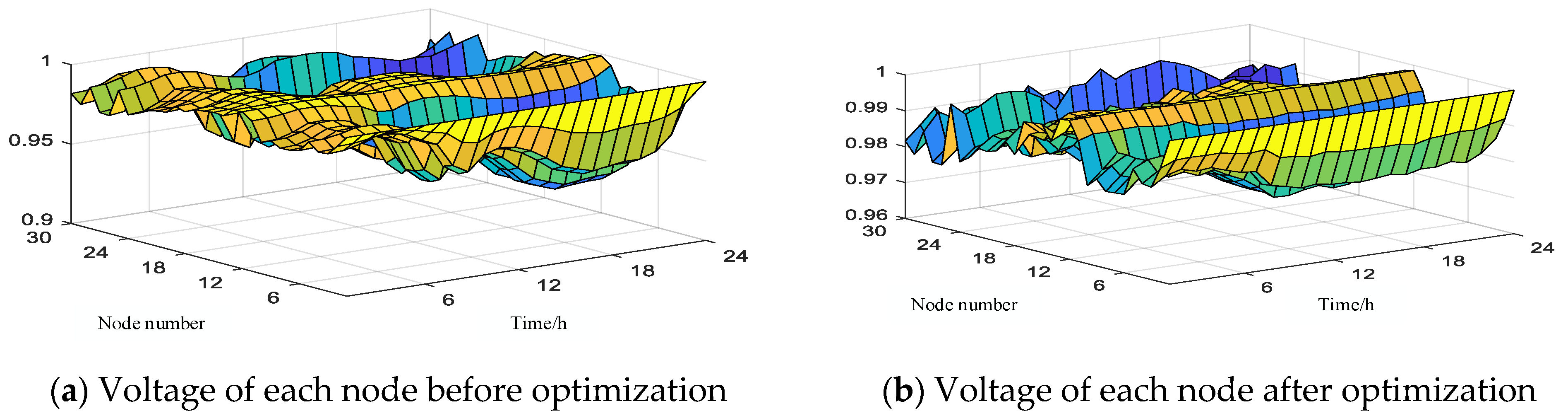
2.1.3. Node Voltage Deviation

The voltage amplitude of the node is one of the important indexes of power quality. This is especially true after a large-scale grid connection of distributed PVs when the power flow direction of the distribution network becomes more complex and diverse, which increases the risk of the voltage amplitude of the line node exceeding the limit. By adjusting the reactive power of a PV grid-connected inverter, the system node voltage can be effectively optimized. The mathematical expression is:
U grid = 1 N 1 b = 1 N ( U n U s ) 2
In this formula, U grid is the node voltage deviation rate. U n is the n node voltage amplitude. U s is the standard voltage amplitude.

2.2. Constraint Condition

2.2.1. Electric Power Balance Constraint
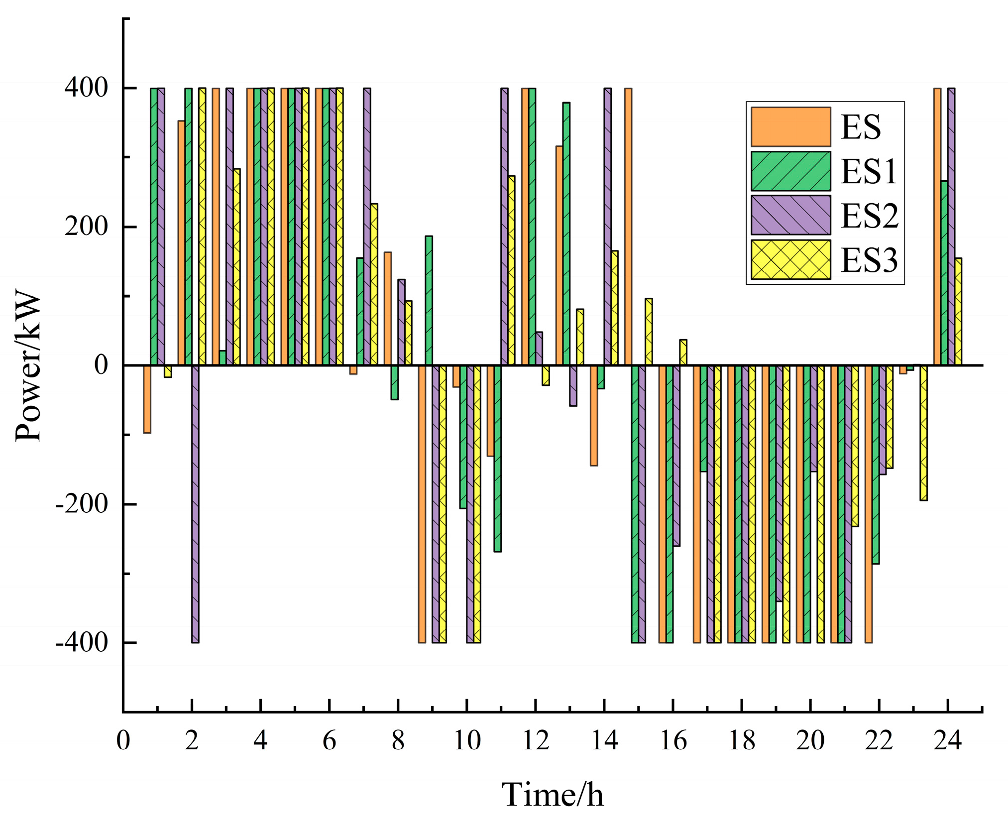
P grid , t + x = 1 N pv P pv , x , t = l = 1 N le P le , l , t + z = 1 N ke P ke , z , t + y = 1 N se P se , y , t
where P pv , x , t is the x th PV t period active power. P le , l , t is the l th load t period power. P ke , z , t is the z th controllable load t period power. P se , y , t is the y th t period charge and discharge power of the energy storage (ES) device.

2.2.2. ES Model

The ES constraints can be expressed as follows:
(1)
Power constraints of ES equipment:
K se , b P se , min P se , y , t K se , b P se , max
where K se , b is the state of the distributed ES unit ( b = 1 means operation, b = 0 means outage). P se , min and P se , max are the lower and upper limits of the power of the distributed ES unit.
(2)
Capacity constraints of ES:
S se , min S se , y , t S se , max
where S se , min and S se , max are the upper and lower limits of the ES capacity of each distributed ES device unit, and S se , y , t is the ES capacity of the t period of the i th distributed ES device unit.
(3)
Charge and discharge balance constraints of ES equipment:
{ S se , y , t = S se , y + P se , y , t t = 1 T P se , y , t = 0
where P se , y , t is the charge and discharge power of the y th ES device in t period. S se , y is the initial ES capacity.

2.2.3. Controllable Load Model

The controllable load constraints can be expressed as follows:
(1)
Controllable load power constraints:
K le , a P le , z , min P le , z , t K le , a P le , z , max
where K le , a is the state of distributed controllable load ( a = 1 means operation, a = 0 means outage). P le , z , max and P le , z , min are the upper and lower limits of z th distributed controllable load power.
(2)
Controllable load electricity constraint:
{ P ke , z , t = P le , z , t S le , z , t 0 S le , z , t S le , z , max
where S le , z , max is the upper limit of energy consumption of the distributed controllable load, and S le , z , t is the power consumption of the z th controllable load t period.

2.2.4. Line Power and Grid State Constraints

Assuming that the grid meets the requirements of open-loop operation and the line power does not cross the line, by adjusting the switch displacement information in the distribution network, the grid state constraints can be expressed as follows:
S c , min S c , t S c , max
where S c , max and S c , min are the upper and lower limits of the apparent power of the m th line, and S c , t is the apparent power of the t period of the c th line.
N c ( A s ) = 0       ( s = 1 , 2 , ... , n s )
where A s is the s th grid topology state, N c ( A s ) is the number of electrical loops in the s th grid topology state, and n s is the total number of grid topology states.

2.2.5. PV Inverter Constraints

Considering the constraints of PV inverter power and operating conditions, the reactive power of the PV grid-connected inverter is fully used, and the PV inverter constraints can be expressed as follows:
{ 0 P pv , x , t P pv , x , max P pv , x , t 2 + Q pv , x , t 2 S pv , x , t 2 tan θ x , t P pv , x , t Q pv , x , t P pv , x , t tan θ x , t
where P pv , x , max is the x th PV t period output power, S pv , x , t is the x th PV t period apparent power, Q pv , x , t is the x th PV t period reactive power, and θ x , t is the x th PV t period inverter power factor angle.

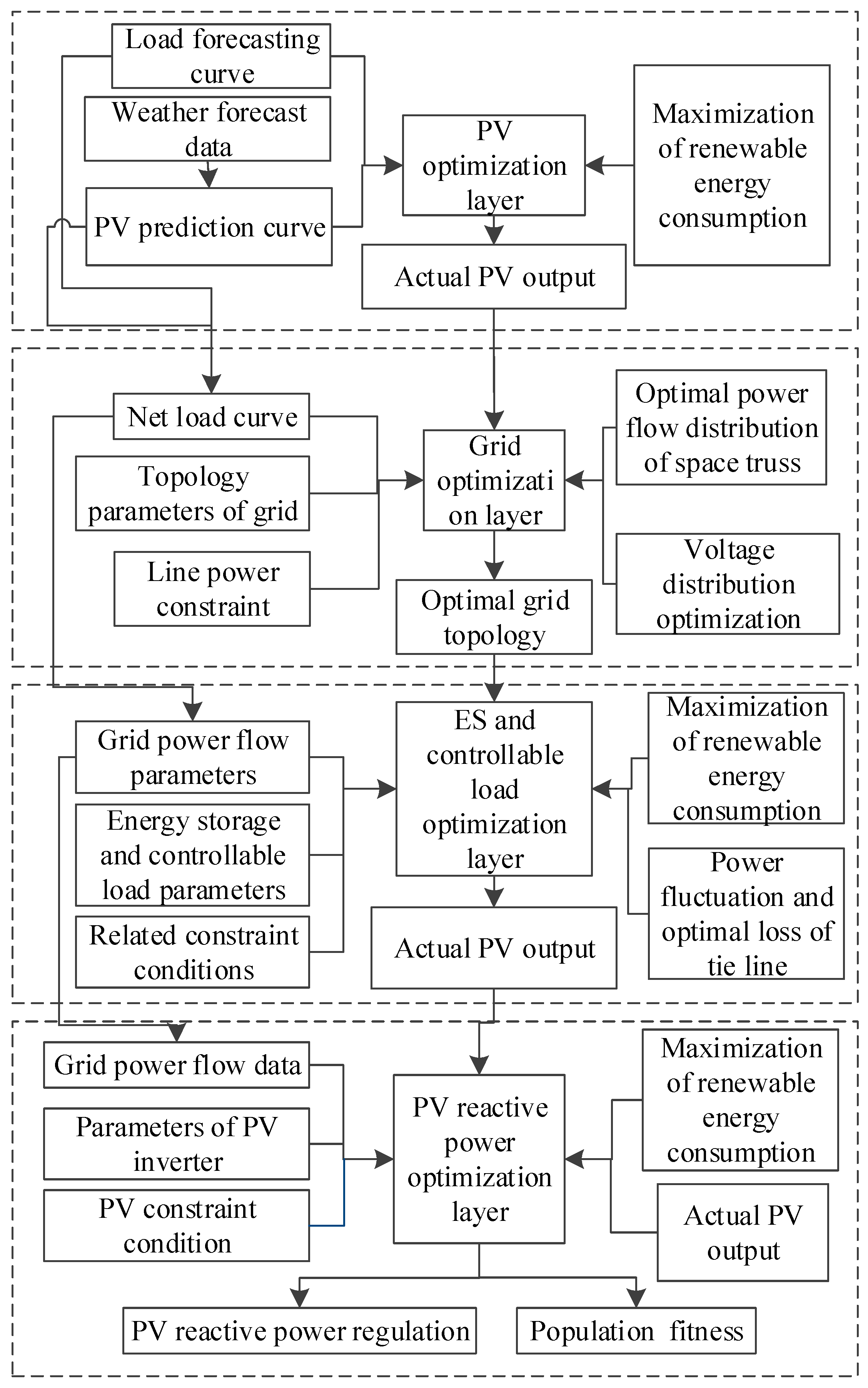
3. Hierarchical Solution Strategy of the Model

Hierarchical Optimization Framework

In this paper, the hierarchical solution framework of the model is divided into four levels. Through the coordination and optimization of all levels, the multi-objective optimization regulation of the load and storage of the distribution network under the background of high-proportion PV access is realized. The concrete framework is shown in Figure 1.
PV optimization layer: To maximize the consumption of PV output, the PV output curve is predicted by meteorological data, and the net load curve is calculated by combining the load curve and the PV output prediction curve. The results are then transmitted to the next layer.
Grid optimization layer: Assuming that the grid meets the requirements of open-loop operation and the line power does not cross the line, by adjusting the switch displacement information in the distribution network, the topology structure of the grid power flow and node voltage distribution are optimized and the power flow distribution of the grid is transferred to the next layer.
ES and controllable load optimization layer: Considering the power and electric quantity constraints of ES and controllable loads, after optimizing charging, discharging, and electric power consumption and reducing the power fluctuation and grid loss of tie lines, the optimized grid power flow distribution is transferred to the next layer.
PV reactive power optimization layer: Considering the constraints of PV inverter power and operating conditions, the reactive power of the PV grid-connected inverter is fully used, the node voltage of the grid is adjusted, and the power quality is improved.
Finally, after multi-level optimization, the fitness of the optimization scheme is assessed through normalization.

4. LW-IMCSDE Algorithm

The LW-IMCSDE algorithm is introduced to address the problems of complex models, the high dimensionality of variables, and difficulties in optimization for the high-proportion distributed PV grid connection optimization problem, as shown below.

4.1. Algorithm Initialization

p o p i , j T = ( p o p i , 1 T , p o p i , 2 T , ... p o p I , D T )
S p o p i , j 0 = p o p j , min + r a n d ( p o p j , max p o p j , min ) P p o p k , j 0 = r a n d ( p o p j , max p o p j , min ) p o p i , j
{ p o p i , j 0 = S p o p i , j 0 ,   i f   f ( S p o p i , j 0 ) < f ( P p o p i , j 0 ) p o p i , j 0 = P p o p i , j 0 ,   otherwise
where S p o p i , j 0 is the forward initialization, P p o p i , j 0 is the reverse initialization, T in Equation (16) is the number of evolutionary generations, i I is the number of populations, j D is the dimensionality of the variables, f ( ) is the fitness value, and p o p j , max and p o p j , min are the upper and lower limits of the population boundaries, respectively. The forward and reverse initialization further enhance the population diversity compared to the original initialization strategy.

4.2. Lehmer Weighted Correction Strategy

The crossover probability C R of the DE algorithm mainly reflects the magnitude of the amount of information exchanged between children and parents and intermediate variants in the process of crossover. The scaling factor F mainly affects the global merit-seeking ability of the algorithm. In this study, the Lehmer average corrections C R and F are introduced, and the initial values of C R and F are taken as 0.5. The correction strategy is as follows:
{ F n = randn ( F , 0.1 ) C R c = randc ( C R , 0.1 )
{ F n = { 1   if   F n > 1 F n   else   if   0.5 F n 1 0.5   otherwise   F n < 0.5 C R c = { 1   if   C R c > 1   C R c   else   if   0.5 C R c 1 0   otherwise   C R c < 0.5
{ F i n F n C R i c C R c
where randn is the normal distribution and randc is the Cauchy distribution. The Cauchy distribution has maximum distribution characteristics, greatly increasing the randomness of the C R c and providing sufficient samples for the C R , while the F requires a lower sufficiency of selected samples than the C R , which is why the normal distribution is chosen. The C R c and F n values obtained from Equations (17) and (18) are revalued according to different situations to ensure the feasibility of their results.
M F = i = 1 I ω F ( i ) ( F n ) 2 / i = 1 I ω F ( i ) F n
M C R = i = 1 I ω CR ( i ) ( C R c ) 2 / i = 1 I ω C R ( i ) C R c
where M F is the weighted Lehmer average of F and M C R is the weighted Lehmer average of C R . The weights of the weighted Lehmer average strategy are updated based on the adaptation improvement values:
ω C R ( i ) = ω F ( i ) Δ f / i = 1 I Δ f
Δ f = | f c f ( i ) |
where f c is the global optimal fitness reference value, and f ( i ) is the previous generation’s optimal fitness value for the fast correction of weight values. ω C R ( i ) is the corrected weight value of C R , ω F ( i ) is the corrected weight value of F , Δ f is the fitness improvement value, and I is the number of populations.
A F = { ( 1 c ) F i n + c × M F , F i n ( 1 c ) F i n + c × rand ,   otherwise
A C R = { ( 1 c ) C R i c + c × M C R , C R i c ( 1 c ) C R i c + c × rand ,   otherwise
where c is a constant of (0~1), rand is a random number of (0~1), A F is the weighted Lehmer average correction value of F , and A C R is the weighted Lehmer average correction value of C R . The weighted Lehmer average value is added to update A F and A C R to avoid the premature convergence of the strategy, thus preventing it from falling into a local optimum. The weighted Lehmer average correction values A F and A C R replace F and C R in Equation (18) after each iteration, and A F and A C R are continuously corrected by the optimal fitness reference value according to different stages.

4.3. Multi-Mutation Cooperation Strategy

V 1 = { i f   rand > A C R p o p + A F ( G b e s t G b a d ) otherwise G b e s t + A F ( p o p r 1 p o p r 2 )
V 2 = { i f   rand > A C R p o p + A F ( P b e s t G b a d ) + A F ( p o p r 2 G b e s t ) + δ ( x p o p ) otherwise G b e s t + A F ( P p o p S p o p ) + A F ( p o p r 3 - p o p r 4 ) + δ ( x p o p )
V 3 = { i f   rand > A C R N ( p o p + G b e s t 2 , p o p G b e s t ) ,   otherwise p o p r 1 + A F ( G b e s t p o p r 2 ) + A F ( p o p r 2 p o p r 3 ) + δ ( x p o p )
x = i = 1 I G b e s t . i p o p
where N ( · ) is the Gaussian distribution, p o p r 1 , p o p r 2 , p o p r 3 , and p o p r 4 are the four randomly selected individuals in the population, G b e s t is the global best individual in the iterative process, G b a d is the global worst individual in the iterative process, and δ is the weight of influence of the central mean, which plays an important role in the evolutionary process, and together with the value of x represents the degree of learning from the best individual. The value of δ is set to 0.04, and P b e s t is the agent randomly selected from the current optimal individual.
V 1 , V 2 , and V 3 are three parallel mutation strategies, and the optimal mutation strategy is selected by comparing their corresponding fitness values. For high-dimensional variables, the parallel approach of multi-mutation collaborative strategies can greatly improve the optimization-seeking ability.
The global optimality-seeking capability is improved in the mutation strategy V 2 . P b e s t in V 2 uses the global optimum to guide P b e s t to help these individuals jump out of the local optimum when they fall into it. This guidance mechanism can accelerate the convergence of the algorithm. In addition, a strategy of simultaneous crossover and variation is adopted to further enhance the convergence speed of the algorithm.

4.4. Fitness Selection Strategy

{ f ( V T ) = min (   f ( V 1 ) , f ( V 2 ) , f ( V 3 ) ) V = V T
where V is the optimal individual, f ( V T ) is the optimal fitness value of the T th generation, and f ( V 1 ) is the fitness value of the mutation strategy V 1 .
In this paper, the population is updated by replacing the worst individual in the population with p o p n and p o p n is determined by G b e s t , P b e s t , and other coefficients as follows:
P w = { A C R ,   i f   c < A C R 1 A C R ,   otherwise
P s = { 0 ,   i f   f ( V T ) < G b e s t 1 ,   otherwise
P u = [ G b e s t ( n 1 1 ) ( n 2 2 ) + G b e s t P b e s t ( n 3 1 ) ( n 2 2 ) + 1 ( n 4 1 ) ( n 4 2 ) ( n 4 2 ) ] / 3
p o p n = P v P s P u
where P w is the weight of the updated population, P s determines whether to update the population, P u indicates that the updated population is associated with G b e s t and P b e s t , and n 1 + n 2 + n 3 + n 4 = I .

5. Example Analysis

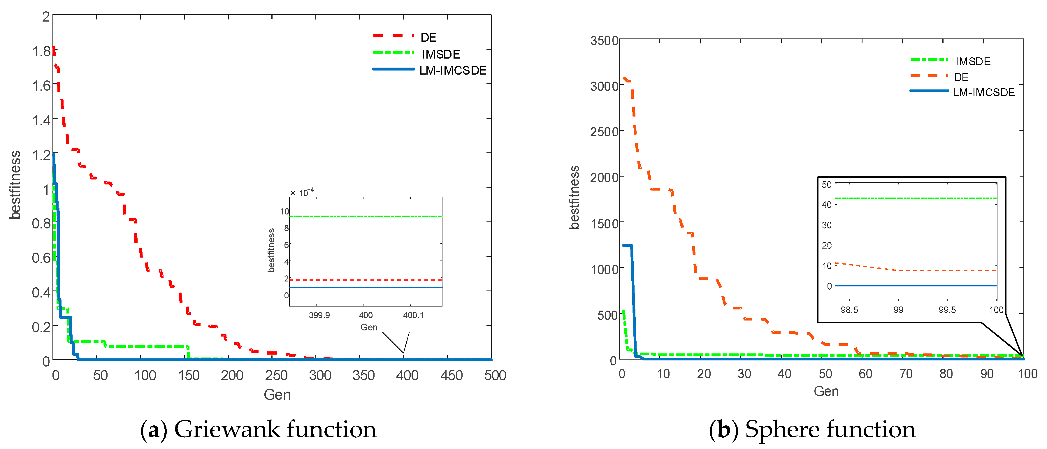
5.1. Algorithm Performance Analysis

To verify the performance of the LW-IMCSDE algorithm, two commonly used test functions are used, as shown in Table 1. The Griewank function is a multi-peak function with the interval [−600, 600]; the sphere function has only the global optimum and an interval of [−600, 600]. The number of individual dimensions of the algorithm is set to 20, and the population size is 100.
Figure 2a,b show the performance comparison with the Griewank, Rastrigin, and sphere functions as the test functions. The IMSDE algorithm is an improved multivariate policy DE algorithm that considers Equations (28)–(31) without considering the weighted Lehmer average improvement.
By looking at the comparison in Figure 2a, we can see that the IMSDE algorithm and the LW-IMCSDE algorithm have significantly better optimizing speeds than the DE algorithm, but the IMCSDE algorithm has a lower adaptation value than the DE algorithm in the test function and it is easier for it to fall into the local optimum, whereas the LW-IMCSDE algorithm not only has a fast optimizing speed but can also jump out of the local optimum. As can be seen from Figure 2b, the LW-IMCSDE algorithm has an optimal fitness value of 0, which reaches the optimal value of the function, i.e., the global optimization-seeking ability is better.

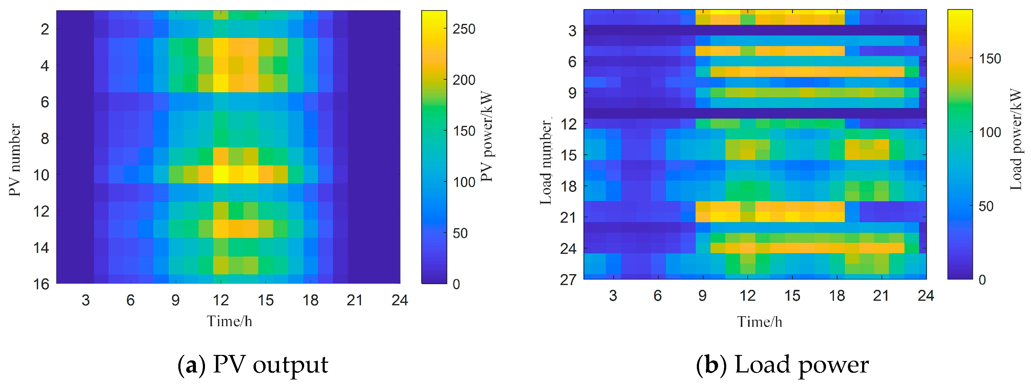
5.2. Calculation of the Basic Situation

In this study, the parameters of IEEE’s typical distribution network model are selected. Under the background of whole-county PV, 16 PV grid points, 4 ES access points, and 2 (11 and 30 points) controllable load access points are set up. The six dotted lines in Figure 3a represent switchable lines, which are used to optimize the grid topology. The optimal grid topology in summer/winter is the same, as shown in Figure 3b.
In this study, by combining meteorological parameters such as light and temperature in a certain place over the past three years, the output scenarios of 16 PV nodes on typical summer and winter days are simulated. In terms of load power, it is divided into three categories: industrial load, commercial load, and residential load. According to the historical load data of a certain place, the paper sets the output scenarios for 27 load nodes on typical days in summer and winter, where Figure 4a shows the PV output power on a typical day in summer and Figure 4b shows the typical daily load in summer. Figure 5a shows the PV output power on a typical day in winter, and Figure 5b shows the typical daily load in winter.

5.3. Simulation Calculation Results

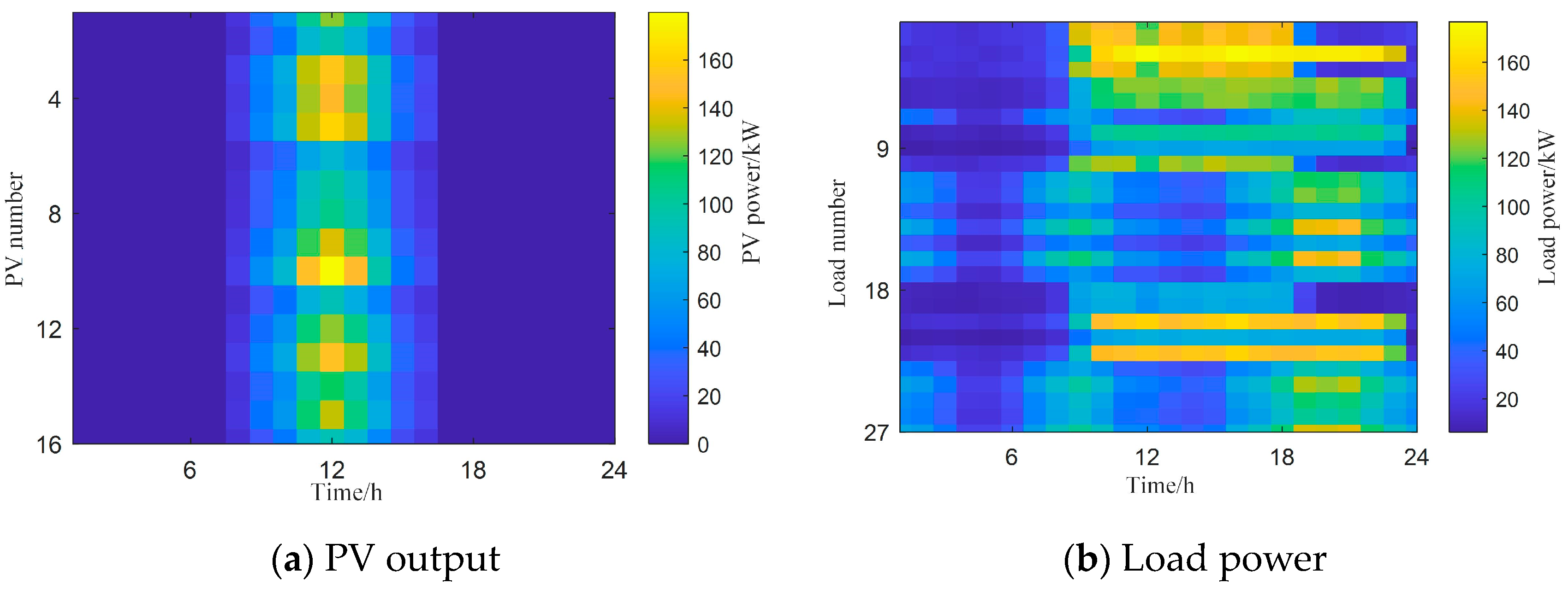
5.3.1. Simulation Calculation of a Typical Day in Summer

The controllable load power and the reactive power of the PV inverter are no longer shown. The ES charging and discharging powers are shown in Figure 6, a comparison of the results before and after node voltage optimization is shown in Figure 7, the power of the tie line before and after optimization is shown in Figure 8, and the grid loss before and after optimization is shown in Figure 9.
Combined with Figure 6, Figure 7, Figure 8 and Figure 9, the grid losses are significantly elevated after 9:00, and at the same time, the power demand on the grid rises. So, to reduce grid losses and interactive power fluctuations, the ES is charged from 1:00 to 9:00. The contact line interactive power is boosted to provide active power dispatch capacity for high grid losses after 9:00, while the PV inverter provides a stable voltage when grid losses are elevated. Then, the reactive power output is boosted.
Finally, the total grid loss was reduced from 1693.43 kW before optimization to 964.82 kW after optimization, with a loss reduction rate of 43.03%. The variance value of the interactive power with the superior grid was reduced from 1.38 before optimization to 0.37 after optimization, and the volatility of the interactive power was significantly reduced. The lower limit of the voltage scale value increased from 0.93 pu before optimization to 0.97 pu after optimization.

5.3.2. Simulation Calculation for a Typical Day in Winter

The controllable load power and reactive power of the PV inverter are no longer shown; the ES charging and discharging powers are shown in Figure 10, a comparison of the results before and after the node voltage optimization is shown in Figure 11, the power of the tie line before and after optimization is shown in Figure 12, and the grid loss before and after optimization is shown in Figure 13.
Compared to a typical day in summer, the PV output on a typical day in winter is smaller, the grid losses and contact line power fluctuations are greater, and the overall dispatching strategy is similar. Combined with Figure 12 and Figure 13, the grid losses are significantly elevated after 9:00, and the power demand on the upper grid rises. Therefore, to reduce grid losses and interactive power fluctuations, the contact line interactive power is boosted to provide active power dispatch capacity for high grid losses after 9:00, while the PV inverter boosts the reactive power output when the grid losses rise. The reactive power output of the PV is higher due to the lower PV output in the winter compared to the summer.
Finally, the total grid loss was reduced from 2289.71 kW before optimization to 1601.43 kW after optimization, with a loss reduction rate of 30.06%. The variance of power interaction with the grid was reduced from 1.51 before optimization to 0.35 after optimization, and the volatility of power interaction with the grid was significantly reduced. The lower limit of the voltage scale value increased from 0.92 pu before optimization to 0.97 pu after optimization.
The above results show that the proposed strategy can reduce total grid losses, contact line power fluctuations, and node voltage deviation values during typical winter and summer days when compared with the pre-optimization period.

6. Conclusions

Aiming to resolve the optimal scheduling problem of the distribution network caused by a high proportion of distributed PV access against the backdrop of whole-county PV, this paper proposes a hierarchically coordinated optimal control strategy of source-grid-load-storage and constructs a scheduling model considering the spatial distribution of power flow. The feasibility and effectiveness of the proposed strategy are verified in two typical summer and winter power scenarios. The main conclusions are as follows:
(1)
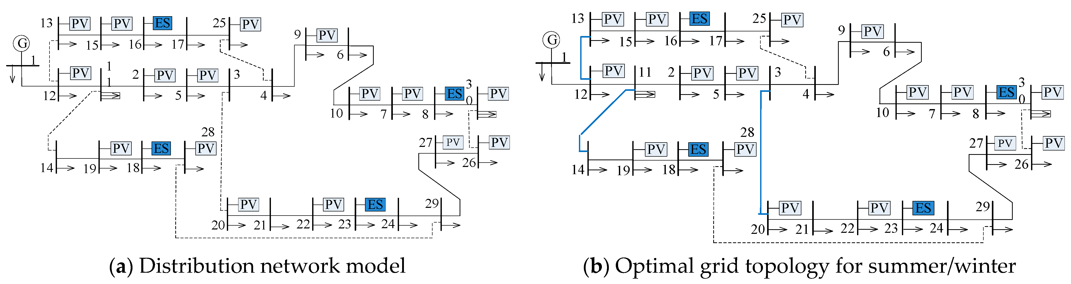
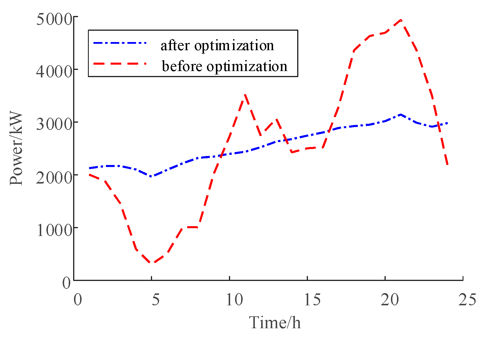
Considering the large-scale grid connection of distributed PV, the fixed grid topology cannot realize the optimal operation of the distribution network. In this paper, the grid structure is optimized by reasonably opening and closing the tie lines, and the distribution of node voltage and grid power flow is improved. The ES charging and discharging power, controllable load power, and PV reactive power are optimized by hierarchical optimization and adjustment of the grid topology, which reduces grid losses and power fluctuations on the pulling lines.
(2)
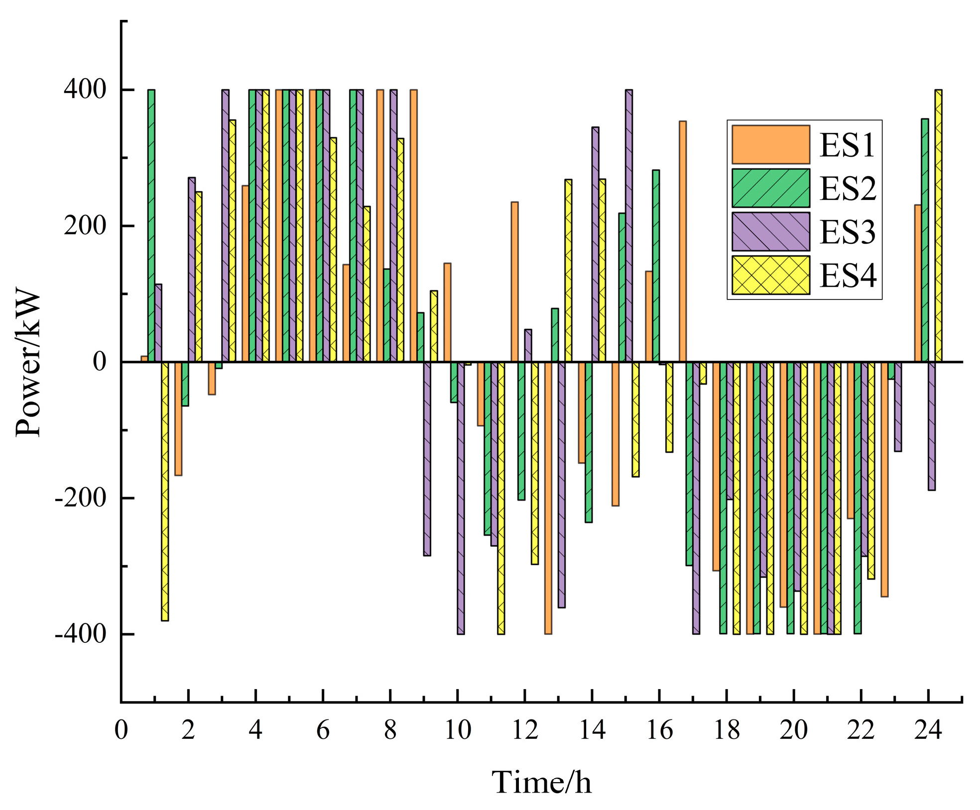
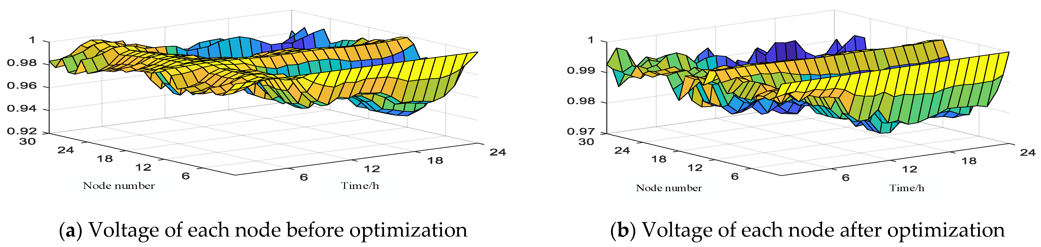
By adjusting the ES charging and discharging power and controllable load power, the fluctuation of tie-line power caused by the high proportion of distributed PV grid connections is reduced, grid loss is reduced, and the economic operation of the distribution network is achieved. The characteristics of the reactive power supply were fully utilized, its reactive output was rationally optimized, the node voltage amplitude was improved, and the voltage quality was enhanced.
(3)
The LM-IMCSDE algorithm improves the comprehensive performance of the algorithm based on the DE algorithm with the help of weighting Lehmer averages, improved multivariate collaboration, updated populations, and other strategies, as well as the algorithm test, which shows that the LM-IMCSDE algorithm has features such as faster convergence speed and stronger global search ability.
This research focuses on taking the typical scenario of a high proportion of distributed photovoltaic grid connections against the background. This paper constructs an optimal scheduling model in distribution networks, considering their adjustment potential to fulfil grid requirements. However, it is essential to acknowledge certain limitations within this study, as the scope remains constrained to specific research objectives. In future research, the relevant work will be further refined and improved, such as excavating the flexible adjustment capacity of system and framework planning schemes, as well as system operation strategies under multiple time scales.

Author Contributions

T.Z.: Methodology, Software, Writing-Original draft preparation, Writing-Reviewing and Editing. X.Z.: Data curation, Investigation. Y.G.: Conceptualization, Validation, Supervision. R.Z.: Visualization, Investigation. All authors have read and agreed to the published version of the manuscript.

Funding

This research was funded by the Tibet Autonomous Region Natural Science Key Project Fund Key Project (XZ202201ZR0024G), the National Natural Science Foundation of China (52167015), and Tibet Autonomous Region Education Department Key Laboratory of Colleges and Universities-Electrical Engineering Laboratory Support Project (2022D-ZN-01).

Data Availability Statement

Not applicable.

Acknowledgments

This work was supported by the Tibet Autonomous Region Natural Science Key Project Fund (XZ202201ZR0024G), the National Natural Science Foundation of China (52167015), and Tibet Autonomous Region Education Department Key Laboratory of Colleges and Universities-Electrical Engineering Laboratory Support Project (2022D-ZN-01).

Conflicts of Interest

The authors declare that they have no known competing financial interests or personal relationships that could have appeared to influence the work reported in this paper.

References

  1. Pingkuo, L.; Zhongfu, T. How to develop distributed generation in China: In the context of the reformation of electric power system. Renew. Sustain. Energy Rev. 2016, 66, 10–26. [Google Scholar] [CrossRef]
  2. Cai, Y.; Yang, A.; Chen, X.; Wen, X.; Fu, Y.; Xiao, X.; Li, Y. An Adaptive Control in a LV Distribution Network Integrating Distributed PV Systems by Considering Electricity Substitution. In Proceedings of the 2021 International Joint Conference on Energy, Electrical and Power Engineering; Springer: Singapore, 2022; pp. 277–296. [Google Scholar]
  3. İnci, M.; Savrun, M.M.; Çelik, Ö. Integrating electric vehicles as virtual power plants: A comprehensive review on vehicle-to-grid (V2G) concepts, interface topologies, marketing and future prospects. J. Energy Storage 2022, 55, 105579. [Google Scholar] [CrossRef]
  4. Jiang, X.; Wang, S.; Zhao, Q.; Wang, X. Exploiting the operational flexibility of AC-MTDC distribution system considering various flexible resources. Int. J. Electr. Power Energy Syst. 2023, 148, 108842. [Google Scholar]
  5. Deshpande, K.; Möhl, P.; Hämmerle, A.; Weichhart, G.; Zörrer, H.; Pichler, A. Energy management simulation with multi-agent reinforcement learning: An approach to achieve reliability and resilience. Energies 2022, 15, 7381. [Google Scholar] [CrossRef]
  6. Jani, A.; Karimi, H.; Jadid, S. Multi-time scale energy management of multi-microgrid systems considering energy storage systems: A multi-objective two-stage optimization framework. J. Energy Storage 2022, 51, 104554. [Google Scholar]
  7. Jani, A.; Karimi, H.; Jadid, S. Two-layer stochastic day-ahead and real-time energy management of networked microgrids considering integration of renewable energy resources. Appl. Energy 2022, 323, 119630. [Google Scholar] [CrossRef]
  8. Aljafari, B.; Vasantharaj, S.; Indragandhi, V.; Vaibhav, R. Optimization of DC, AC, and hybrid AC/DC microgrid-based IoT systems: A review. Energies 2022, 15, 6813. [Google Scholar] [CrossRef]
  9. Duan, J.; Liu, F.; Yang, Y. Optimal operation for integrated electricity and natural gas systems considering demand response uncertainties. Appl. Energy 2022, 323, 119455. [Google Scholar]
  10. Vermesan, O.; Friess, P.; Guillemin, P.; Serrano, M.; Bouraoui, M.; Freire, L.P.; Kallstenius, T.; Lam, K.; Eisenhauer, M.; Moessner, K.; et al. IoT digital value chain connecting research, innovation and deployment. In Digitising the Industry Internet of Things Connecting the Physical, Digital and VirtualWorlds; River Publishers: Chicago, IL, USA, 2022; pp. 15–128. [Google Scholar]
  11. Wang, Y.; Chen, X.; Dai, H. Comparative Study of Domestic and Foreign Urban Energy Internet Demonstration Practice. In Proceedings of the 2021 6th International Conference on Power and Renewable Energy (ICPRE), Shanghai, China, 17–20 September 2021; pp. 1409–1415. [Google Scholar]
  12. Mahmoodi, M.; Attarha, A.; Noori R, S.M.; Scott, P.; Blackhall, L. Adjustable robust approach to increase DG hosting capacity in active distribution systems. Electr. Power Syst. Res. 2022, 211, 108347. [Google Scholar] [CrossRef]
  13. Kuang, H.; Su, F.; Chang, Y.; Wang, K.; He, Z. Reactive power optimization for distribution network system with wind power based on improved multi-objective particle swarm optimization algorithm. Electr. Power Syst. Res. 2022, 213, 108731. [Google Scholar]
  14. Kaluthanthrige, R.; Rajapakse, A.D. Evaluation of hierarchical controls to manage power, energy and daily operation of remote off-grid power systems. Appl. Energy 2021, 299, 117259. [Google Scholar] [CrossRef]
  15. Wang, S.; Liu, Q.; Ji, X. A fast sensitivity method for determining line loss and node volt-ages in active distribution network. IEEE Trans. Power Syst. 2017, 33, 1148–1150. [Google Scholar] [CrossRef]
  16. Liu, Y.; Li, J.; Wu, L. Coordinated optimal network reconfiguration and voltage regulator/DER control for unbalanced distribu-tion systems. IEEE Trans. Smart Grid 2018, 10, 2912–2922. [Google Scholar]
  17. Sun, B.; Li, Y.; Zeng, Y.; Li, C.; Shi, J.; Ma, X. Distribution transformer cluster flexible dispatching method based on discrete monkey algorithm. Energy Rep. 2021, 7, 1930–1942. [Google Scholar] [CrossRef]
  18. Sun, B.; Jing, R.; Zeng, Y.; Li, Y.; Chen, J.; Liang, G. Distributed optimal dispatch-ing method for smart distribution network considering effective interaction of source-network-load-storage flexible resources. Energy Rep. 2023, 9, 148–162. [Google Scholar] [CrossRef]
  19. Wang, X.; Li, S.; Zhong, Y.; Li, C.; Lu, D.; Jia, K.; Liu, D.; Shi, F. Joint optimization of active/reactive power in the archipelago power grid with weak AC/multi-terminal flexible DC hybrid connection. Power Autom. Equip. 2020, 40, 132–137. (In Chinese) [Google Scholar]
  20. Xu, Z.; Huang, C. Reactive power optimization of distribution network with wind turbines in the electricity market environment. J. Power Syst. Autom. 2020, 32, 131–137. (In Chinese) [Google Scholar]
  21. Kumari, B.A.; Vaisakh, K. Integration of solar and flexible resources into expected security cost with dynamic optimal power flow problem using a novel DE algorithm. Renew. Energy Focus 2022, 42, 48–69. [Google Scholar] [CrossRef]
  22. Liu, H.; Qu, J.; Li, Y. The economic dispatch of wind integrated power system based on an improved differential evolution algorithm. Recent Adv. Electr. Electron. Eng. (Former. Recent Pat. Electr. Electron. Eng.) 2020, 13, 384–395. [Google Scholar] [CrossRef]
  23. Chi, R.; Li, Z.; Chi, X.; Qu, Z.; Tu, H. Reactive power optimization of power system based on improved differential evolution algorithm. Math. Probl. Eng. 2021, 2021, 1–19. [Google Scholar] [CrossRef]
  24. Li, Y.; Sun, B.; Zeng, Y.; Dong, S.; Ma, S.; Zhang, X. Active distribution network active and reactive power coordinated dispatching method based on discrete monkey algorithm. Int. J. Electr. Power Energy Syst. 2022, 143, 108425. [Google Scholar] [CrossRef]
  25. El Sehiemy, R.A.; Selim, F.; Bentouati, B.; Abido, M. A novel multi-objective hybrid particle swarm and salp optimization algorithm for technical-economical-environmental operation in power systems. Energy 2020, 193, 116817. [Google Scholar] [CrossRef]
  26. Emre, Ç.; Nihat, Ö.; Houssein Essam, H. Influence of energy storage device on load frequency control of an interconnected dual-area thermal and solar photovoltaic power system. Neural Comput. Appl. 2022, 34, 20083–20099. [Google Scholar]
  27. Hou, J.; Yu, W.; Xu, Z.; Ge, Q.; Li, Z.; Meng, Y. Multi-time scale optimization scheduling of microgrid considering source and load uncertainty. Electr. Power Syst. Res. 2023, 216, 109037. [Google Scholar] [CrossRef]
Figure 1. Hierarchical optimization framework diagram.
Processes 11 02824 g001
Figure 2. Function test comparison diagram.
Processes 11 02824 g002
Figure 3. IEEE’s typical distribution network model.
Processes 11 02824 g003
Figure 4. Typical daily power chart in summer.
Processes 11 02824 g004
Figure 5. Typical daily power chart in winter.
Processes 11 02824 g005
Figure 6. ES charging and discharging power.
Processes 11 02824 g006
Figure 7. Voltage of each node before and after optimization.
Processes 11 02824 g007
Figure 8. Power of the tie line before and after optimization.
Processes 11 02824 g008
Figure 9. Grid loss before and after optimization.
Processes 11 02824 g009
Figure 10. ES charging and discharging power.
Processes 11 02824 g010
Figure 11. Voltage of each node before and after optimization.
Processes 11 02824 g011
Figure 12. Power of the tie line before and after optimization.
Processes 11 02824 g012
Figure 13. Grid loss before and after optimization.
Processes 11 02824 g013
Table 1. Test function.
Function NameFunction
Griewank f ( x ) = 1 4000 i = 1 n x i 2 i n ( x i / x i ) + 1
Sphere f ( x ) = i n x i 2
Disclaimer/Publisher’s Note: The statements, opinions and data contained in all publications are solely those of the individual author(s) and contributor(s) and not of MDPI and/or the editor(s). MDPI and/or the editor(s) disclaim responsibility for any injury to people or property resulting from any ideas, methods, instructions or products referred to in the content.

