

A Fault Detection and Isolation Method via Shared Nearest Neighbor for Circulating Fluidized Bed Boiler

Abstract
:1. Introduction
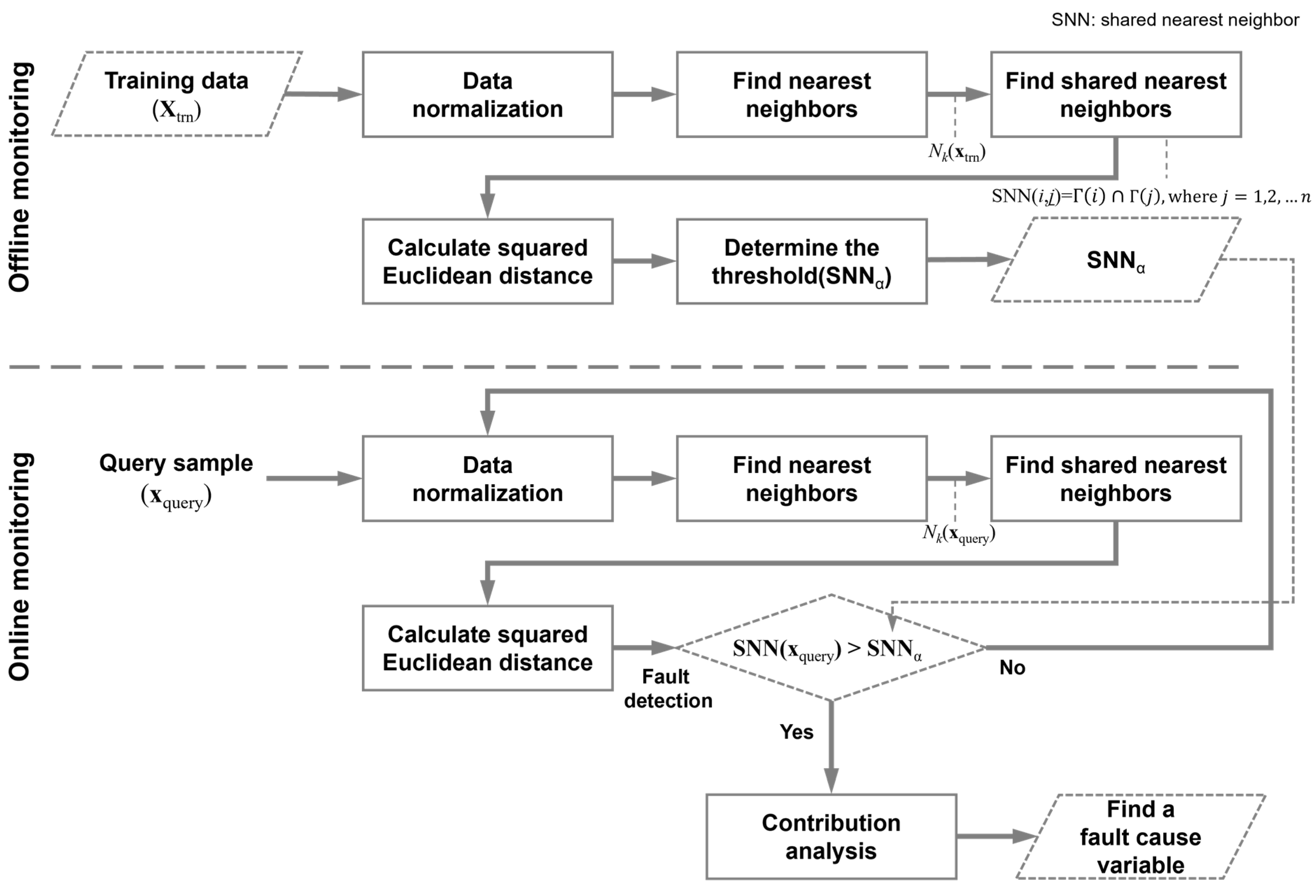
2. Proposed Method
2.1. Shared Nearest Neighbor
2.2. Nearest Neighbor Difference Normalization
- (1)
- To compute the NND, kNN is used to explore the nearest neighbors. The neighbors of a query vector are subtracted from the corresponding query vector to compute the first-order NND, as shown in Equation (4):where and denote the nearest neighbors of the training data and query vectors, respectively. The first-order NND, computed using Equation (4), removes the multicenter structure, while preserving the position information between the current sample and its nearest neighbors.
- (2)
- Subsequently, the second-order NND was calculated to convert the multimode data into single-mode data, as shown in Equation (5):where denotes a weight parameter used to map to a single mode. is the Euclidean distance between the query vector and the kth neighbor training data. The original data are converted into a single mode with multiple modes using a second-order NND. In addition, after the second-order NND, each variable follows a multivariate Gaussian distribution. A detailed explanation of how multimode characteristics are removed using NND can be found in [1]. In this study, a SNN was applied to data from which multimode characteristics were removed to calculate the detection index for identifying failure variables.
3. Numerical Simulation Study
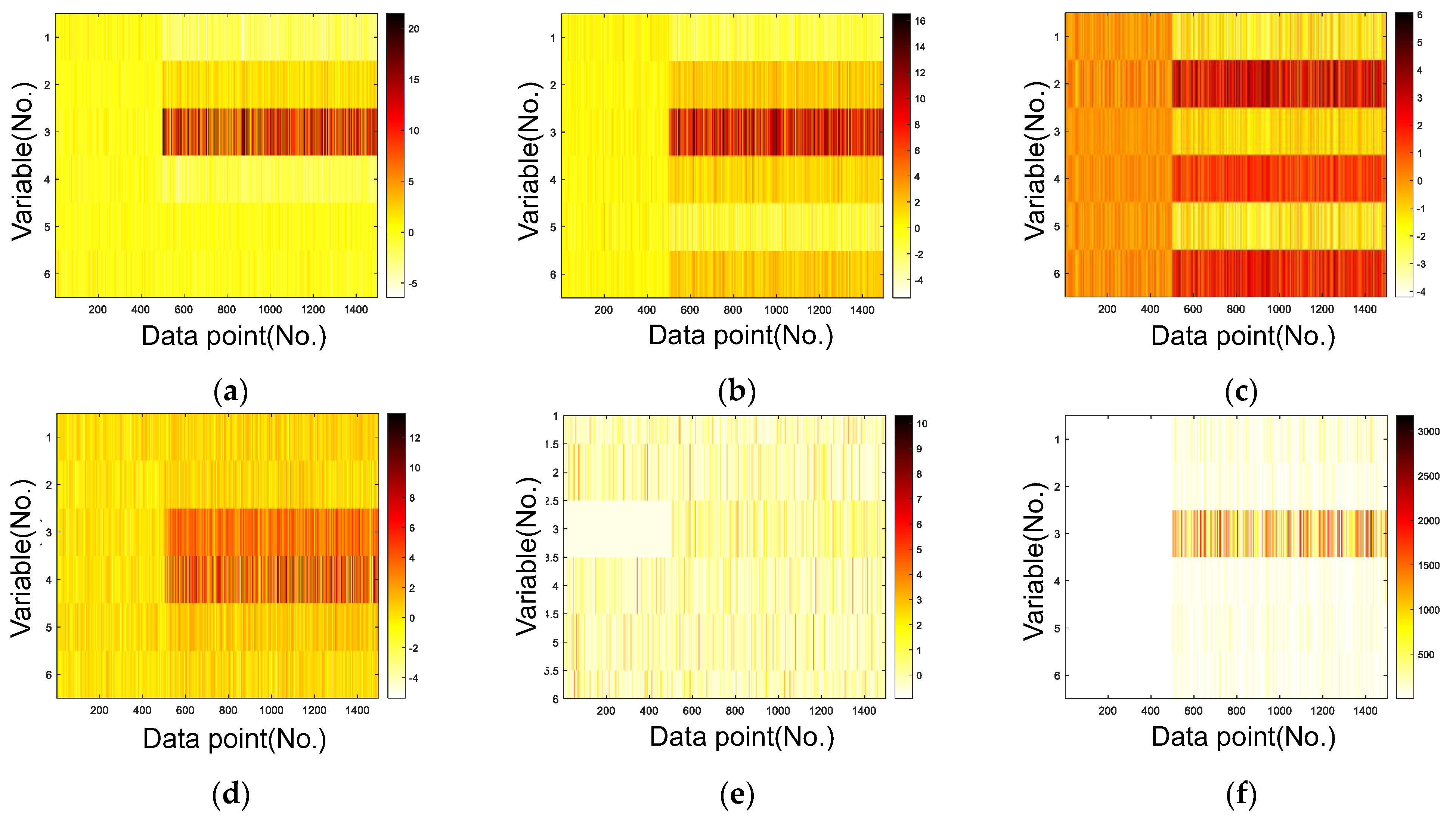
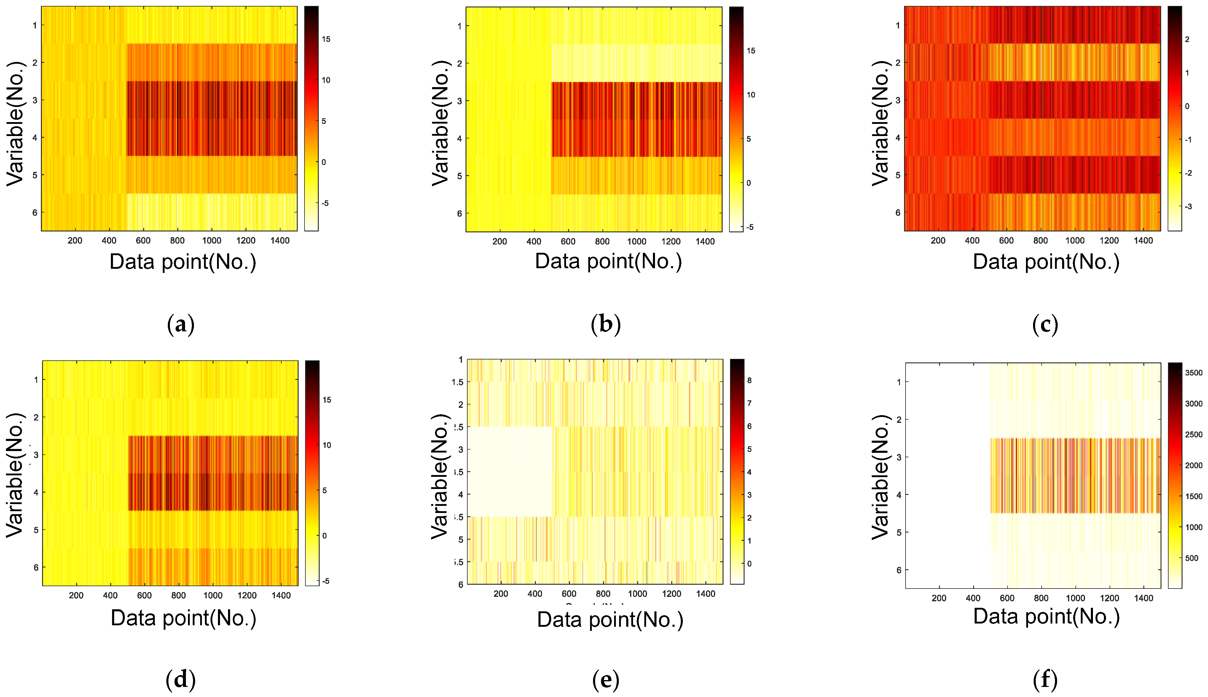
3.1. Multimode Numerical Example
- Case 1. The system was initially running normally, and then an arbitrary bias-type single fault was added from the 501st to the 1500th sample.
- Case 2. The system was initially running normally, and then arbitrary bias-type multiple faults were added from the 501st to 1500th samples.
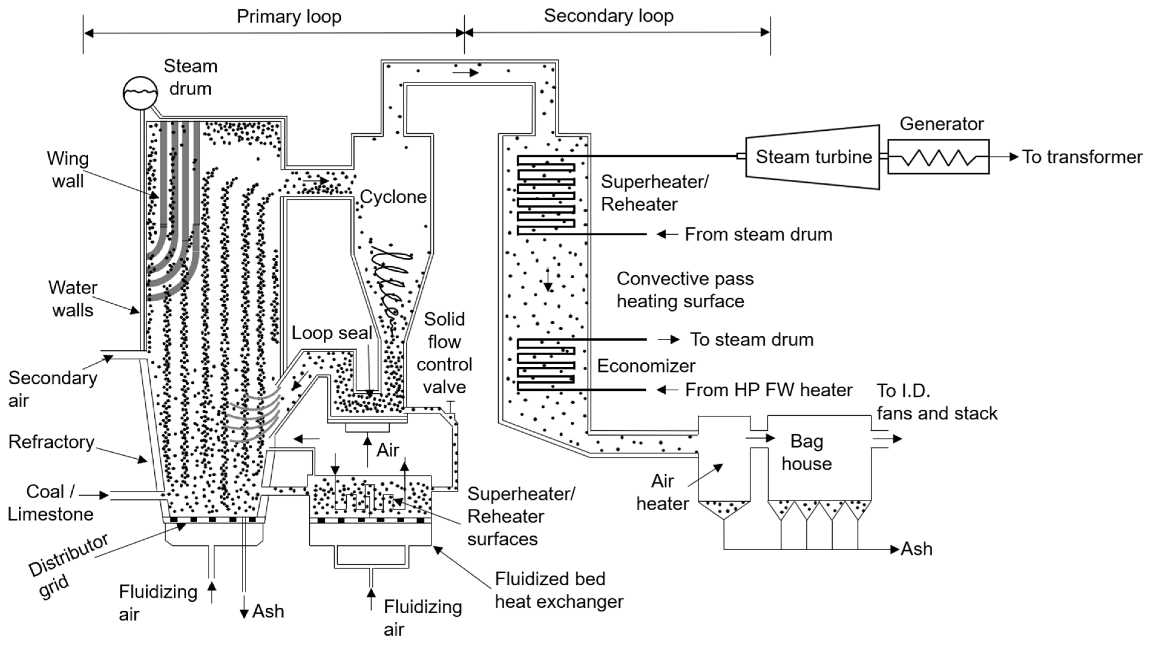
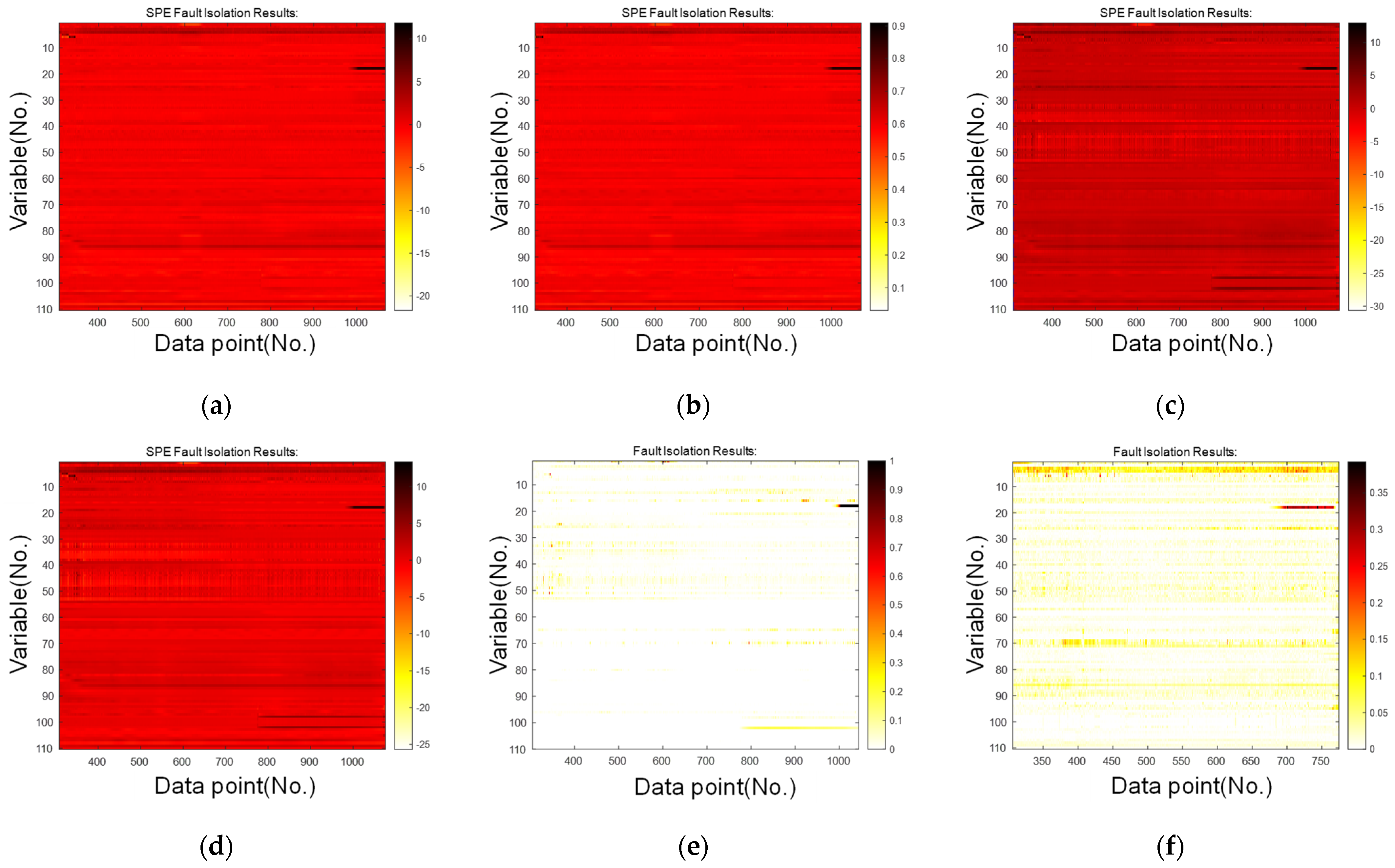
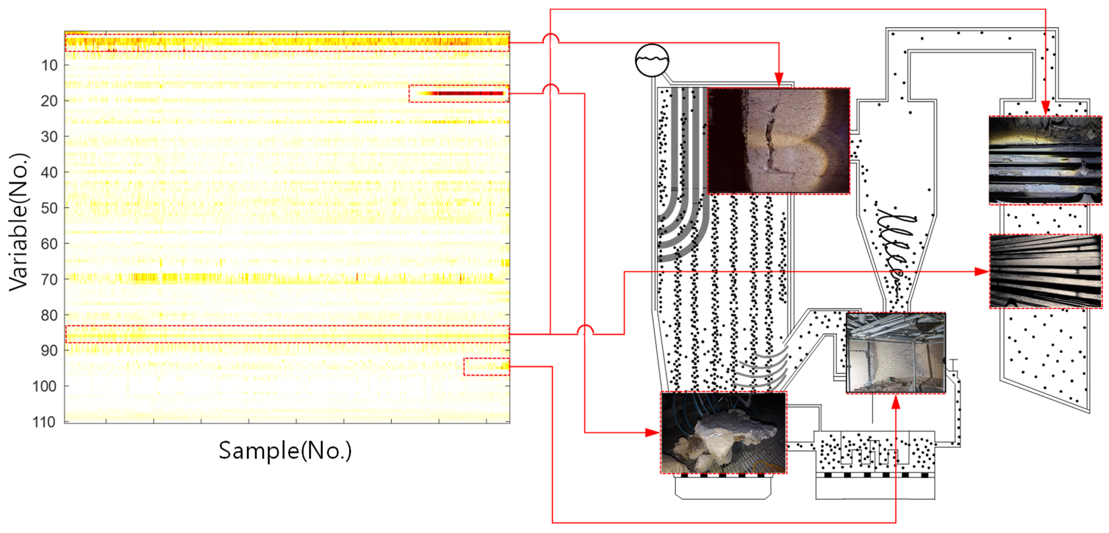
4. Actual Failure Case Study
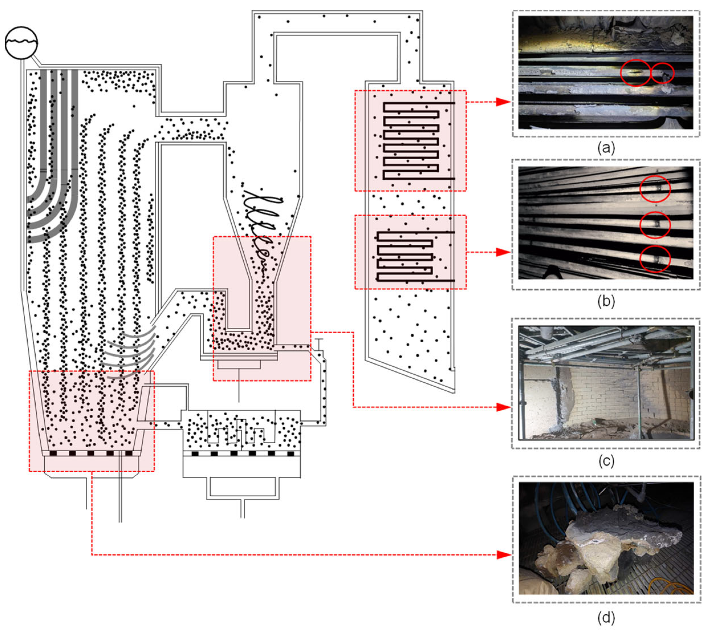
4.1. Circulating Fluidized Bed Boiler Structure
5. Conclusions
Author Contributions
Funding
Data Availability Statement
Conflicts of Interest
References
- Zhang, C.; Gao, X.; Xu, T.; Li, Y. Nearest neighbor difference rule–based kernel principal component analysis for fault detection in semiconductor manufacturing processes. J. Chemom. 2017, 31, e2888. [Google Scholar] [CrossRef]
- Guo, J.; Tangming, Y.; Yuan, L. Fault detection of multimode process based on local neighbor normalized matrix. Chemom. Intell. Lab. Syst. 2016, 154, 162–175. [Google Scholar] [CrossRef]
- Ge, Z.; Gao, F.; Song, Z. Two-dimensional Bayesian monitoring method for nonlinear multimode processes. Chem. Eng. Sci. 2011, 66, 5173–5183. [Google Scholar] [CrossRef]
- Jie, Y. A nonlinear kernel Gaussian mixture model based inferential monitoring approach for fault detection and diagnosis of chemical processes. Chem. Eng. Sci. 2012, 68, 506–519. [Google Scholar]
- Yu, J.; Jang, J.; Yoo, J.; Park, J.H.; Kim, S. Leakage detection of steam boiler tube in thermal power plant using principal component analysis. In Proceedings of the Annual Conference of the PHM Society 2016, Denver, CO, USA, 3–6 October 2016. [Google Scholar]
- Nomikos, P.; MacGregor, J.F. Multivariate SPC charts for monitoring batch processes. Technometrics 1995, 37, 41–59. [Google Scholar] [CrossRef]
- Wise, B.M.; Gallagher, N.B. The process chemometrics approach to process monitoring and fault detection. J. Process Control 1996, 6, 329–348. [Google Scholar] [CrossRef]
- Ali, A.; Daneshvar, M. Data driven approach for fault detection and diagnosis of turbine in thermal power plant using Independent Component Analysis (ICA). Int. J. Electr. Power Energy Syst. 2011, 43, 728–735. [Google Scholar]
- Chun-Chin, H.; Su, C.-T. An adaptive forecast-based chart for non-Gaussian processes monitoring: With application to equipment malfunctions detection in a thermal power plant. IEEE Trans. Control Syst. Technol. 2010, 19, 1245–1250. [Google Scholar]
- Wang, G.; Liu, J.; Zhang, Y.; Li, Y. A novel multi-mode data processing method and its application in industrial process monitoring. J. Chemom. 2015, 29, 126–138. [Google Scholar] [CrossRef]
- Yu, J.; Jang, J.; Yoo, J.; Park, J.H.; Kim, S. A fault isolation method via classification and regression tree-based variable ranking for drum-type steam boiler in thermal power plant. Energies 2018, 11, 1142. [Google Scholar] [CrossRef]
- Westerhuis, J.A.; Gurden, S.P.; Smilde, A.K. Generalized contribution plots in multivariate statistical process monitoring. Chemom. Intell. Lab. Syst. 2000, 51, 95–114. [Google Scholar] [CrossRef]
- Conlin, A.K.; Martin, E.B.; Morris, A.J. Confidence limits for contribution plots. J. Chemom. 2000, 14, 725–736. [Google Scholar] [CrossRef]
- Alcala, C.F.; Qin, S.J. Reconstruction-based contribution for process monitoring. Automatica 2009, 45, 1593–1600. [Google Scholar] [CrossRef]
- Alcala, C.F.; Qin, S.J. Analysis and generalization of fault diagnosis methods for process monitoring. J. Process Control 2011, 21, 322–330. [Google Scholar] [CrossRef]
- Kourti, T.; MacGregor, J.F. Multivariate SPC methods for process and product monitoring. J. Qual. Technol. 1996, 28, 409–428. [Google Scholar] [CrossRef]
- Liu, J. Fault diagnosis using contribution plots without smearing effect on non-faulty variables. J. Process Control 2012, 22, 1609–1623. [Google Scholar]
- Zhou, Z.; Wen, C.; Yang, C. Fault isolation based on k-nearest neighbor rule for industrial processes. IEEE Trans. Ind. Electron. 2016, 63, 2578–2586. [Google Scholar] [CrossRef]
- Xu, H.; Yang, F.; Ye, H.; Li, W.; Xu, P.; Usadi, A.K. Weighted reconstruction-based contribution for improved fault diagnosis. Ind. Eng. Chem. Res. 2013, 52, 9858–9870. [Google Scholar] [CrossRef]
- Wang, G.; Liu, J.; Li, Y. Fault diagnosis using kNN reconstruction on MRI variables. J. Chemom. 2015, 29, 399–410. [Google Scholar] [CrossRef]
- Zhang, L.; Lin, J.; Karim, R. Sliding window-based fault detection from high-dimensional data streams. IEEE Trans. Syst. Man Cybern. Syst. 2016, 47, 289–303. [Google Scholar] [CrossRef]
- Guo, J.; Wang, X.; Li, Y. kNN based on probability density for fault detection in multimodal processes. J. Chemom. 2018, 32, e3021. [Google Scholar] [CrossRef]
- Basu, S.; Debnath, A.K. Power Plant Instrumentation and Control Handbook: A Guide to Thermal Power Plants; Academic Press: Cambridge, MA, USA, 2014. [Google Scholar]
- Öngelen, G.; İnkaya, T. LOF weighted KNN regression ensemble and its application to a die manufacturing company. Sādhanā 2023, 48, 246. [Google Scholar] [CrossRef]
- Rostek, K.; Morytko, Ł.; Jankowska, A. Early detection and prediction of leaks in fluidized-bed boilers using artificial neural networks. Energy 2015, 89, 914–923. [Google Scholar] [CrossRef]
- Van Caneghem, J.; Brems, A.; Lievens, P.; Block, C.; Billen, P.; Vermeulen, I.; Dewil, R.; Baeyens, J.; Vandecastelle, C. Fluidized bed waste incinerators: Design, operational and environmental issues. Prog. Energy Combust. Sci. 2012, 38, 551–582. [Google Scholar] [CrossRef]
- Obernberger, I. Decentralized biomass combustion: State of the art and future development. Biomass Bioenergy 1998, 14, 33–56. [Google Scholar] [CrossRef]
- Khan, A.A.; de Jong, W.; Jansens, P.J.; Spliethoff, H. Biomass combustion in fluidized bed boilers: Potential problems and remedies. Fuel Process. Technol. 2009, 90, 21–50. [Google Scholar] [CrossRef]
- Kim, M.; Jung, S.; Kim, B.; Kim, J.; Kim, E.; Kim, J.; Kim, S. Fault Detection Method via k-Nearest Neighbor Normalization and Weight Local Outlier Factor for Circulating Fluidized Bed Boiler with Multimode Process. Energies 2022, 15, 6146. [Google Scholar] [CrossRef]
- Li, Y.S.; Sanchez-Pasten, M.; Spiegel, M. High temperature interaction of pure Cr with KCl. Mater. Sci. Forum 2004, 461, 1047–1054. [Google Scholar] [CrossRef]
- Oka, S. Fluidized Bed Combustion; CRC Press: Boca Raton, FL, USA, 2003. [Google Scholar]
- Huang, C.-C.; Chen, T.; Yao, Y. Mixture Discriminant Monitoring: A Hybrid Method for Statistical Process Monitoring and Fault Diagnosis/Isolation. Ind. Chem. Res. 2013, 52, 10720–10731. [Google Scholar] [CrossRef]
- Dai, X.; Gao, Z. From model, signal to knowledge: A data-driven perspective of fault detection and diagnosis. IEEE Trans. Ind. Inform. 2013, 9, 2226–2238. [Google Scholar] [CrossRef]
- Zhong, S.; Langseth, H.; Nielsen, T.D. A classification-based approach to monitoring the safety of dynamic systems. Reliab. Eng. Syst. Saf. 2014, 121, 61–71. [Google Scholar] [CrossRef]


| Method | PCA (SPE) | DPCA (SPE) | ICA (SPE) | DICA (SPE) | LOF (LOF) | SNN (D2) |
|---|---|---|---|---|---|---|
| FAR | FAR | FAR | FAR | FAR | FAR | |
| Single fault | 10.2 | 6.93 | 25 | 2.2 | 26.1 | 0 |
| Multiple fault | 6.93 | 2.53 | 48.7 | 0.4 | 15.1 | 0 |
| No. | Description | Unit | No. | Description | Unit | No. | Description | Unit |
|---|---|---|---|---|---|---|---|---|
| x1 | Amount of H2O | % | x38 | Steam press. of SCR | mmH2O | x75 | Inlet temp. inlet of upper place furnace | °C |
| x2 | Amount of O2 in eco. | % | x39 | Press. of steam supplied of upper place furnace | MPa | x76 | Inlet temp. inlet of furnace | °C |
| x3 | Diff. of press. furnace and top of cy. | mmH2O | x40 | Combustor bed press. of lower furnace feedwater (sensor A) | mmH2O | x77 | Inlet temp. inlet of cyclone and boiler front-end | °C |
| x4 | Diff. of press. 2nd and 1st S/H. | mmH2O | x41 | Combustor bed press. of lower furnace feedwater (sensor B) | mmH2O | x78 | Inlet temp. inlet of cyclone and boiler terminal | °C |
| x5 | Diff. of press. 1st S/H and 2nd eco. | mmH2O | x42 | Press. of lower place furnace | mmH2O | x79 | Diff. of temp. 2nd and 1st S/H | °C |
| x6 | Diff. of press. 2nd and 1st eco. | mmH2O | x43 | Press. of middle place furnace | mmH2O | x80 | Inlet temp. inlet of 1st S/H | °C |
| x7 | Diff. of press. of 1st and new eco. | mmH2O | x44 | Press. of upper place furnace | mmH2O | x81 | Diff. of temp. 1st S/H and 2nd eco. | °C |
| x8 | Diff. of press. of new eco. | mmH2O | x45 | Press. between cyclone and boiler | mmH2O | x82 | Inlet temp. inlet of 2nd S/H | °C |
| x9 | Output of steam ratio (sensor A) | % | x46 | Press. of 1st S/H | mmH2O | x83 | Diff. of temp. 2nd and 1st eco. | °C |
| x10 | Output of steam ratio (sensor B) | % | x47 | Press. of 2nd economizer | mmH2O | x84 | Inlet temp. inlet of 1st eco. | °C |
| x11 | Output of steam ratio (sensor C) | % | x48 | Press. of Air pre-heater | mmH2O | x85 | Diff. of temp. 1st S/H and new eco. | °C |
| x12 | Steam output of feedwater pipe 1(sensor A) | t/h | x49 | Press. of lower supply cyclone (sensor A) | mmH2O | x86 | Inlet temp. inlet of 2nd eco. | °C |
| x13 | Steam output of feedwater pipe 1(sensor B) | t/h | x50 | Press. of middle place cyclone | mmH2O | x87 | Diff. of temp. new eco. and bag filter | °C |
| x14 | Steam output of feedwater pipe 2 (sensor C) | t/h | x51 | Press. of middle place furnace | mmH2O | x88 | Outlet temp. of air pre-heater terminal | °C |
| x15 | Steam output of fluidized bed material supply | t/h | x52 | Press. of lower place furnace | mmH2O | x89 | Outlet temp. of dry reactor front-end | °C |
| x16 | Aux. steam output of lower feedwater pipe | t/h | x53 | Press. of dry reactor and bag filter | mmH2O | x90 | Diff. of temp. cyclone and boiler | °C |
| x17 | Inlet output of feedwater pipe 1 | % | x54 | Steam flow of air pre-heater and dry reactor | mmH2O | x91 | Inlet temp. of cyclone fluidized bed material supply | °C |
| x18 | Outlet output of feedwater pipe 1 | % | x55 | Output of feedwater ratio (sensor A) | % | x92 | Steam output of steam drum | t/h |
| x19 | Outlet output of feedwater pipe 2 | % | x56 | Output of feedwater ratio (sensor B) | % | x93 | Amount of outlet steam flow 2nd S/H | t/h |
| x20 | Steam flow of fluidized bed material supply | t/h | x57 | Inlet temp. of dry reactor and bag filter | °C | x94 | Amount of inlet steam flow 2nd S/H | t/h |
| x21 | Steam flow between feedwater pipe 1 and 2 | t/h | x58 | Inlet temp. of SCR and SGR | °C | x95 | Steam drum level of feedwater tank | mm |
| x22 | Steam flow between feedwater pipe 1 and 2 | t/h | x59 | Inlet temp. of SGR and combustor | °C | x96 | Steam drum level of eco. | t/h |
| x23 | Metering bin A outlet conveyor | rpm | x60 | Outlet temp. of feedwater pipe 1 | °C | x97 | Outlet press. of 2nd S/H 1-1 | MPa |
| x24 | Diff. press. between feedwater pipe 1 | mmH2O | x61 | Outlet temp. of feedwater pipe 2 | °C | x98 | Outlet press. 2nd S/H | MPa |
| x25 | Diff. press. of feedwater pipe 1 (sensor A and B) | mmH2O | x62 | Outlet temp. of upper place furnace | °C | x99 | Inlet press. 2nd S/H | MPa |
| x26 | Diff. press. between dry reactor and bag filter | mmH2O | x63 | Inlet temp. inlet of cyclone and boiler middle point | °C | x100 | Outlet press. steam supplied of 2nd S/H | MPa |
| x27 | Sum of steam output of feedwater pipe 1 and 2 | mmH2O | x64 | Outlet temp. of upper place boiler | °C | x101 | Outlet press. of 2nd S/H 1-1 | MPa |
| x28 | Furnace press. of feedwater pipe 2 | mmH2O | x65 | Inlet temp. of feedwater pipe 1 (sensor B) | °C | x102 | Temp. of steam supplied of boiler silencer | °C |
| x29 | Furnace press. of feedwater pipe 2 (sensor A) | mmH2O | x66 | Inlet temp. of feedwater pipe 2 (sensor B) | °C | x103 | Outlet temp. of 1st S/H | °C |
| x30 | Furnace press. of feedwater pipe (sensor B) | mmH2O | x67 | Inlet temp. of feedwater pipe 1 | °C | x104 | Temp. of steam supplied of boiler silencer | °C |
| x31 | Press. of fluidized bed material supply | mmH2O | x68 | Inlet temp. of feedwater pipe 2 | °C | x105 | Output of steam drum | % |
| x32 | Press. of 2nd S/H | mmH2O | x69 | Inlet temp. of feedwater pipe 1 (sensor A) | °C | x106 | Outlet temp. of 1st S/H | °C |
| x33 | Press. of lower supply cyclone (sensor B) | mmH2O | x70 | Inlet temp. of feedwater pipe 1 (sensor A) | °C | x107 | Inlet temp. of 2nd S/H (sensor A) | °C |
| x34 | Inlet press. of feedwater pipe 2 | mmH2O | x71 | Inlet temp. of feedwater pipe 2 (sensor A) | °C | x108 | Inlet temp. of 2nd S/H (sensor B) | °C |
| x35 | Press. of air pre-heater and dry reactor | mmH2O | x72 | Inlet temp. inlet of fluidized bed material supply | °C | x109 | Inlet temp. of 1st S/H (sensor A) | °C |
| x36 | Press of upper place combustor | mmH2O | x73 | Inlet temp. inlet of lower place furnace (sensor A) | °C | x110 | Inlet temp. of 1st S/H (sensor B) | °C |
| x37 | Press. of SCR terminal | mmH2O | x74 | Inlet temp. inlet of lower place furnace (sensor B) | °C |
| PCA | DPCA | ICA | DICA | LOF | SNN | |
|---|---|---|---|---|---|---|
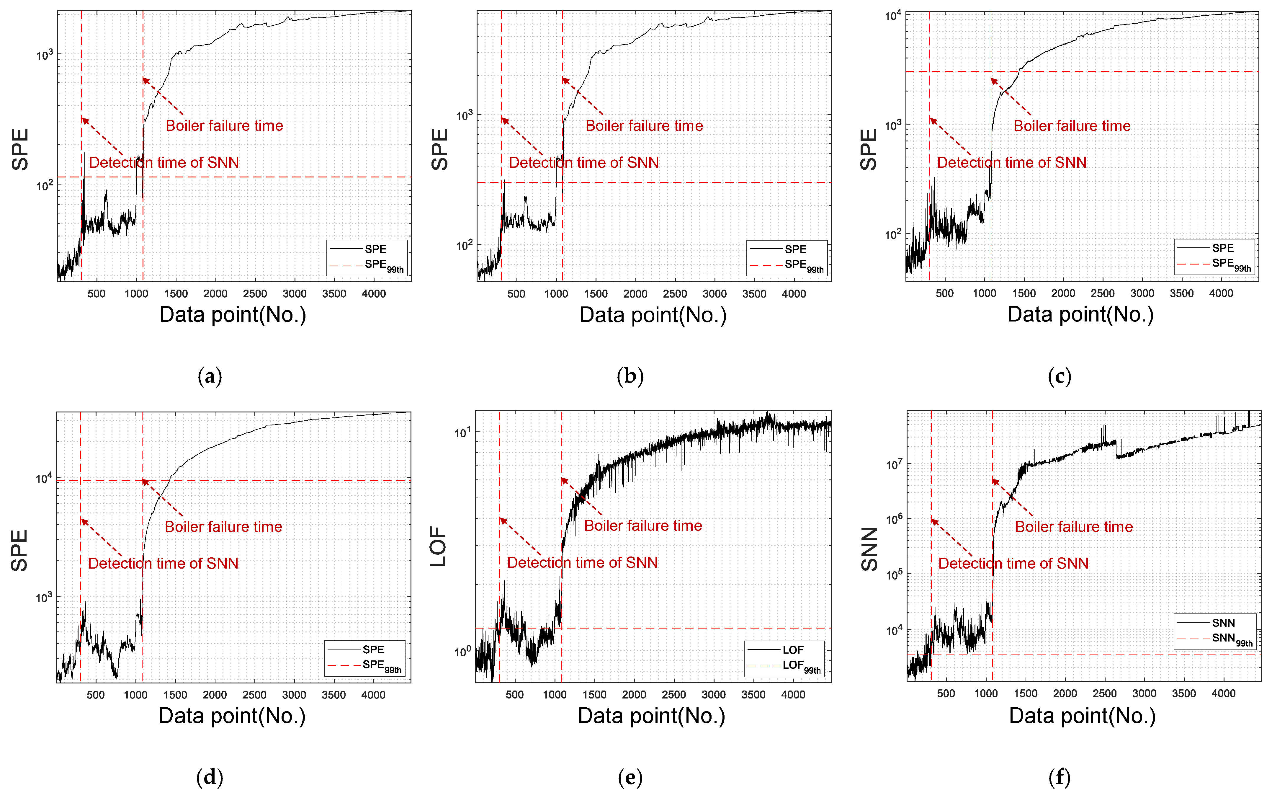
| Failure time | 14 h 35 m 6 s | |||||
| Detection time | 14 h 34 m | 14 h 27 m | - | - | 14 h 20 m | 12 h 26 m |
| Early detection time | 1 m ago | 28 m 40 s ago | - | - | 14 m 16 s ago | 2 h 9 m ago |
Disclaimer/Publisher’s Note: The statements, opinions and data contained in all publications are solely those of the individual author(s) and contributor(s) and not of MDPI and/or the editor(s). MDPI and/or the editor(s) disclaim responsibility for any injury to people or property resulting from any ideas, methods, instructions or products referred to in the content. |
© 2023 by the authors. Licensee MDPI, Basel, Switzerland. This article is an open access article distributed under the terms and conditions of the Creative Commons Attribution (CC BY) license (https://creativecommons.org/licenses/by/4.0/).
Share and Cite
Kim, M.; Jung, S.; Kim, E.; Kim, B.; Kim, J.; Kim, S. A Fault Detection and Isolation Method via Shared Nearest Neighbor for Circulating Fluidized Bed Boiler. Processes 2023, 11, 3433. https://doi.org/10.3390/pr11123433
Kim M, Jung S, Kim E, Kim B, Kim J, Kim S. A Fault Detection and Isolation Method via Shared Nearest Neighbor for Circulating Fluidized Bed Boiler. Processes. 2023; 11(12):3433. https://doi.org/10.3390/pr11123433
Chicago/Turabian StyleKim, Minseok, Seunghwan Jung, Eunkyeong Kim, Baekcheon Kim, Jinyong Kim, and Sungshin Kim. 2023. "A Fault Detection and Isolation Method via Shared Nearest Neighbor for Circulating Fluidized Bed Boiler" Processes 11, no. 12: 3433. https://doi.org/10.3390/pr11123433