Investigating the Impact of Operating Conditions on Relief Pressure Valve Flow through CFD and Statistical Analysis

Abstract

This paper presents a comprehensive computational fluid dynamics (CFD) analysis of air/water flow through a discharge valve, focusing on four different seat–valve distances and three adjustment nozzle positions. The study investigates the velocity distribution, pressure profiles, tangential stresses, and turbulent kinetic energy within the valve and analyzes its performance under various operating conditions. Notably, peak velocities of 3210 m/s were observed between the valve seat and valve, with significant variations for different nozzle positions. Extreme pressure values centered on the valve plate, reaching 4.3 MPa. Tangential stresses were highest on the chamfered plate surface and varied on the seat, turbulent kinetic energy (TKE) exhibited randomness. This study provides valuable information for enhancing the valve’s efficiency in a wide range of industrial applications.

1. Introduction

Effective fluid flow control is a fundamental requirement in a wide array of industrial processes, where precision and efficiency are predominant. Within this context, discharge valves play a pivotal role in regulating fluid flow within pipelines and systems. A comprehensive understanding of airflow dynamics within these valves is essential for their optimal design and operation.

The stability of safety relief valves, essential for their reliable performance is influenced by various factors, such as the design of the valve, spring pre-deformation, the length of the inlet pipeline, valve opening length, the position of regulator rings and the volume of the pressure vessel [1].

Dasgupta and Karmakar [2] conducted research on the dynamics of a pilot-operated pressure relief valve using the Bondgraph simulation technique. They derived the governing equations of the system from their model and, in the process of numerically solving these equations, they considered the different pressure-flow characteristics of the valve ports. The simulation study identified specific critical design parameters that exerted a substantial impact on the transient response of the system. Similarly, Prescott and Ulanicki [3] created a straightforward highly precise model for analyzing the dynamic behavior of a pressure reducing valve. The primary contributions of their work included the formulation of multiple dynamic models, encompassing two phenomenological models, one behavioral model, and one linear model, all designed to effectively describe the functioning of pressure reducing valves.

Advancements in computational techniques have made it increasingly practical to analyze the intricate flow patterns within valves [4,5,6]. As a result, there has been a significant increase in research related to the functionality and design of valves [4,5,6,7,8,9,10,11].

The study [7] develops a numerical model using advanced computational fluid dynamics techniques to analyze a direct-operated safety relief valve. The model accurately simulates the entire process from valve opening to closure, providing insights into compressible fluid flow and the effects of design parameters.

A three-dimensional numerical analysis with CFD was performed in [1] to examine a safety relief valve’s performance under various conditions, including different openings and inlet pressures. The study compared mass flow and discharge coefficients from simulations with ASME 2011a Section 1 standards and the model proved consistent for openings below 12 mm and closely matched the ASME standard. Additionally, CFD simulations revealed that the average normal disc force was approximately 19% lower than the theoretical ASME force, which could help prevent valve oversizing.

A simplified dynamic model (based on the equation of motion for a single degree of freedom system, with the assumption that damping effects are negligible due to their minimal impact on reclosing time) was developed in [12] to predict the dynamic behavior during both the reclosing and blowdown phases of a conventional pressure relief valve. The study introduces a novel approach by integrating static computational fluid dynamics (CFD) analysis results, calculating the lift force coefficient of the valve at various fixed lift positions using static CFD analysis and then incorporates these values into the simplified dynamic model as the inherent characteristics of the valve.

CFD simulation was also used by Erdődi and Hős [13] to explore the dynamic instability (flutter/chatter) of gas-service direct spring operated pressure relief valves, specifically focusing on the acoustic coupling between the valve body dynamics and the upstream piping. To enhance accuracy and enable analytical computations, the paper introduces two CFD-based methods. The first involves steady-state CFD runs to validate and improve the reduced-order models. The second employs dynamic CFD simulations with deforming mesh technology, providing a high-fidelity resolution of valve response and transient fluid–structure interactions. Comparing results from both approaches validates the use of reduced-order models for stability predictions.

The scientific work [14] focused on the design and modeling of a buffer relief valve using ANSYS 2021 R1 software, in order to achieve an optimized design for this valve. The findings revealed a high level of agreement between the results obtained from ANSYS simulations and the actual experimental results, affirming that the valve is suitable and safe for operation at a pressure rating of 0.14 MpPa.

Hos et al. (2014) [15] conducted a study that both summarized and expanded upon recent scientific investigations into the causes of instability in pressure relief valves. The primary objective was to obtain a deeper and more comprehensive understanding of the factors influencing the stability of pressure relief valves during their operation. The authors specifically focused on direct spring-loaded pressure relief valves used in gas applications, with a particular emphasis on how valve dynamics interact with acoustic pressure waves in the inlet pipe, considering their combined effect on valve stability.

The paper [16] offers a comprehensive analysis of experimental findings concerning the static and dynamic behavior of a hydraulic pressure relief valve, specifically focusing on the factors that influence valve instability. The study reveals that both signals exhibit similar frequency content, and the frequency of chatter remains relatively constant over various parameter ranges, such as fluid velocity and set pressure. The paper also delineates different motion patterns, including stable operation, free motion, impacting oscillations, and chaotic behavior, as they relate to the interplay between fluid velocity and set pressure.

A model that captures the dynamic response of a pressure relief valve in gas or vapor service is introduced by Darby [17], taking into account a range of influencing factors. The model allows the prediction of the valve disk’s position over time, considering specific valve characteristics, operational conditions, and installation parameters. The model also incorporates the impact of these various parameters on the stability or instability of the valve disk’s response. Part II of the investigation program [18] presents an experimental testing program designed to investigate the opening stability of direct-acting pressure relief valves used in gas/vapor service, testing three different valve sizes from three manufacturers at two set pressures to assess their opening characteristics, specifically the relationship between disk lift and time. The tests varied the length of inlet piping and considered the presence or absence of discharge piping to identify conditions leading to unstable valve operation. Part III [19] includes a comparative analysis between the model’s predictions and the actual dynamic response data and also examines the details necessary for putting the model into practical use.

The article [10] aims to expand the understanding of self-excited oscillations in pressure relief valves through a combination of time history analysis, spectrogram post-processing, and experimental testing under various conditions. The study reveals the presence of low-frequency and high-frequency self-excited oscillations, identifying their potential causes, which include external vibrations and acoustic resonance in the vessel-pipe system, shedding light on the factors contributing to valve damage.

The scientific paper [20] gives important details regarding the utilization of Computational Fluid Dynamics (CFD) simulation techniques to analyze hydrodynamic phenomena within pipes, exploring various aspects related to the hydraulic efficiency of the pipe system.

On the other hand, external mechanical vibrations can disrupt the stability of valves when applied to their bodies. In such instances, vibrations are induced in the valve control element, such as the plug, ball, or spool [21]. Regarding this aspect, the work performed by Stosiak et al. [22] focuses on reducing the impact of external mechanical vibrations on hydraulic valves within various military hydraulic drive systems. The research explores the potential reduction of vibrations on the valve casing by incorporating flexibility into the valve installation on vibrating surfaces. This involves introducing materials with known stiffness and damping characteristics, such as steel spring packages or special cushions made of elastomer or oil-resistant rubber. Additionally, the study suggests that elastomer cushions within the valve casing, positioned between the casing and centering springs, can serve as a supplementary or alternative solution for dampening vibrations.

The primary focus of the present study centers on exploring the influence of four distinct seat–valve distances and three adjustment nozzle positions on flow characteristics within the valve. The novelty of this paper lies in its comprehensive investigation of the impact of seat–valve distances and adjustment nozzle positions on flow characteristics within the valve. The performed investigation explores parameters such as velocity distribution, pressure profiles, tangential stresses, and turbulent kinetic energy, providing a detailed understanding of how various operational conditions affect the valve’s performance.The practical application of this research is significant, as it offers valuable insights into optimizing the design and operation of these valves, the obtained results can be used to make informed decisions regarding seat–valve distances and adjustment nozzle positions, ultimately improving the efficiency and reliability of valves in real-world applications.

2. Materials and Methods

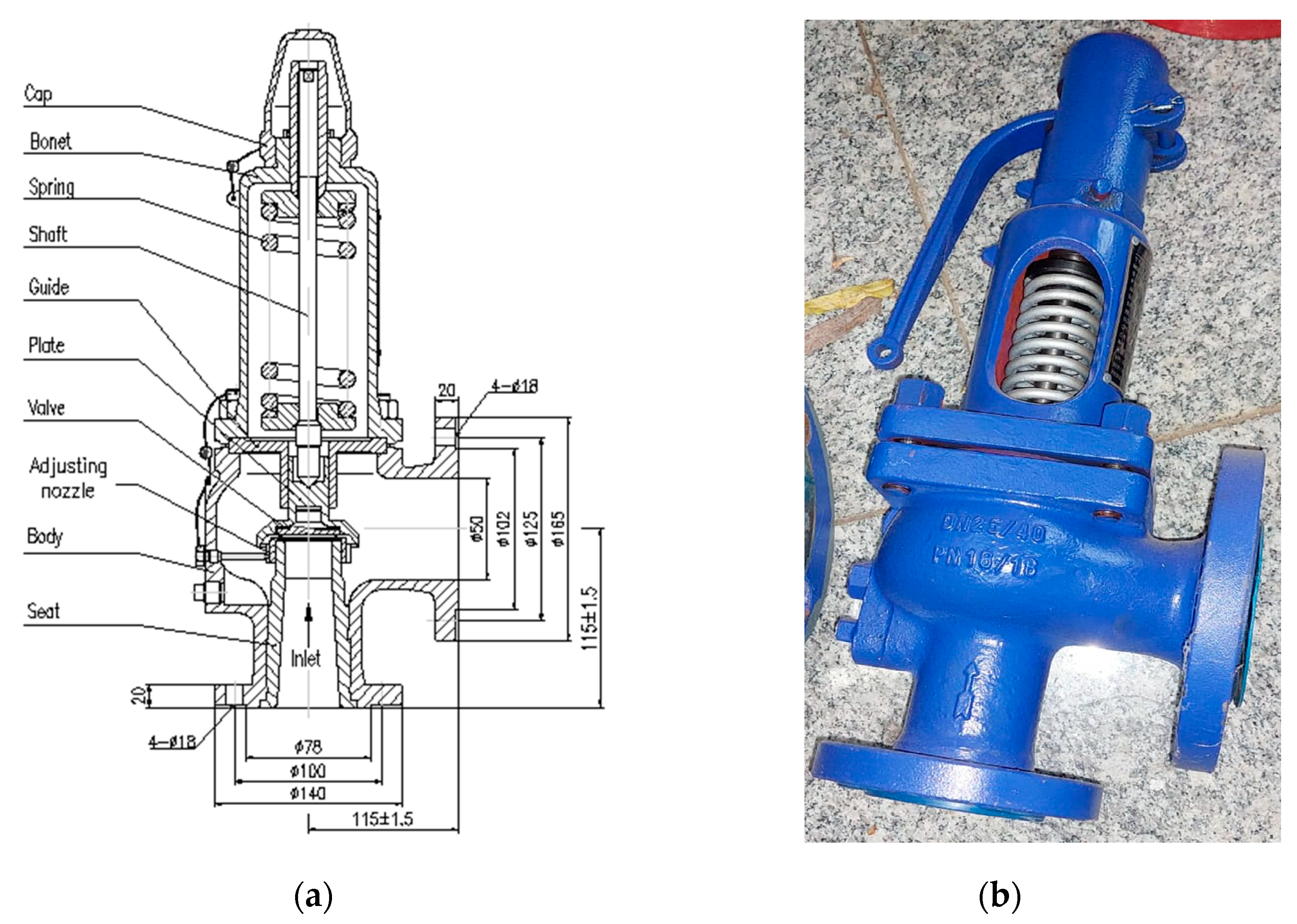
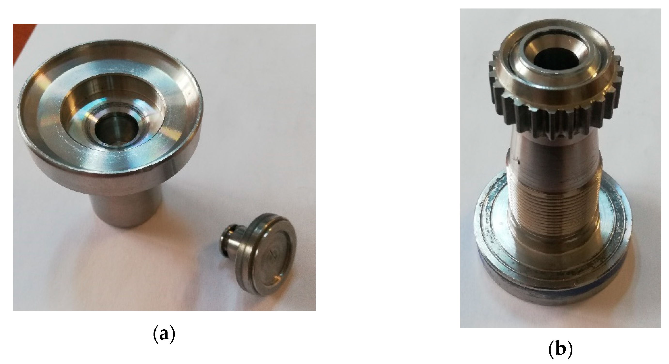
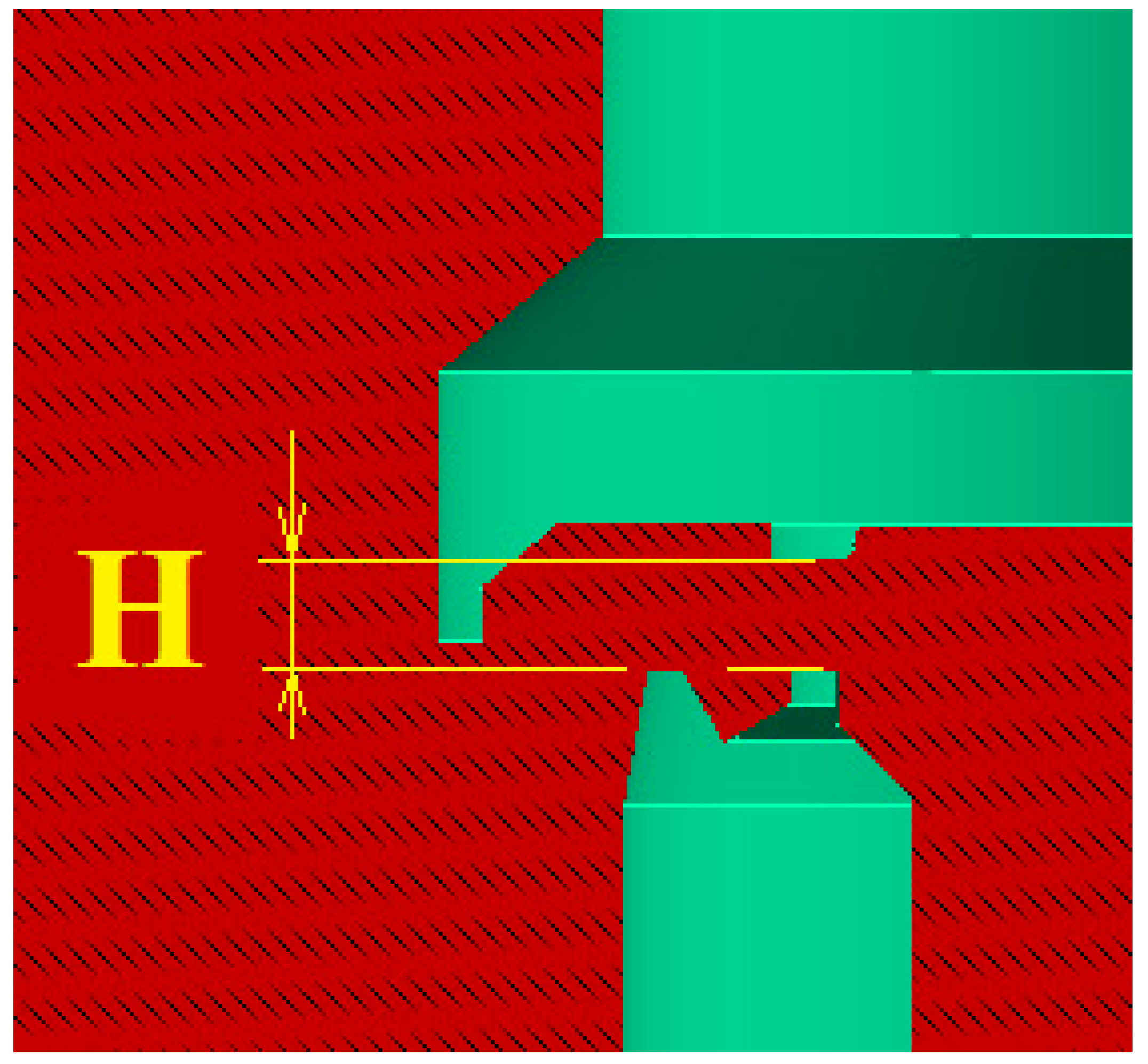
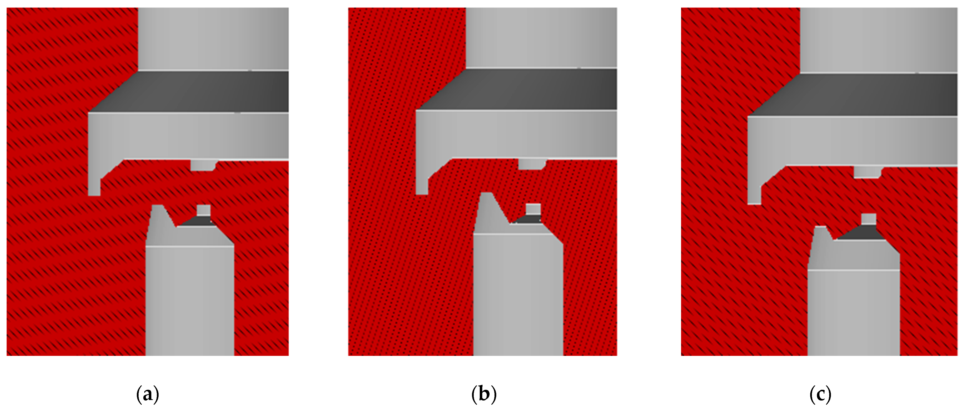
2.1. Characteristics of the Relief Pressure Valve

Figure 1 shows the main components of the pressure valvestudied in this research (commonly used in the oil and gas industry).

Due to the fact that both the sealing surface of the valve and the surface of the seat are covered with hard materials, the valve consists of the valve body and plate, and the seat assembly consists of the seat body and adjusting nozzle. The assembly of these two components, characteristic of discharge valves, is shown in Figure 2.

The geometric model of the fluid part was created in a three-dimensional design program, with small simplifications of its geometry being necessary, with the aim of eliminating possible errors within the CFD simulation. The geometric model of the fluid part is shown in Figure 3.

The technical characteristics of the valve considered in this analysis are presented in

Table 1. Technical characteristics of the valve Dn25/50-Pn40.

Maximum distance seat–valve, [mm]	4
Adjustment pressure, [MPa]	4
Closing pressure, [MPa]	3.4
Discharge pressure, [MPa]	4.4
Pressure	PN40
Material	G20Mn5
Set pressure [MPa]	4
Spring range [MPa]	3.2–4
Maximum temperature [°C]	300
Rated coefficient of discharge	0.7
Applicable medium	Water, oil, gas etc.

. The discharge pressure is the pressure corresponding to the maximum opening of the valve.

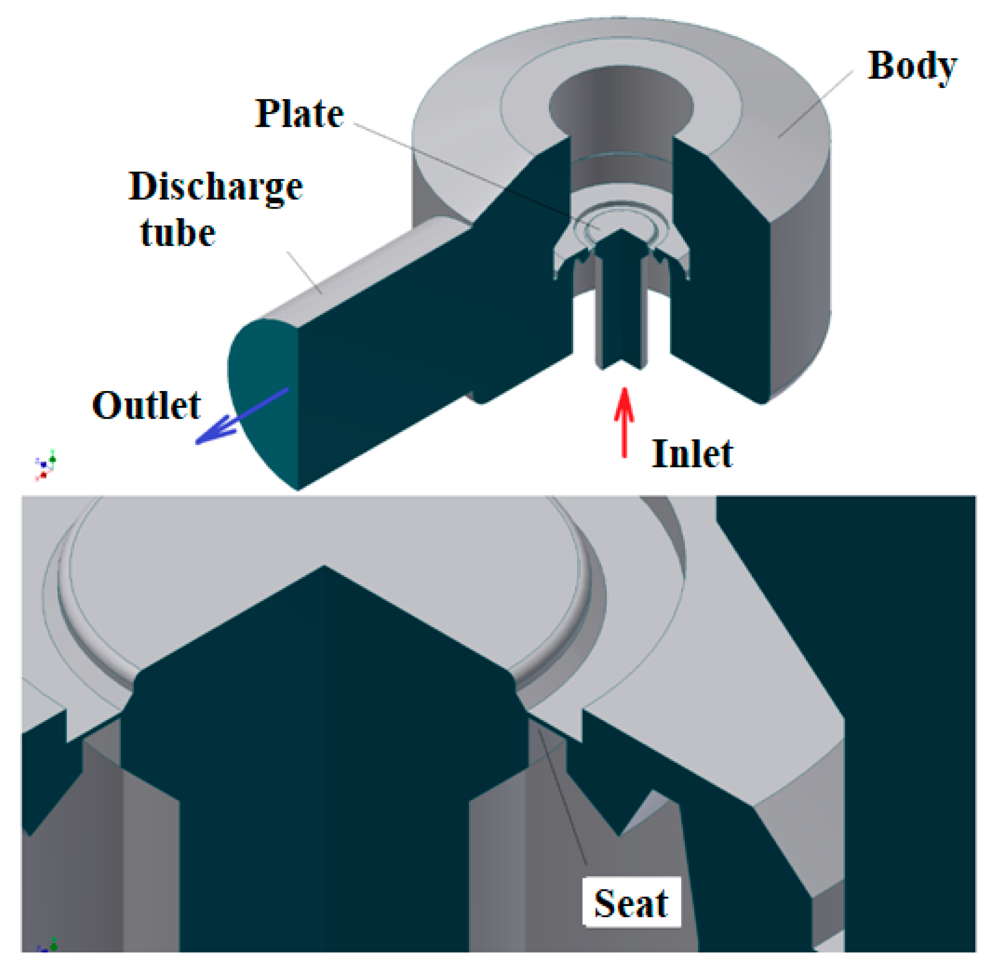
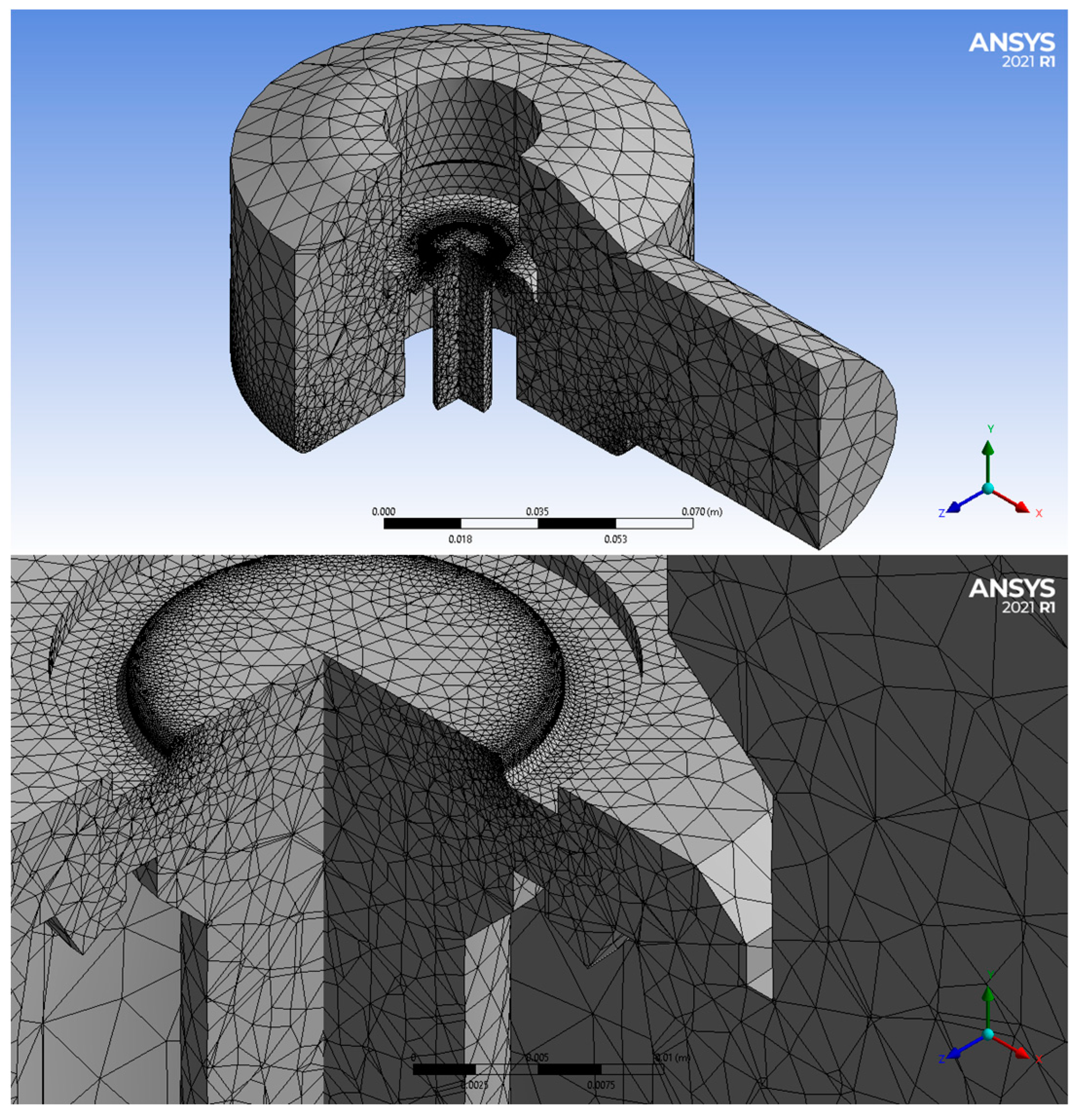
2.2. Calculation Model

2.2.1. The Forces Acting on the Plate

Hydraulic force—is the main force that produces the displacement of the valve plate. This force can act both on the active face of the plate and on its dorsal surface, the analytical expression of this force is given by relation (1).

$$F_h=p·A$$

(1)

where p—is the pressure acting on the plate; A—wetted surface area.

The weight force of the assembly of the movable part of the valve is given by the relationship:

$$F_g=mg$$

(2)

where m—is the total mass of the movable subassemblies in the valve composition; g—gravitational acceleration.

Spring force. During the valve opening process, the force generated by the spring increases due to its compression, given by Hooke’s simple law:

$$F_{el}=-kx=-\left(F_0+k{x}_e\right)=-k\left(x_0+x_e\right)$$

(3)

where F₀ represents the compressive force of the spring when it is compressed by the amount x₀ and x_e—spring compression during valve operation.

Apart from these forces, the friction force, the viscous forces, as well as the damping force also act, but their effect can be neglected compared to the three forces described above [23]. In this case, the mass forces opposing the movement, given by the weight of the rod spring and its fixing elements, represent 9.49 N, so they were neglected. In addition, the rod is guided by a clearance adjustment, which is why the friction force was also neglected.

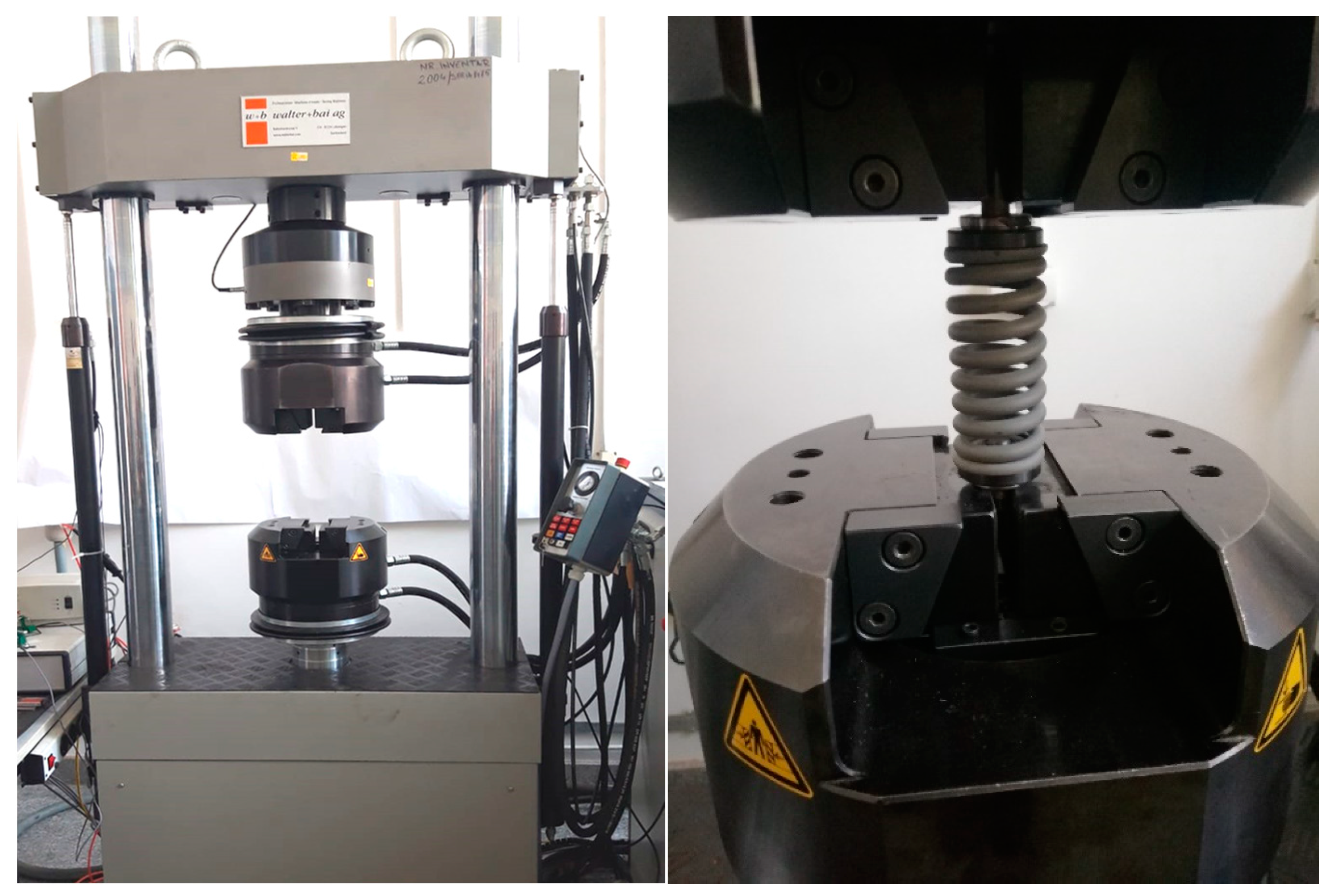
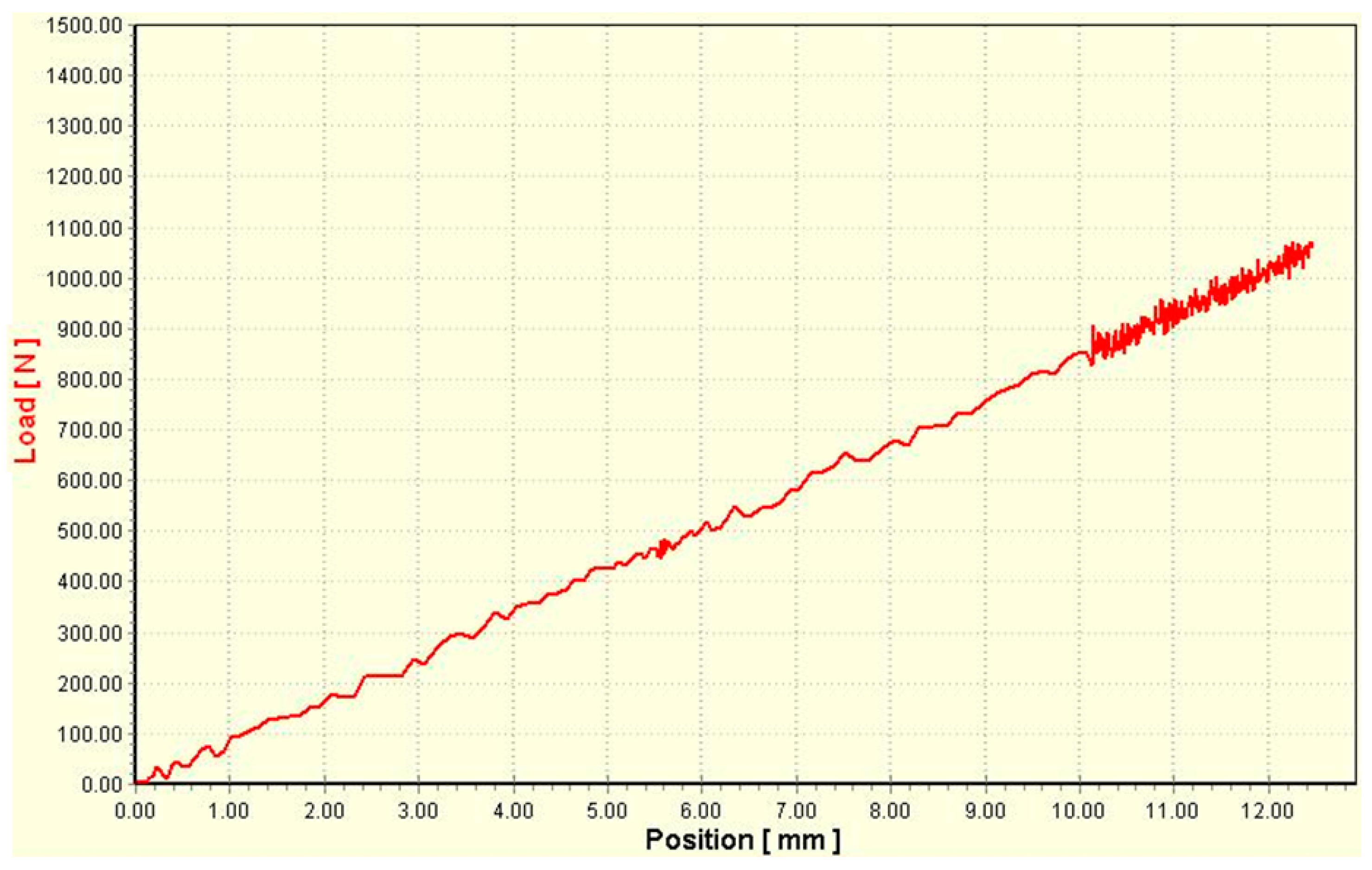
2.2.2. Establishing the Elastic Constant of the Spring

The determination of the elastic constant of the spring (k) from the analyzed valve composition was carried out both analytically and experimentally. The analytical determination of the elastic constant of the spring (stiffness coefficient) was carried out according to relation (4), used in the case of helical springs with a small pitch.

$$k=\frac{G·d^4}{64·n·R^3}$$

(4)

The terms presented in relation (4) are: G, the transverse modulus of elasticity of the spring material; d, diameter of spring wire; n, number of turns; R, mean arc radius. The geometric characteristics of the spring were determined by measurements and are presented in

Table 2. Valve spring dimensions Dn25/50-Pn40.

Wire diameter, d [mm]	7.5
Mean radius, R [mm]	18
The number of turns, n	8.5
Pitch, p [mm]	12.5

.

The determination of the elastic constant of the spring was carried out on the Walter +BAI LF300 tensile testing machine, shown in Figure 4, and the characteristic diagram obtained following the compressive stress of the spring is shown in Figure 5.

The results obtained in the case of determining the elastic constant of the spring, both analytically and experimentally, are presented in

Table 3. The values of the elastic constant of the spring, k.

Analytical determination	85.77 [N/mm]
Experimental determination	83.73 [N/mm]

. The value of the transverse modulus of elasticity was adopted as being: G = 8.5·10⁴ MPa.

It can be seen that the two results are very close, the error between these two determinations being 2.3%. To simplify the calculations, the value of the elastic constant of the spring of 84 N/mm will be adopted.

The CFD analysis of the relief valve aims to simulate the flow of air through the section between the seat and the valve, as well as the influence of its constructive elements on the flow. The simulation was carried out using Ansys-Fluent adopting a tetrahedral mesh obtaining approximately 47,394 nodes and 243,920 elements, as shown in Figure 6. The tetrahedral mesh was adopted after performing a sensitivity analysis making comparison between the results obtained with hexahedral mesh. It was observed that the results were very close, but the computational time was significantly reduced in case of tetrahedral mesh. The same mesh was used in similar works [1,4,23].

To study the behavior of the air flow through the discharge valve, two values of the distance (H) between the seat and the valve were adopted, adistance of 1mm and 4 mm, respectively (corresponding to the maximum opening of the valve), shown in Figure 7. The air pressure at the inlet in the valve is 4.1MPa for H = 1 mm and 4.4 MPa corresponding to the distance H = 4 mm.

To analyze the influence of the adjusting nozzle on the flow through the discharge valve, three positions of it were analyzed: the first—the nozzle is at the same level as the valve seat; second—the nozzle is at the same level as the valve plate; the third—the nozzleis 1.5 mm below the level of the seat face. The latter position was adopted, taking into account certain aspects of the flow. These three situations are shown in Figure 8. To simplify the explanations, the first position of the nozzle was denoted by S0, the second by S1, and the third by S-1.

The flow model adopted in the simulation with ANYSYS Fluent, as well as the values of the adopted parameters are presented in

Table 4. The model adopted in the flow simulation.

The flow model	k-epsilon [1,8,23,24,25,26], Realizable, non-equilibrium wall function [23]
Environment: air/water	Air density: 1.204 kg/m3 Water density: 998.2 kg/m3 Air dynamic viscosity: 1.813·10−5 kg/(m·s) Water dynamic viscosity: 1.003·10−3 kg/(m·s)
Connection conditions	Inlet pressure: (4.1–4.4) MPa Outlet pressure: 0.1 MPa
Type of analysis	Steady, 300 iteration

. It was considered that the pressure at the valve inlet increases proportionally with the distance between the seat and the valve.

Regarding the selection of turbulence models, the impact of different turbulence models on the accuracy of calculations is very important. The performed analysisinvolving the simulation of a pressure relief valve handling water and air as fluids, the choice of the k-epsilon turbulence model aligns well with common practices for such scenarios in CFD, being used in many scientific papers, such as [1,8,23,24,25,26]. Also, this model makes a balance between accuracy and computational efficiency, making it well-suited for engineering analyses [8].The choice to use non-equilibrium wall functions in the simulation, particularly in the context of analyzing air/water flow through a discharge valve, is typically motivated by the flow characteristics near the solid boundaries (such as the valve surface) and the computational efficiency considerations [23].

The concept of wall functions is commonly employed in simulations to model the near-wall behavior of the flow. Near the walls, the turbulence intensity is typically high, and resolving all the turbulent scales in this region would be computationally expensive. Wall functions allow the simulation to model the effects of turbulence close to the wall without explicitly resolving the near-wall region [27,28].The non-equilibrium wall function approach, in the context of the k-epsilon model, refers to a modification of the standard wall functions to account for non-equilibrium effects. In the standard equilibrium wall functions, it is assumed that the flow near the wall reaches a state of equilibrium, meaning that the production of turbulence (turbulent kinetic energy) is balanced by its dissipation. However, in some flows, especially those with strong adverse pressure gradients or complex geometries, the flow near the wall may deviate from equilibrium [28,29].The non-equilibrium wall function approach considers the departure from equilibrium in the near-wall region. It involves additional terms or corrections in the wall functions to account for the non-equilibrium effects on the turbulence quantities (k-epsilon) near the wall. These modifications aim to improve the accuracy of the simulation in capturing the turbulence behavior in challenging flow conditions [29,30,31].

The use of non-equilibrium wall functions in simulations, especially in the context of the k-epsilon turbulence model, can offer several advantages in capturing more realistic turbulent flows, particularly near walls: improved accuracy in complex flows; better representation of near-wall effects; applicability to challenging geometries; enhanced predictions of separated flows; reduced sensitivity to grid resolution; consistency with experimental data; enhanced physical realism.

The fluid flowing through the safety relief valve is assumed to be incompressible in the simulation, as in [7,23]. The statement from [32] emphasizes the practical considerations in fluid dynamics, acknowledging that, in many cases involving liquid service, incompressible flow assumptions are valid. It also acknowledges that for valves designed for gas service, there are situations where the effects of compressibility are minor and incompressible flow models may be applicable.

The convergence was monitored by examining the residual levels and it was decided to adopt 300 iterations, taking into account the computational efficiency and analyzing the residual plots shown in Figure 9, where it can be observed that theresidual showed a consistent trend of reaching a sufficiently low and steady state at 300 iterations.

3. Results and Discussion

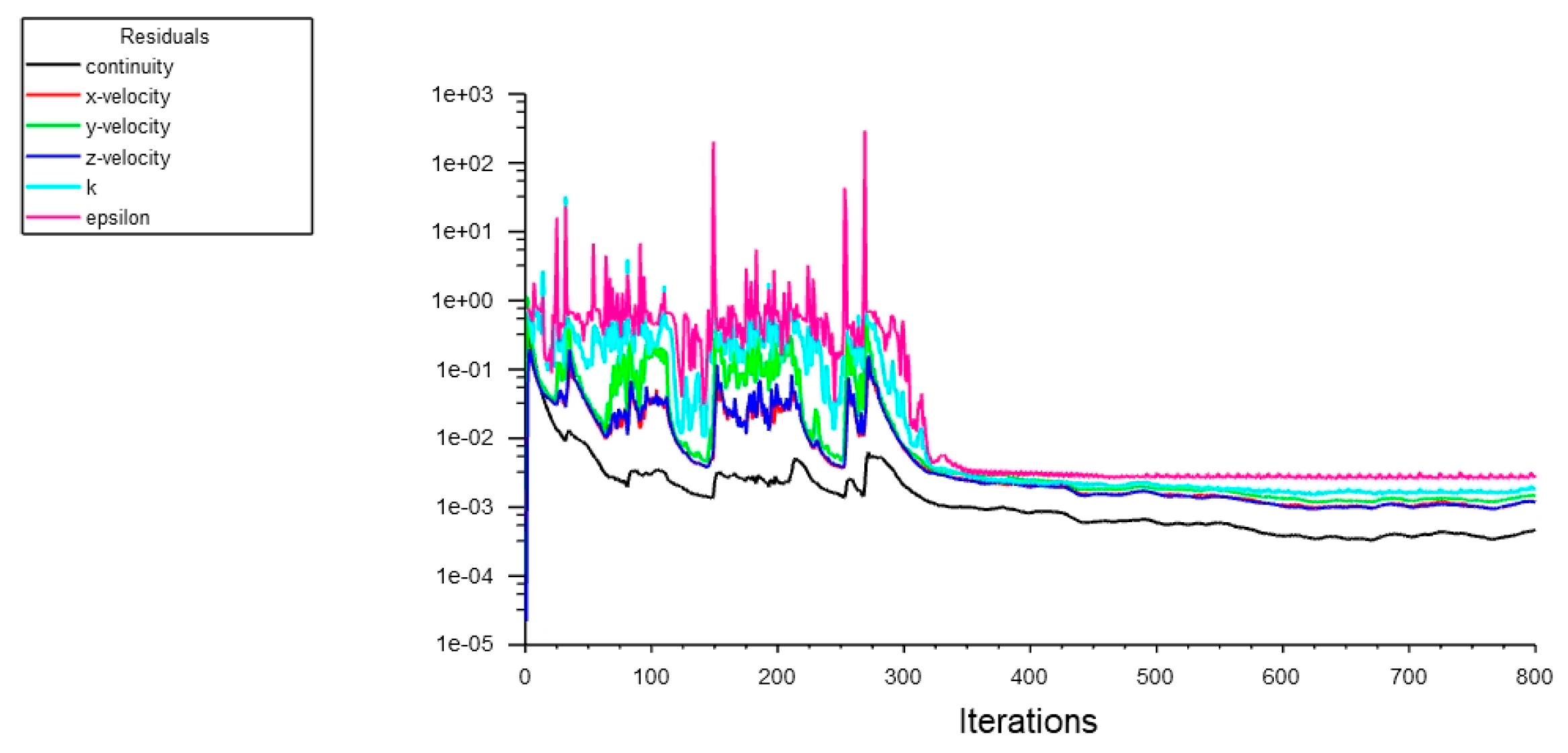
3.1. CFD Analysis

The results obtained regarding the air/water speed for the three positions of the adjustment nozzle according to the distance between the seat and the valve, are presented in

Table 5. Maximum air speed values, [m/s].

Position of Adjusting Nozzle	Seat-to-Valve Distance, H [mm]
	H1		H2		H3		H4
	Air	Water	Air	Water	Air	Water	Air	Water
S0	3080	107	3210	112	3060	108	3160	109
S1	2490	86.7	2940	104	3115	111	3020	105
S-1	2850	99.8	2900	104	3010	105	3010	106

, and its variation graphs are described in Figure 10 and Figure 11.

The first significant observation is the impact of the nozzle position on maximum airspeed. Across all seat-to-valve distances (H), the S0 configuration consistently yielded higher airspeed values compared to S1 and S-1. This suggests that positioning the nozzle at the same level as the seat (S0) promotes higher airflow velocities.

Within each nozzle position category (S0, S1, and S-1), variations in seat-to-valve distance (H) also affect maximum airspeed values. For instance, in the S0 configuration, the highest airspeed of 3210 m/s was achieved at H2, while in the S1 configuration, the maximum airspeed of 2940 m/s occurred at H3. These findings imply that the choice of seat-to-valve distance is a critical factor in determining airflow velocity.

Notably, the S-1 configuration showed relatively consistent airspeed values across different seat-to-valve distances (H), with values ranging from 2850 m/s to 3010 m/s. This suggests that the S-1 configuration may be less sensitive to variations in seat-to-valve distance, providing stability in airflow performance.

In case of water environment, the results from Figure 11 show that the fluidvelocity is significantly influenced by the position of the adjusting nozzle. Notably, when the nozzle is in the S1 position, the fluid velocity is generally lower compared to the S0 and S-1 positions. For instance, the highest fluid velocity observed in the S0 position is 112.0 m/s, whereas the highest fluid velocity in the S1 position is 111.0 m/s. The lowest value of fluid velocity corresponds to the S1/H1 configuration. The seat-to-valve distance also plays a role in affecting the fluid velocity of water through the relief valve. In general, smaller seat-to-valve distances tend to result in lower water velocity’s compared to larger distances. This trend indicates that increasing the distance between the seat and valve allows for increased water flow. Also, to obtain a higher distance between the seat and valve the overpressure was higher as specified in the standard for the safety valve analyzed.

Graphical representations of the results obtained from the CFD simulation regarding pressure, shear stresses and turbulent kinetic energy are depicted in Figure 12, Figure 13, Figure 14, Figure 15, Figure 16 and Figure 17 for the plate and Figure 18, Figure 19, Figure 20, Figure 21, Figure 22 and Figure 23 for the seat.

It is evident that pressure varies considerably across different configurations. In the S0 configuration, the pressure increases with seat-to-valve distance. In the S1 and S-1 configurations, pressure values generally increase until H3, after decrease. This suggests that nozzle position and seat-to-valve distance interact to influence pressure distribution within the valve.

Similar to pressure, shear stress exhibits variations across different combinations of seat-to-valve distances and nozzle positions. For all positions of adjusting nozzle, the maximum shear stress is recorded at H3 distance and is almost equal for all the analyzed configurations. For S1 and S-1 configurations, the minimum values of shear stresses correspond to minimum seat to valve distance (H1), while for S0 configuration it corresponds to the maximum seat to valve distance (H4). The variations in shear stress highlight the complex flow patterns and boundary interactions within the valve.

Turbulent kinetic energy varies significantly, reflecting the turbulent nature of the airflow. The highest value of turbulent kinetic energy is recorded at H2 distance for all the analyzed configurations. Some configurations, such as S-1-H2 and S-1-H4, exhibit notably higher turbulent kinetic energy compared to others. This suggests that specific nozzle-seat combinations may promote more turbulence within the valve.

In the case of water environment, the shear stress is notably affected by nozzle position and seat-to-valve distance. Highest shear stress is observed in the S0 and S1 nozzle positions at 3 mm seat-to-valve distance. Smaller seat-to-valve distances generally result in higher shear stress values. It can be also observed that TKE varies significantly with nozzle position and seat-to-valve distance. Maximum TKE values are found in the S0 and S-1 positions at 2 mm seat-to-valve distance.

Pressure values vary considerably across different configurations. In general, the S0 and S1 configurations exhibit higher pressure values than the S-1 configuration. Additionally, within each configuration, pressure tends to decrease with an increase in seat-to-valve distance. These findings suggest that the choice of nozzle position and seat-to-valve distance significantly affects pressure distribution on the seat.

The shear stress values decrease with seat-to-valve distance, the highest values correspond to S1 configuration, except at H4 distance, where S0 presents the higher shear stress. These variations in shear stress highlight the complex fluid dynamics and boundary interactions occurring on the seat.

Turbulent kinetic energy varies significantly, reflecting the turbulence present in the airflow. In an air environment, generally, the turbulent kinetic energy decreases with seat-to-valve distance until H3. Some configurations, such as S0-H1 and S0-H2, show higher turbulent kinetic energy values compared to others. This suggests that specific nozzle-seat combinations can promote greater turbulence around the seat area.

For example, Figure 24a,b shows the current lines in the case of S0-H1 flow for the air and water environment, respectively. In Figure 25 and Figure 26, the distributions of pressure, shear stress and turbulence kinetic energy for plate and seat, respectively, are presented.

3.2. Statistical Analysis

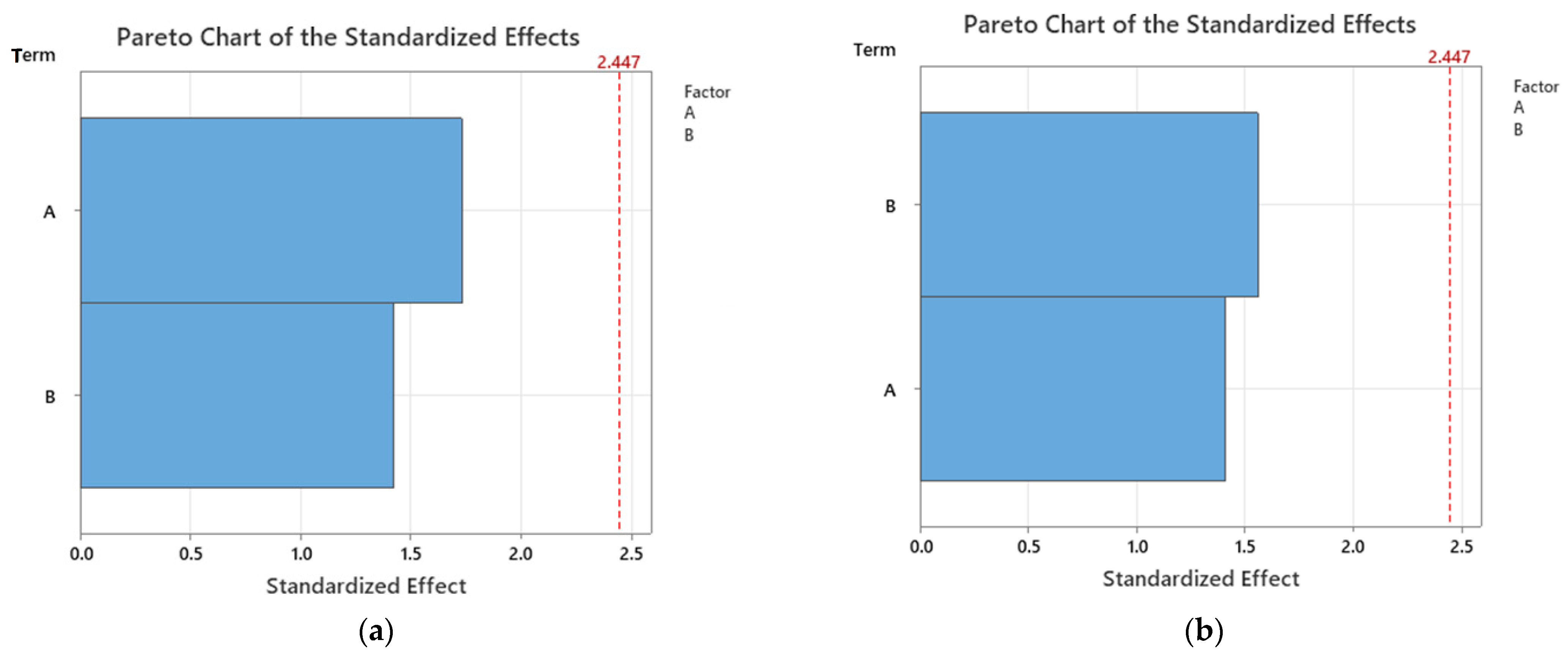
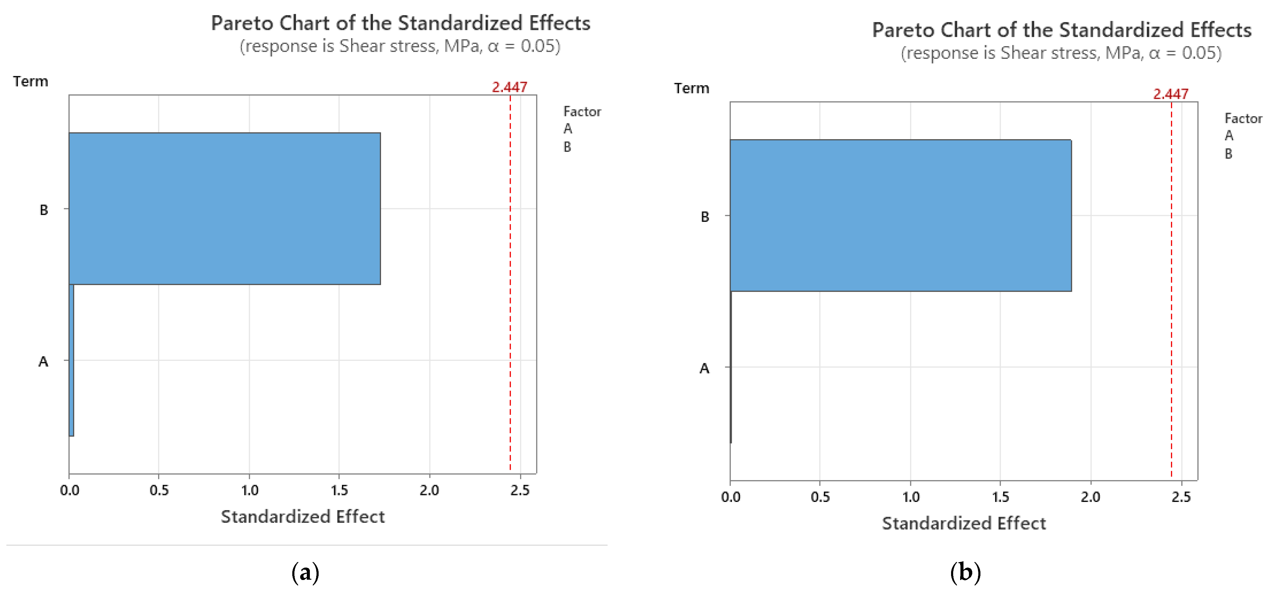
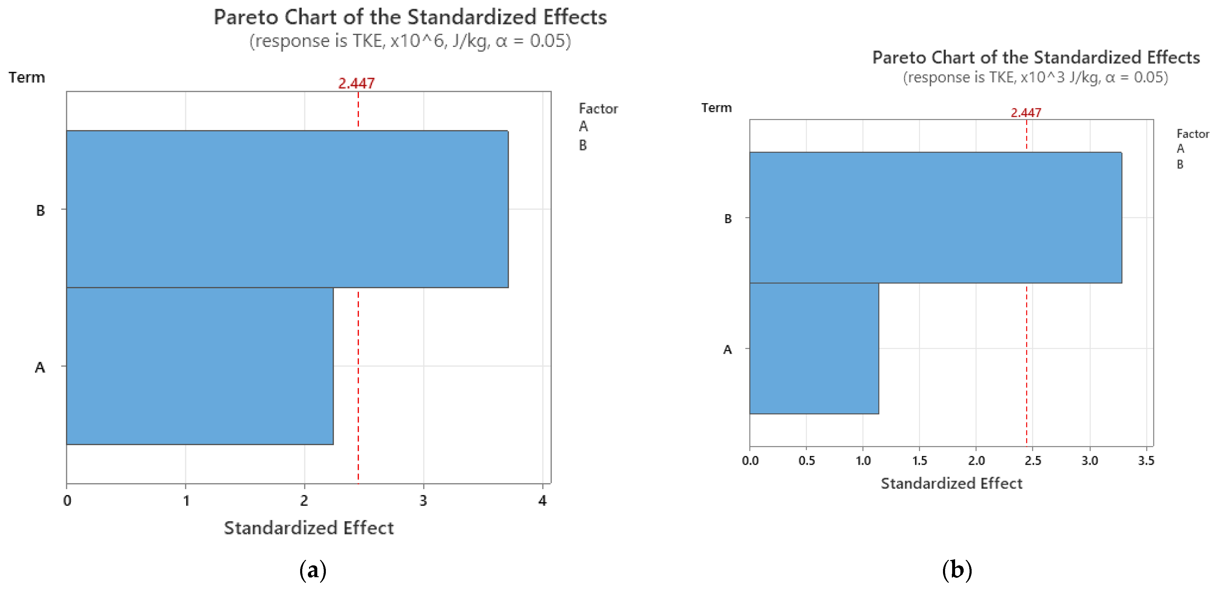
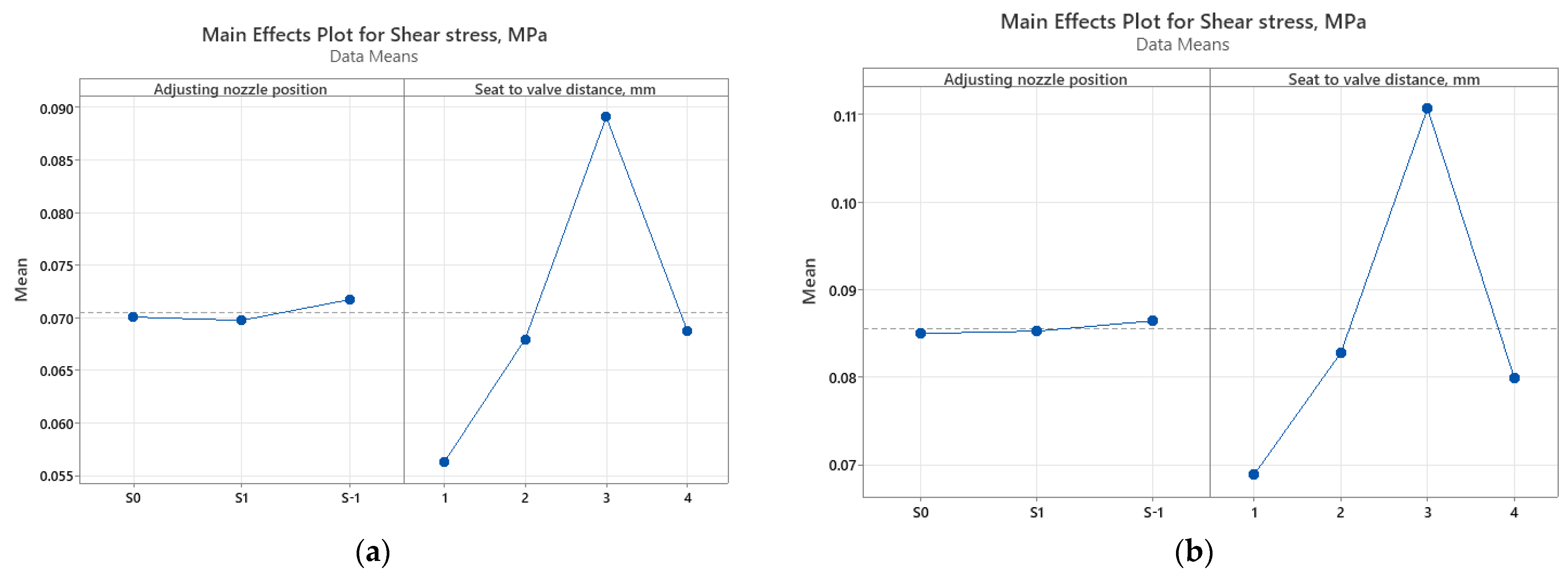
3.2.1. The Relative Significance of Input Parameters

The relative significance of input parameters (A—adjusting nozzle position, B—seat to valve distance), based on their impact, can be effectively illustrated using Pareto charts (Figure 27, Figure 28 and Figure 29). The charts from Figure 27 indicate that, for fluid velocity, adjusting nozzle position emerges as the most critical factor in case of air, whereas in case of water, the seat-to-valve distance is the most significant factor. Regarding the shear stress and turbulent kinetic energy, for both fluids used in the analysis, the factor with the greatest significance is seat to valve distance, as indicated in Figure 28 and Figure 29.

The main effect plot graphs, presented in Figure 30, Figure 31 and Figure 32, reveal a relatively similar evolution of results for both air and water fluids, except for the fluidvelocity parameter when the maximum value corresponds to the S0-H4 configuration for air, while for water, it corresponds to the S0-H3 configuration. As in Figure 28, it can be also highlighted that, in the case of shear stress, adjusting the nozzle position has a very small influence, since the line is almost horizontal (see Figure 31), suggesting that the response mean is the same across all factor levels.

3.2.2. Multi-Response Optimization Using Desirability Function

The optimization analysis was performed to establish the best combination of input parameters (adjusting nozzle position, seat to valve distance) leading to the simultaneously expected evolution of output parameters (fluid velocity, shear stress and turbulent kinetic energy). In the case of fluid velocity, the aim is to maximize it, and the shear stress expected solution is to minimize it, while for turbulent kinetic energy, two situations were investigated since TKE provides a measure of turbulence intensity. Higher TKE levels could be necessary to dissipate excess energy or prevent pressure buildup within the system. In certain applications, such as safety relief valves in high-pressure systems, larger TKE values might indicate that the valve is effectively handling the release of energy and maintaining system safety. In some cases, is preferred to minimize TKE to reduce turbulence within the valve or the downstream flow. Lower TKE values can lead to more stable and controlled flow conditions, which can be advantageous in situations where excessive turbulence could lead to issues like noise, vibration, or erosion of valve components. Smaller TKE values might be desirable when the primary objective is to achieve a more laminar and less turbulent flow.

The optimization was made utilizing the Desirability Function through Minitab 19 software. Desirability analysis assigns values on a scale from zero to one, where a score of one represents the utmost level of suitability.

For the case when the importance is the same for each response, the composite desirability D is calculated with the formula [33,34]:

$$D={\left(d_1\cdot d_2\cdot \dots \cdot d_n\right)}^{1/n}$$

(5)

where n is the number of responses, d_i represents the desirability for each individual response, calculated as [17]:

-

when the goal is to maximize the response desirability:

$$\begin{array}{l}{d}_i=0, if y_i<L_i\\ d_i=\frac{\left(y_i-L_i\right)\cdot r_i}{\left(T_i-L_i\right)}, if L_i\le y_i\le T_i\\ d_i=1, if y_i>T_i\end{array}$$

(6)

-

when the goal is to minimize the response desirability:

$$\begin{array}{l}{d}_i=0, \mathrm{if} y_i>U_i\\ d_i=\frac{\left(U_i-y_i\right)\cdot r_i}{\left(T_i-L_i\right)}, \mathrm{if} T_i\le y_i\le U_i\\ d_i=1, \mathrm{if} y_i<T_i\end{array}$$

(7)

y_i, T_i, L_i, U_i represent the predicted value, target value, lowest and highest value, respectively, of the analyzed response.

Table 6. Composite Desirability and Ranks in case of air environment.

Simulation No	Adjusting Nozzle Position	Seat to Valve Distance, mm	Greater Is Better		Smaller Is Better
			Composite Desirability	Rank	Composite Desirability	Rank
1	S0	1	0.000	10	0.915	1
2	S0	2	0.825	2	0.832	5
3	S0	3	0.000	10	0.716	9
4	S0	4	0.681	7	0.905	2
5	S1	1	0.542	8	0.844	4
6	S1	2	0.810	3	0.790	8
7	S1	3	0.000	10	0.694	11
8	S1	4	0.682	6	0.865	3
9	S-1	1	0.772	4	0.828	7
10	S-1	2	0.839	1	0.704	10
11	S-1	3	0.425	9	0.594	12
12	S-1	4	0.769	5	0.831	6

The highlighted lines correspond to the optimal values (having Rank 1) of input parameters.

and

Table 7. Composite Desirability and Ranks in case of water environment.

Simulation No	Adjusting Nozzle Position	Seat to Valve Distance, mm	Greater Is Better		Smaller Is Better
			Composite Desirability	Rank	Composite Desirability	Rank
1	S0	1	0.364	8	0.728	1
2	S0	2	0.720	1	0.462	7
3	S0	3	0.103	11	0.357	9
4	S0	4	0.550	5	0.703	2
5	S1	1	0.228	9	0.598	4
6	S1	2	0.620	3	0.443	8
7	S1	3	0.000	12	0.312	10
8	S1	4	0.455	6	0.639	3
9	S-1	1	0.436	7	0.577	5
10	S-1	2	0.701	2	0.190	12
11	S-1	3	0.158	10	0.245	11
12	S-1	4	0.582	4	0.572	6

The highlighted lines correspond to the optimal values (having Rank 1) of input parameters.

present the rankings assigned to various configurations of input parameters for the air, respectively, and water environment. The configuration with the highest desirability score in the analysis (highlighted in Table 6 and Table 7) is considered more suitable according to the criteria and objectives defined for the analysis.

The plots for optimization (Figure 33 and Figure 34) visually depict the impact of individual factors (presented in columns) on the responses or composite desirability (displayed in rows). In these graphs, the red lines indicate the existing factor settings, and the red numbers at the top of each column represent the current levels of these factors. The horizontal blue lines, along with their associated numbers, show the responses linked to the current factor levels.

The optimization process indicated the following combination of input parameters to achieve the expected outcomes:

✓

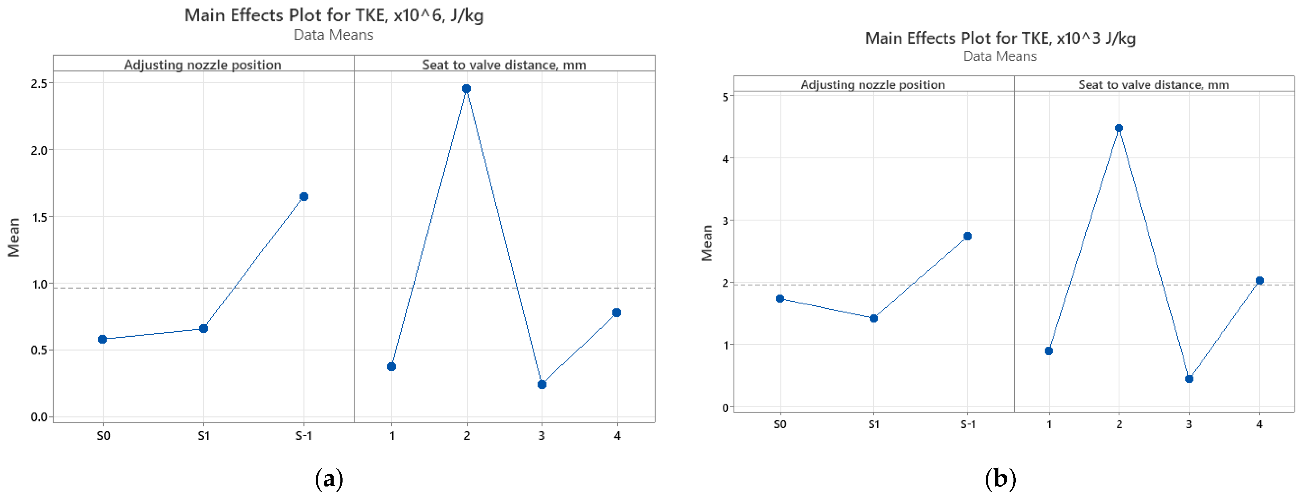
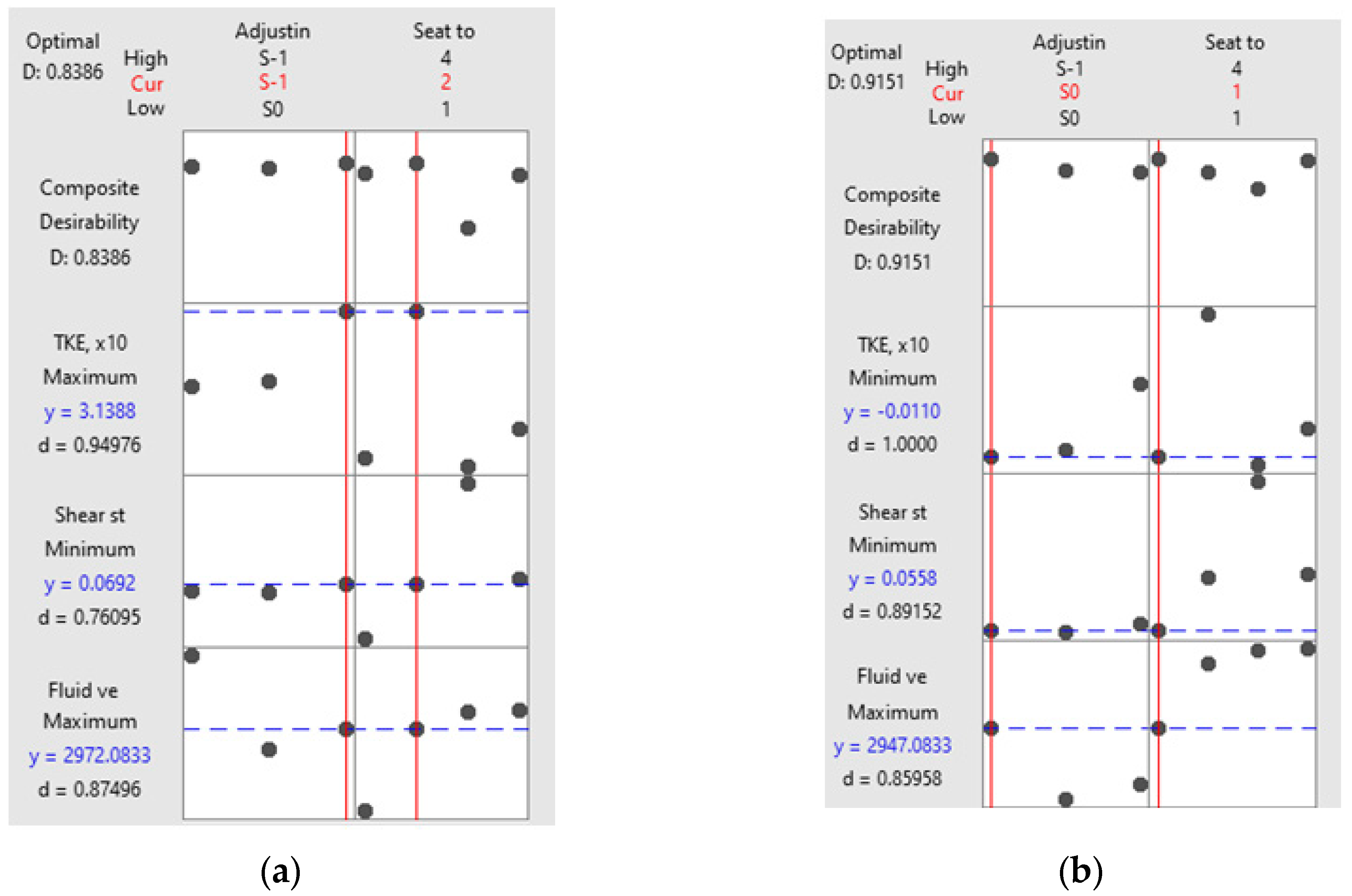
for the air environment: S-1/H2 for “greater is better” option of turbulent kinetic energy and S0/H1 for “smaller is better” option of turbulent kinetic energy;

✓

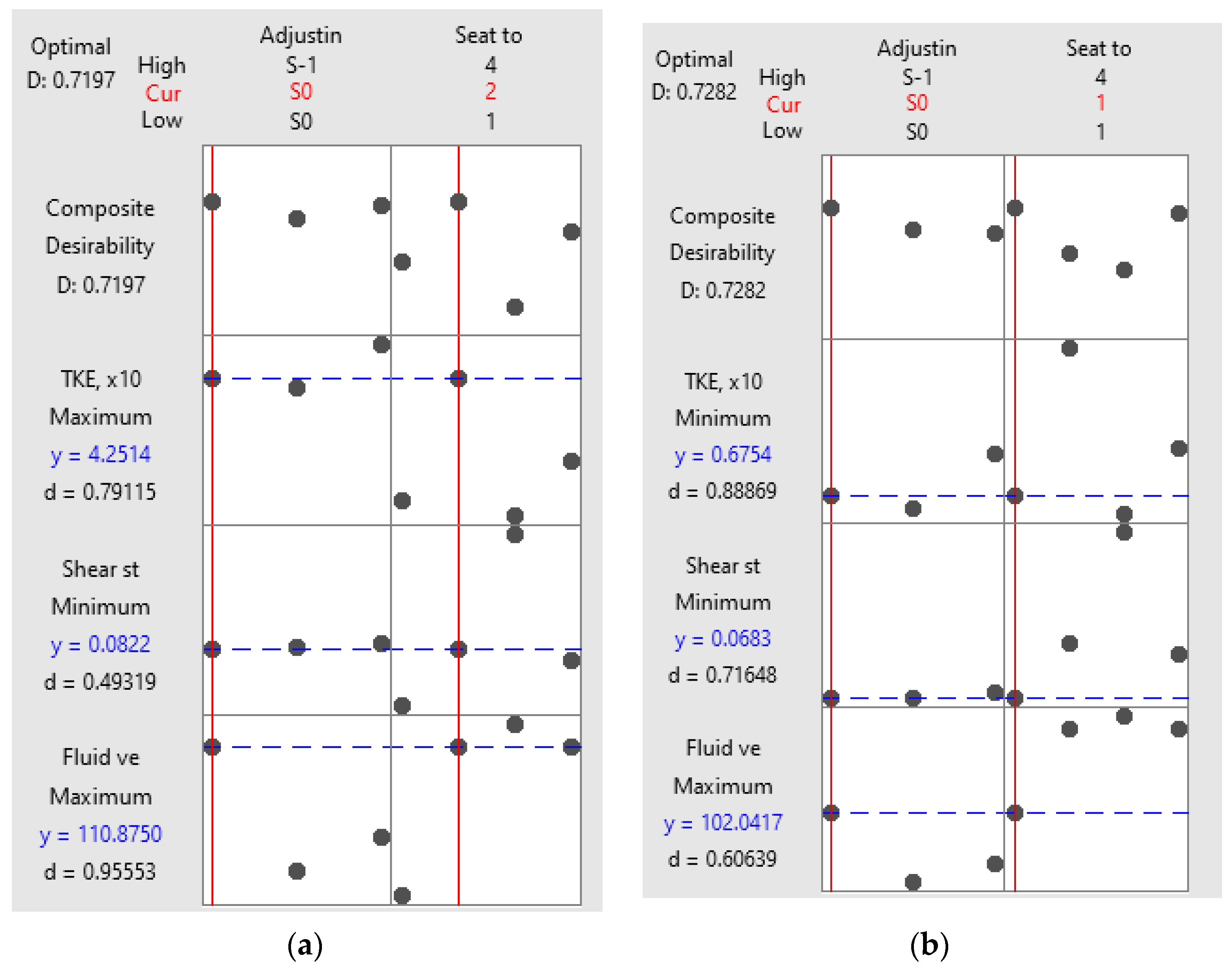
for the water environment: S0/H2 for “greater is better” option of turbulent kinetic energy and S0/H1 for “smaller is better” option of turbulent kinetic energy.

3.3. Synthesis of Results

✓

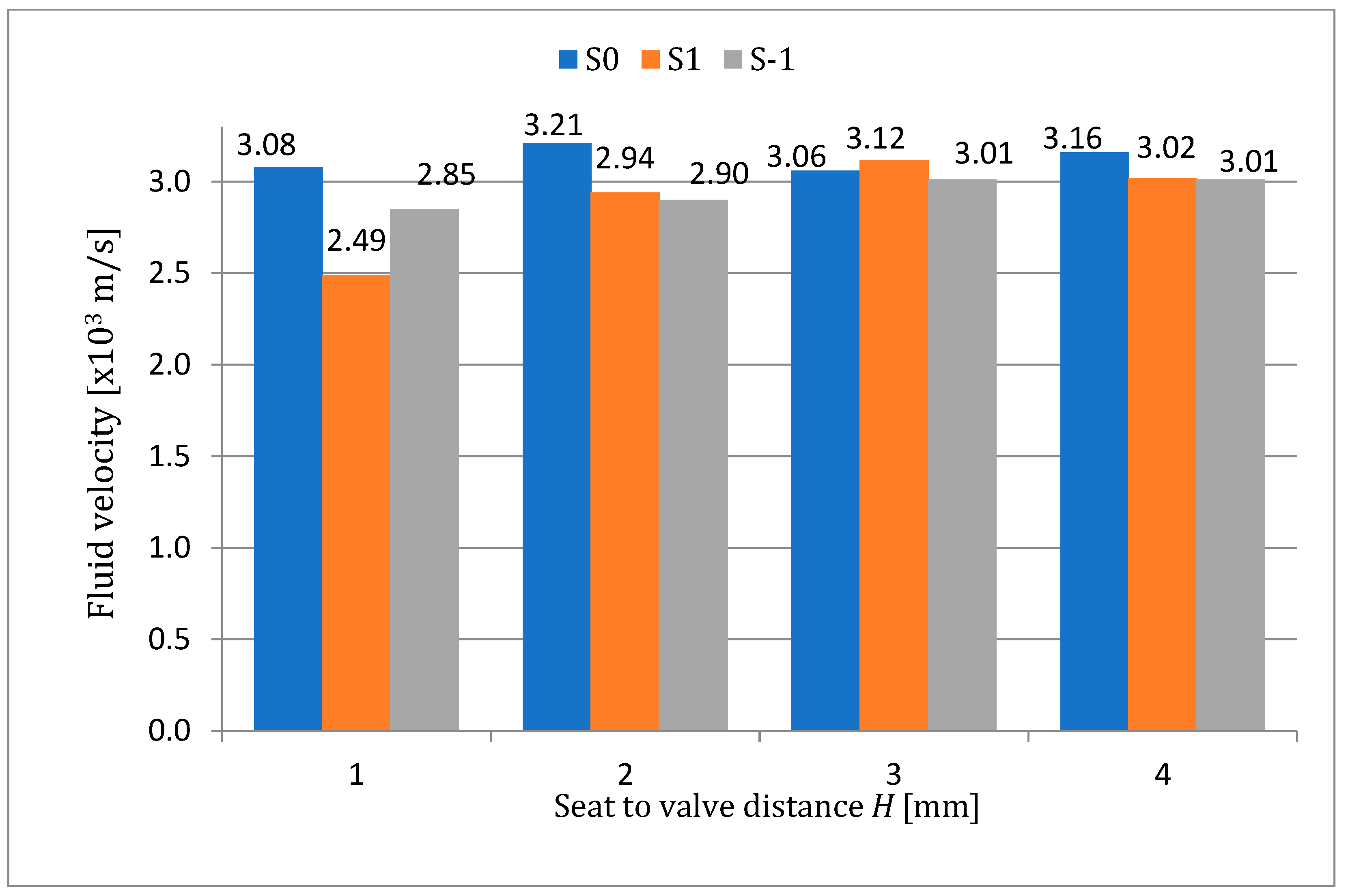
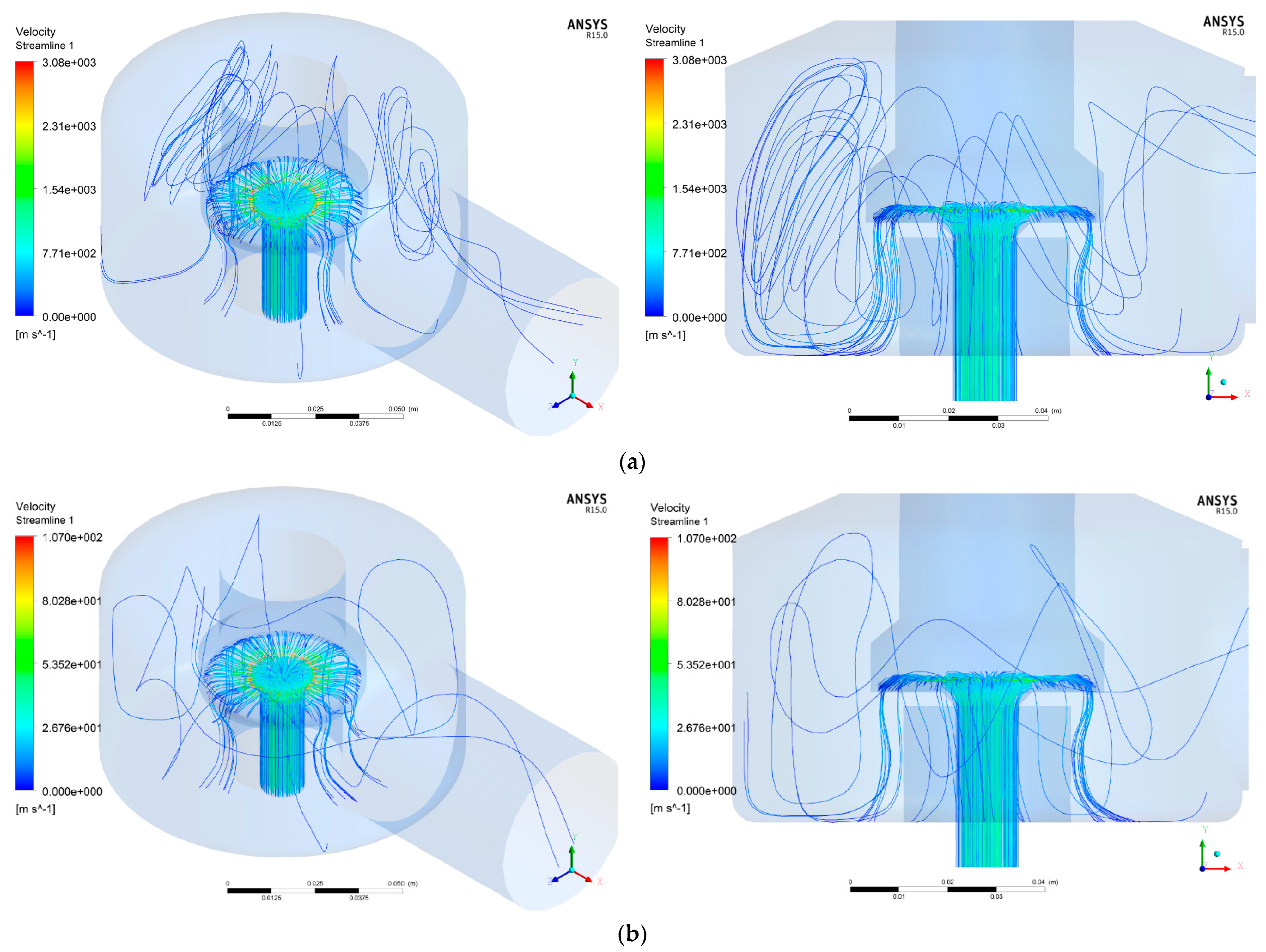
In most of the analyzed cases, the maximum airspeed was obtained in the space between the seat and the valve, this having the value of 3210 m/s for the S0-H2 case. For cases where the adjusting nozzle is at or below the seat, the variation in air velocity is relatively small. The calculated velocity difference between the extreme values is 150m/s for position S0 and approximately 160m/s for S-1.

✓

For nozzle position S1, the air velocity varies significantly compared to the other two, with the minimum value being 2490 m/s for H1. At high fluidvelocity, the vortices created inside the valve body are much more pronounced, but the streamlines respect its geometric configuration.

✓

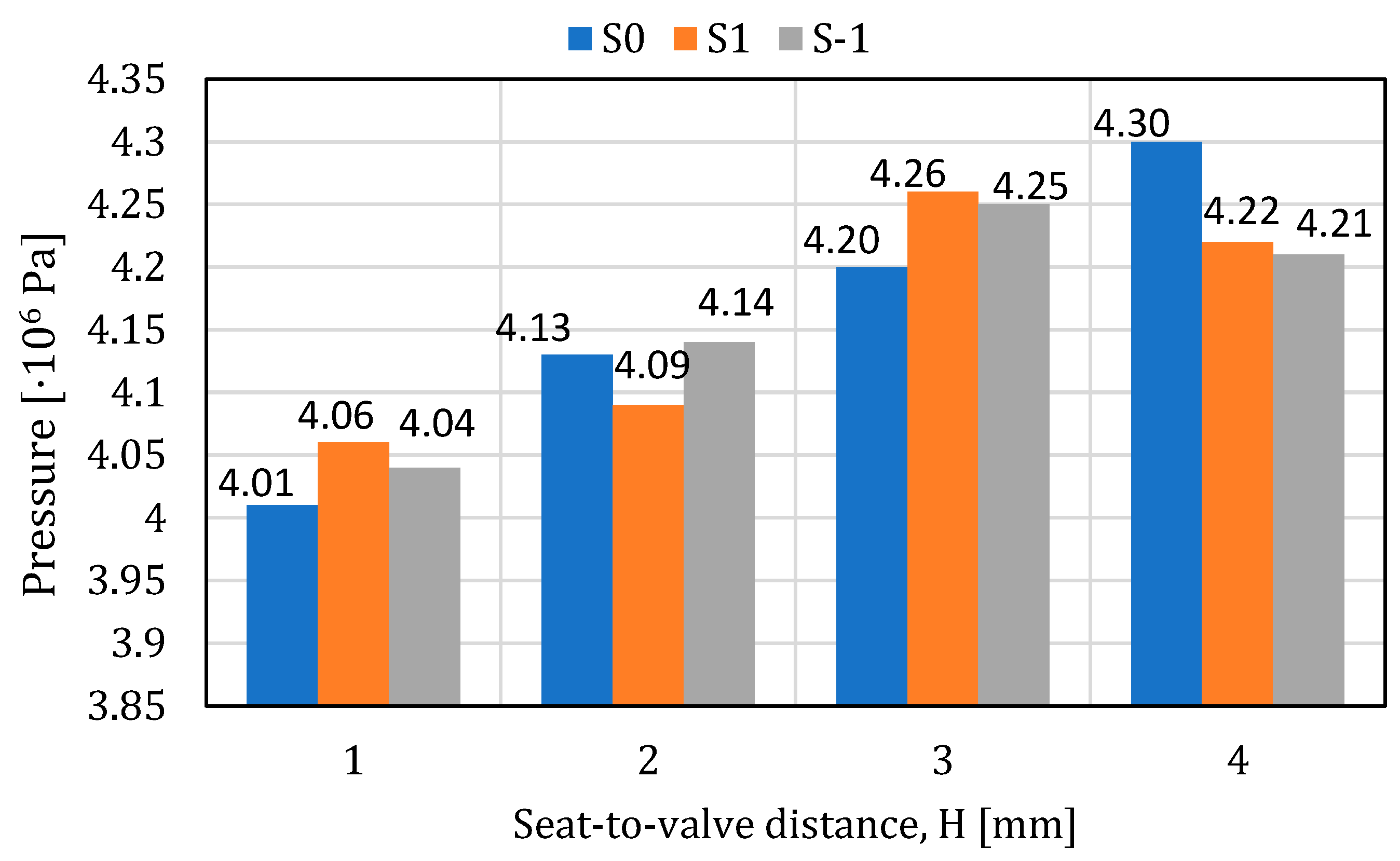
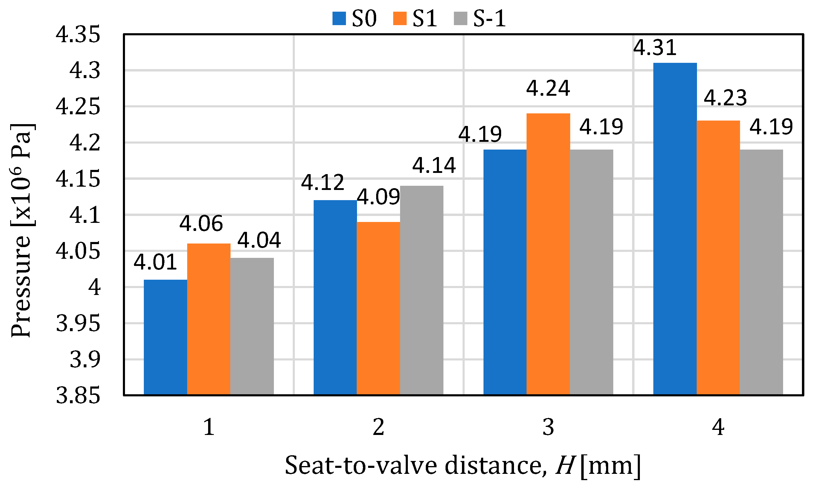
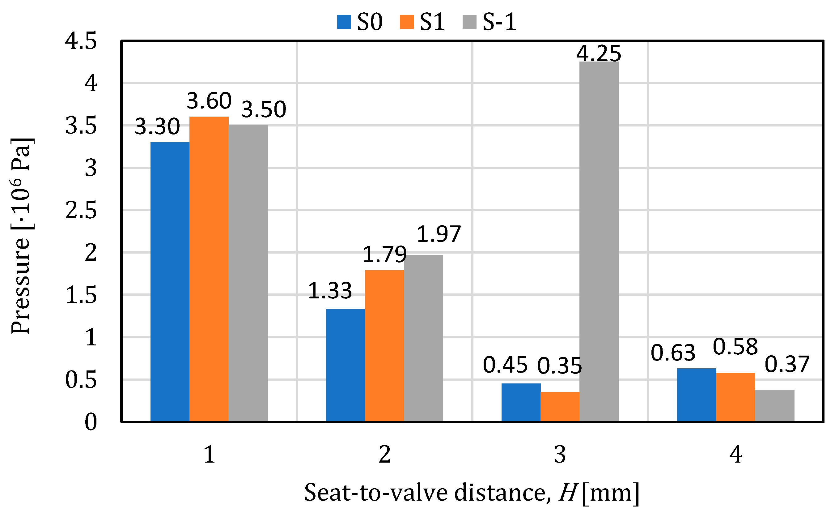
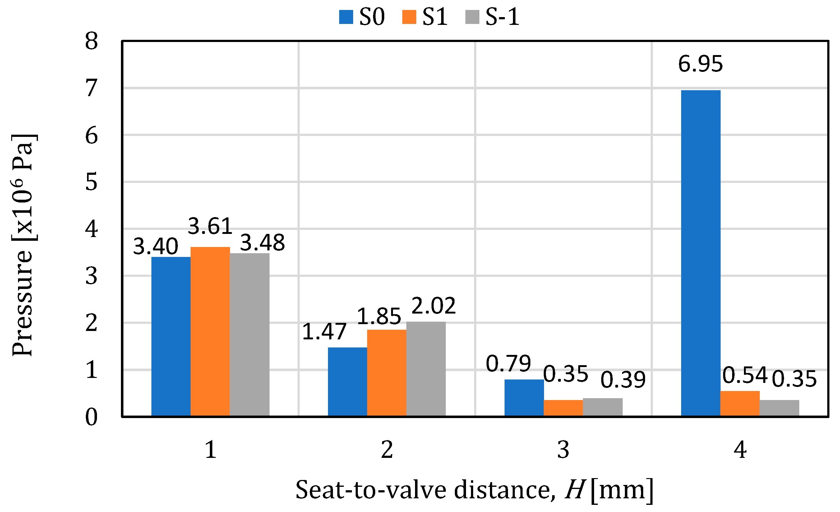
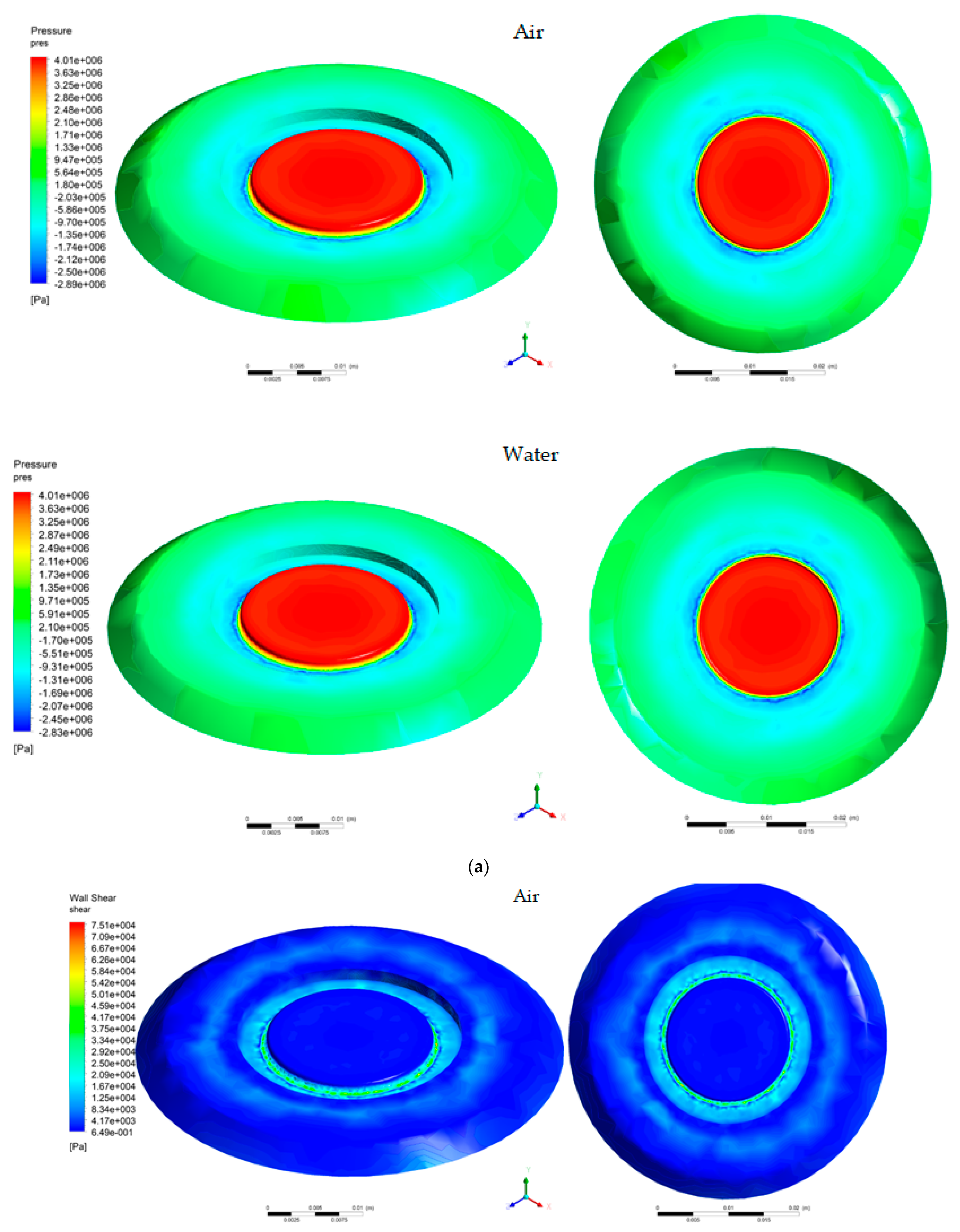
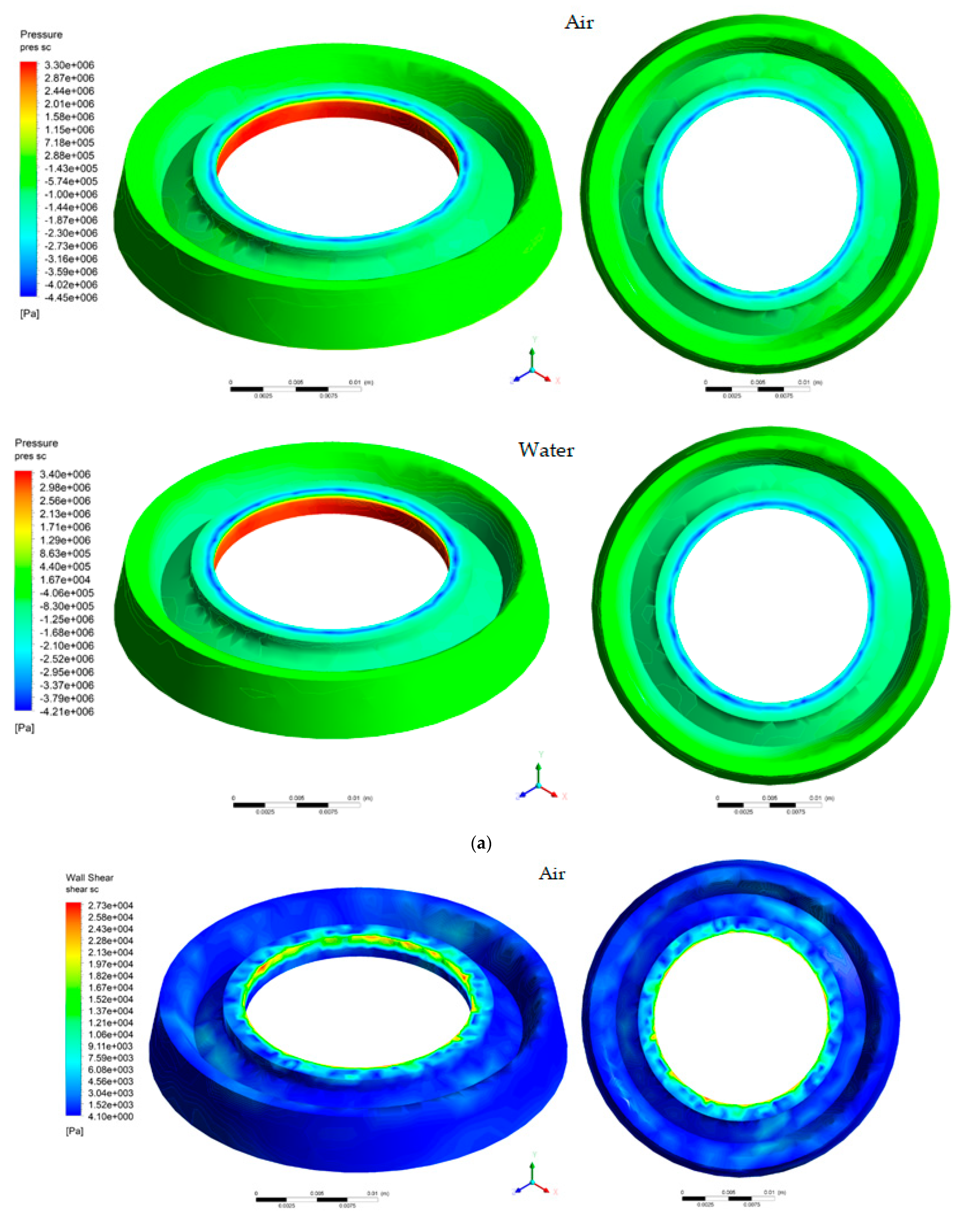
In all analyzed cases, the extreme pressure values were obtained on the circular surface in the center of the plate. The highest value of the pressure is 4.3 MPa (air) and 4.31 MPa (water), being evenly distributed on the plate surface. In the case of the seat, the pressure drops with valve lift for all three positions of the adjusting nozzle except S-1-H3 (in air environment) and S0-H4 (in water environment).

✓

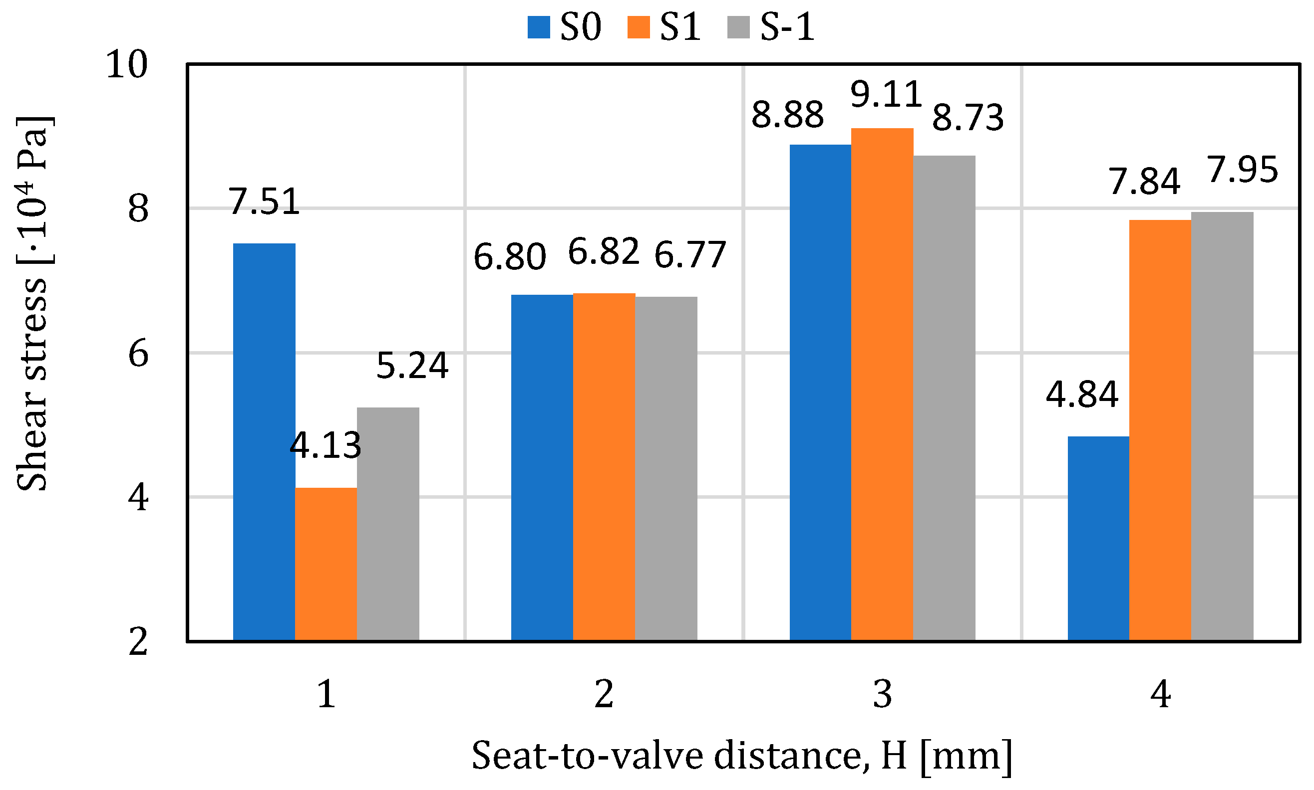
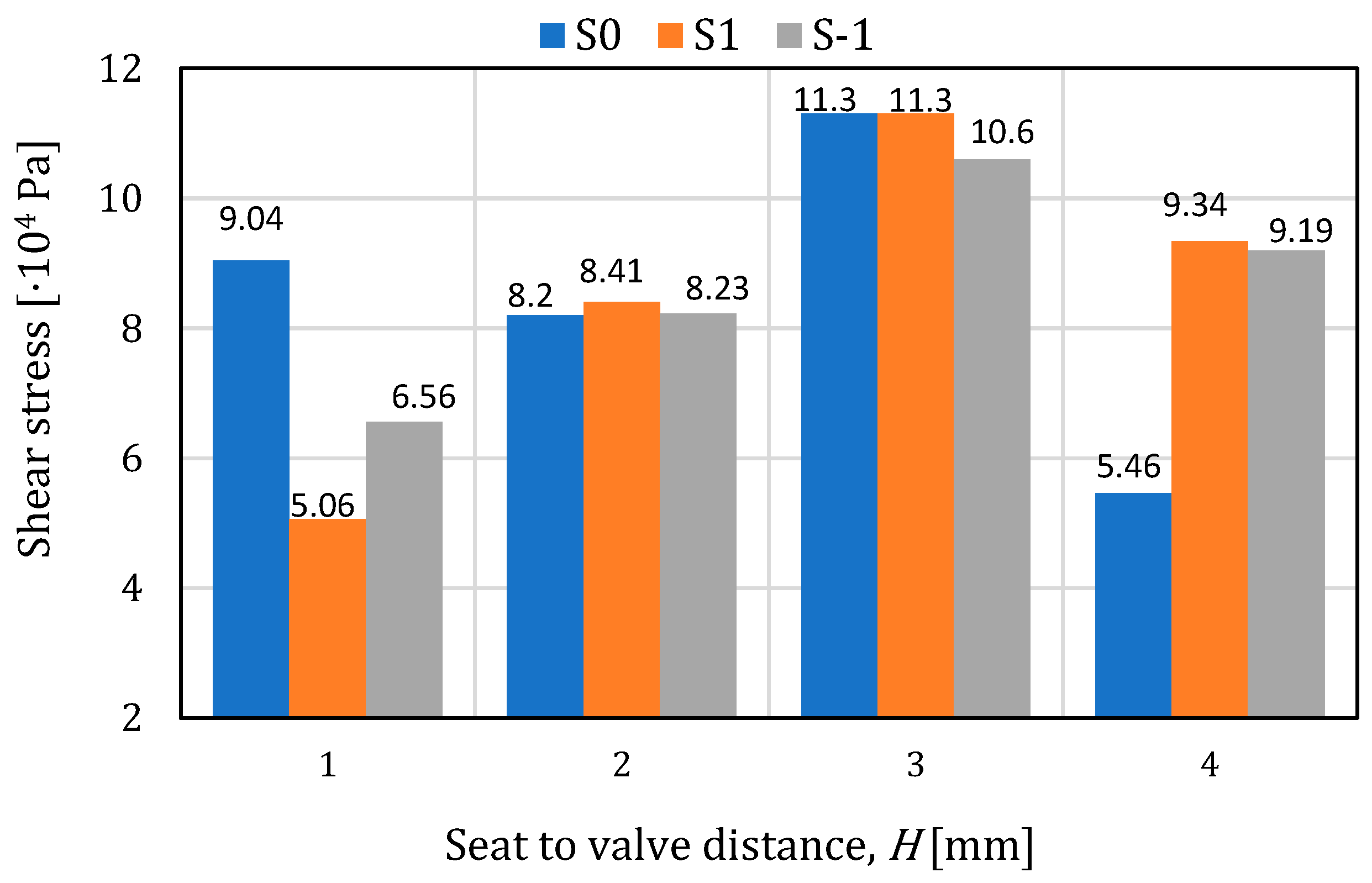
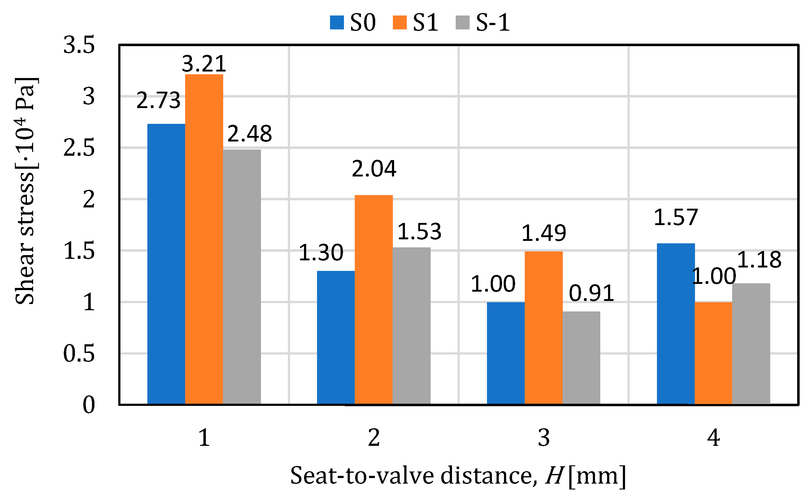
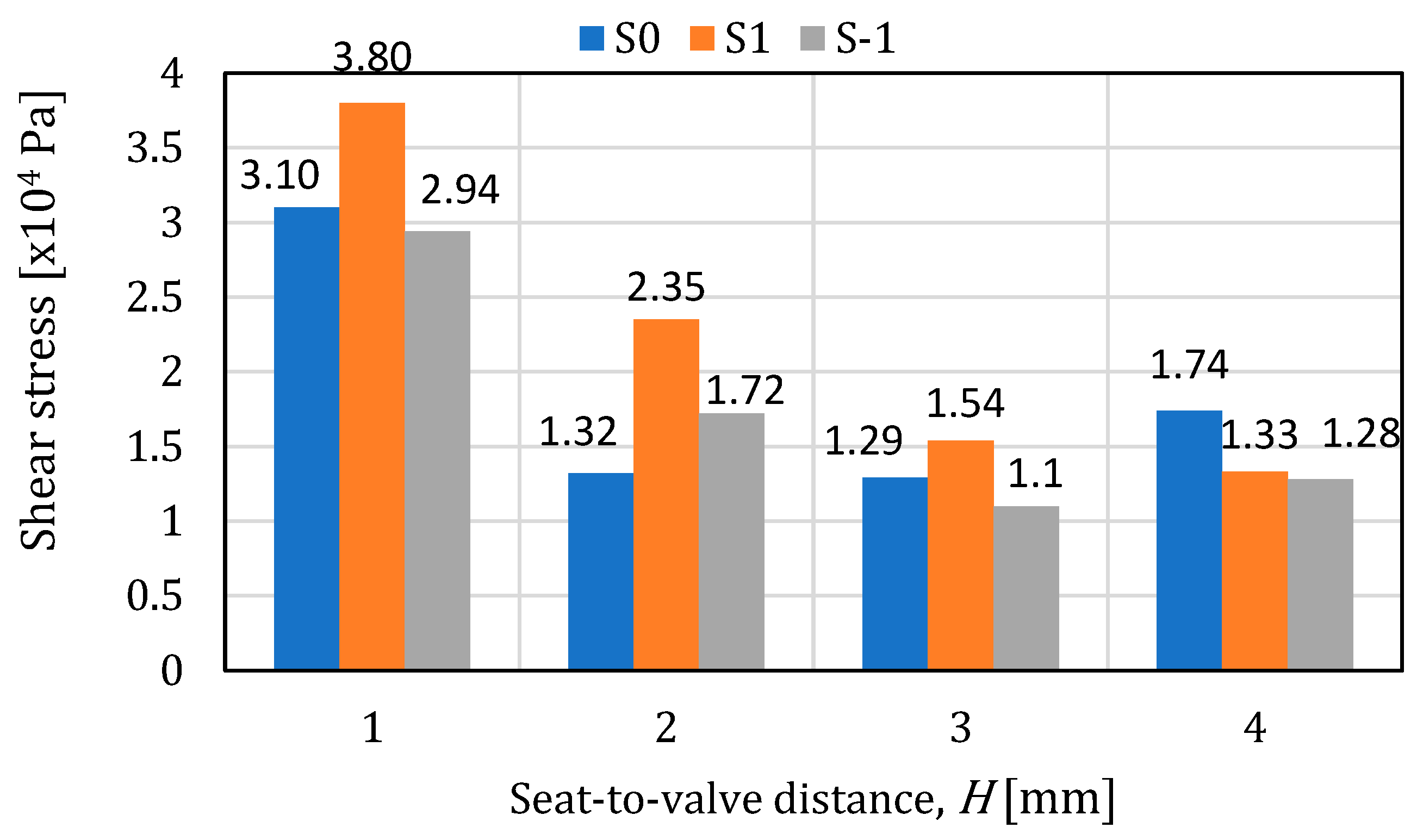
The maximum values of the tangential stresses on the plate appear in most cases on the surface of the 0.4mm chamfer, and in the case of the seat, they vary randomly on its surface. The maximum value of the tangential stresses on the plate is 0.0911 MPa (air) and 0.113 MPa (water), and in the case of the seat, the maximum values were obtained at H1, having a decreasing variation depending on the seat–valve distance.

✓

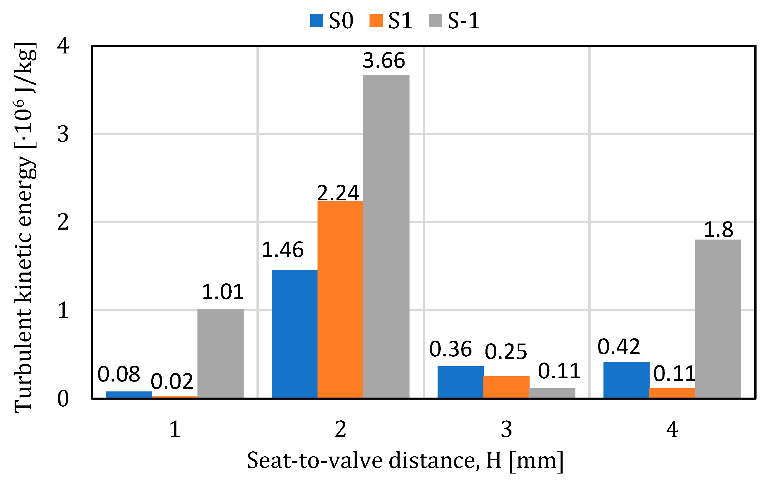
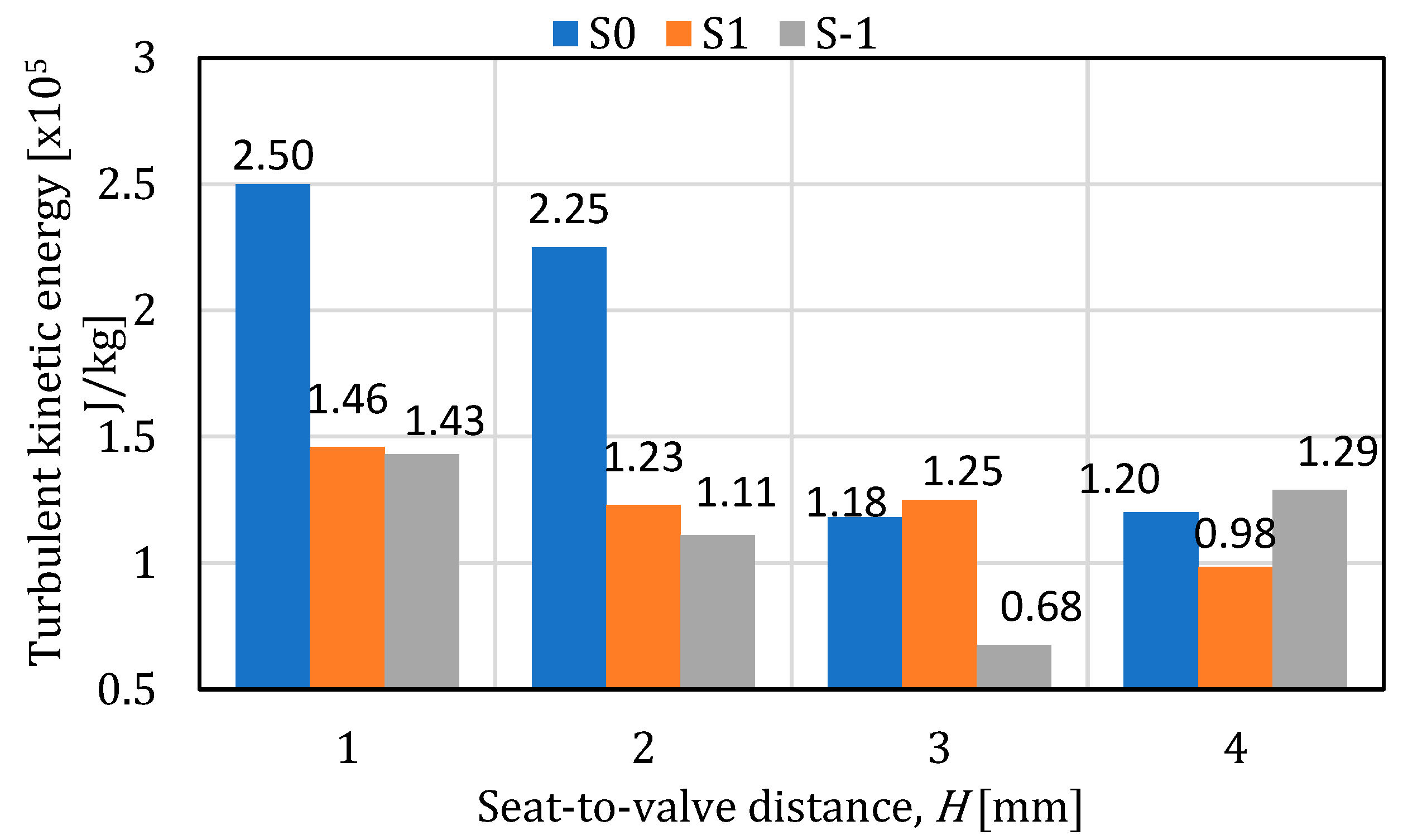
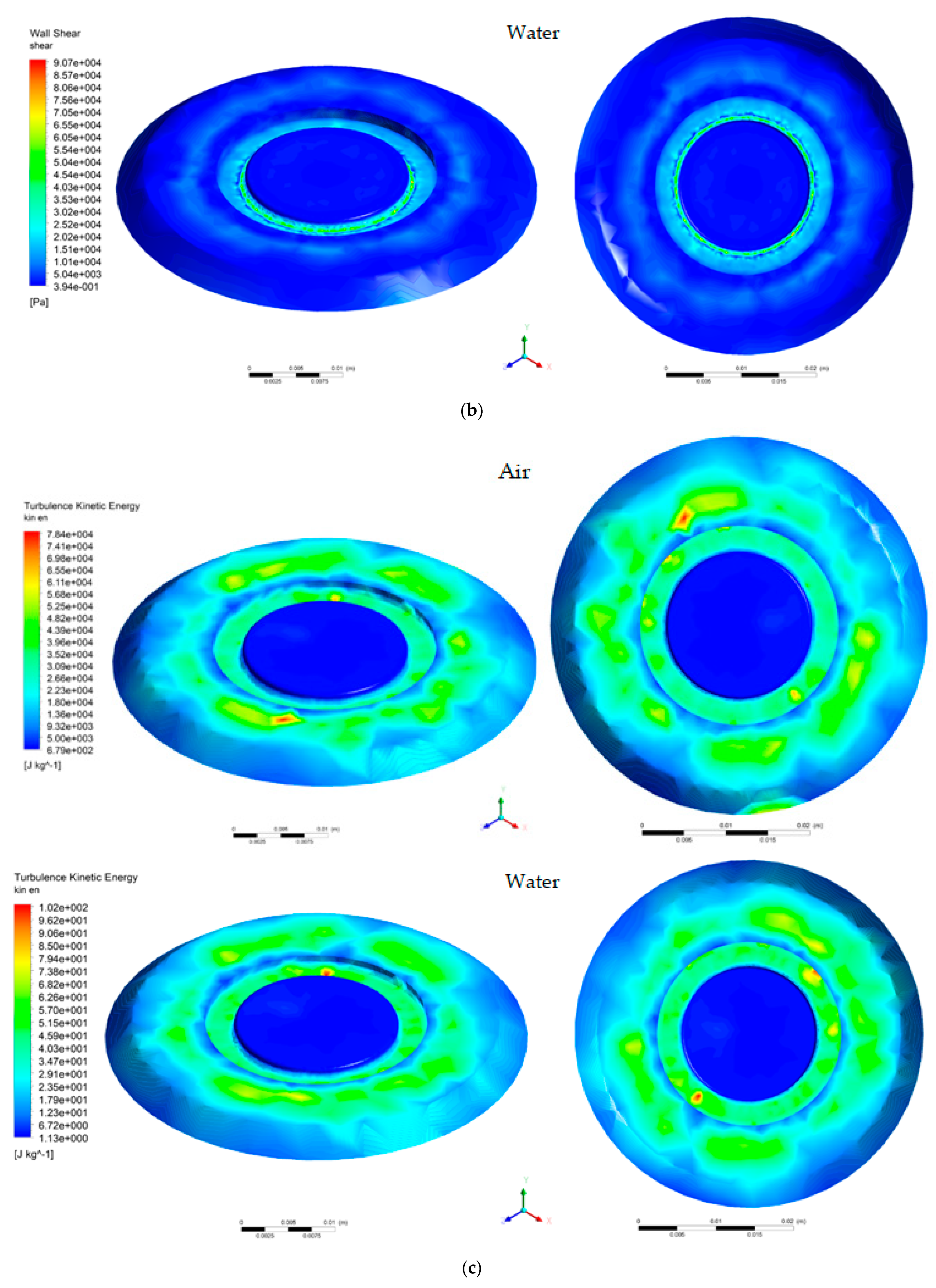
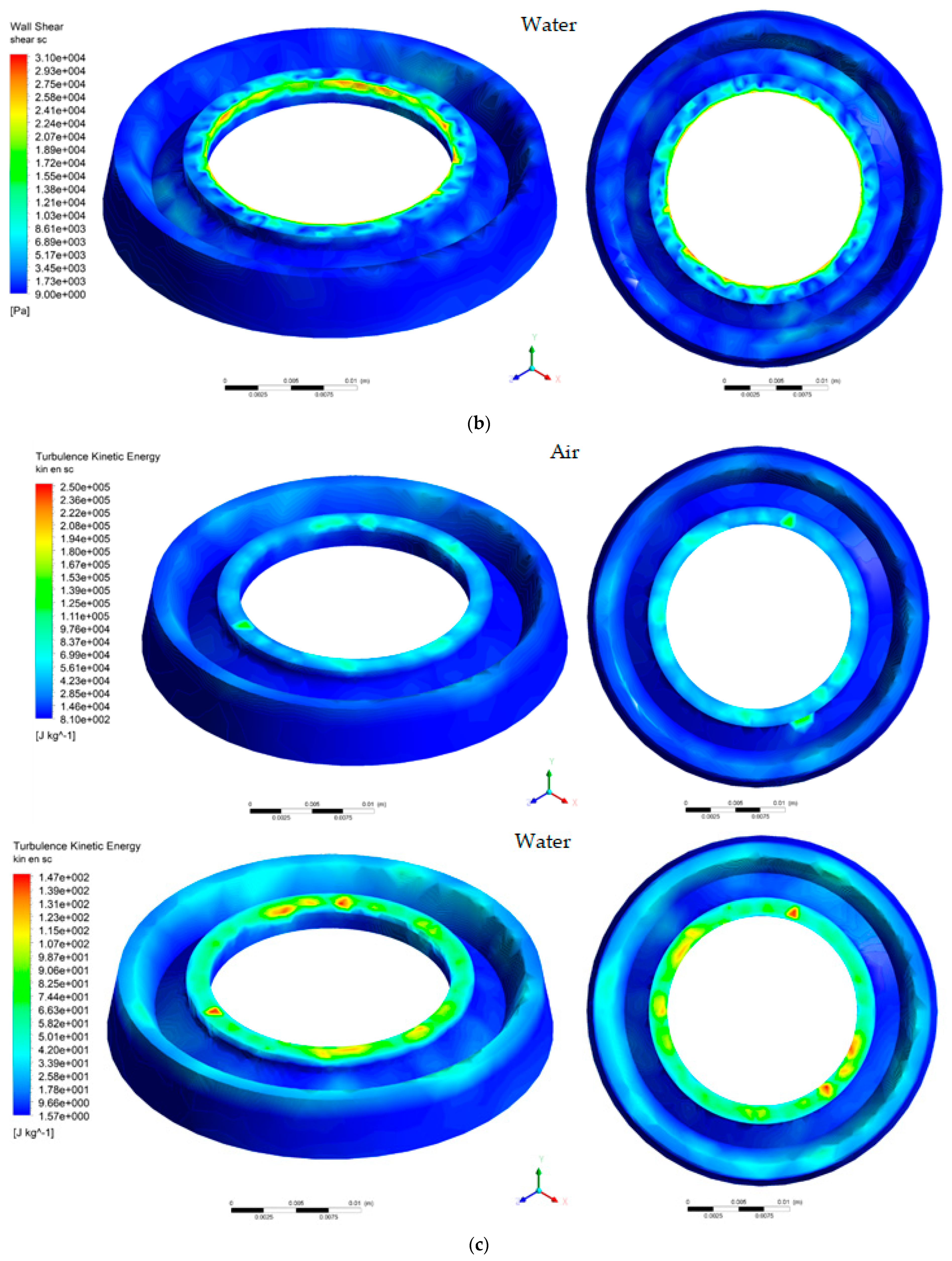
In air environment, the turbulent kinetic energy has a random distribution over the surface of both the plate and the seat. In the case of the plate, the maximum value is 3660kJ/kg and was obtained in the S-1-H2 configuration. In the case of the seat, the turbulent kinetic energy has a relatively uniform variation for positions S1 and S-1, the highest value was obtained in the case of S0-H1, being 78.4kJ/kg.

✓

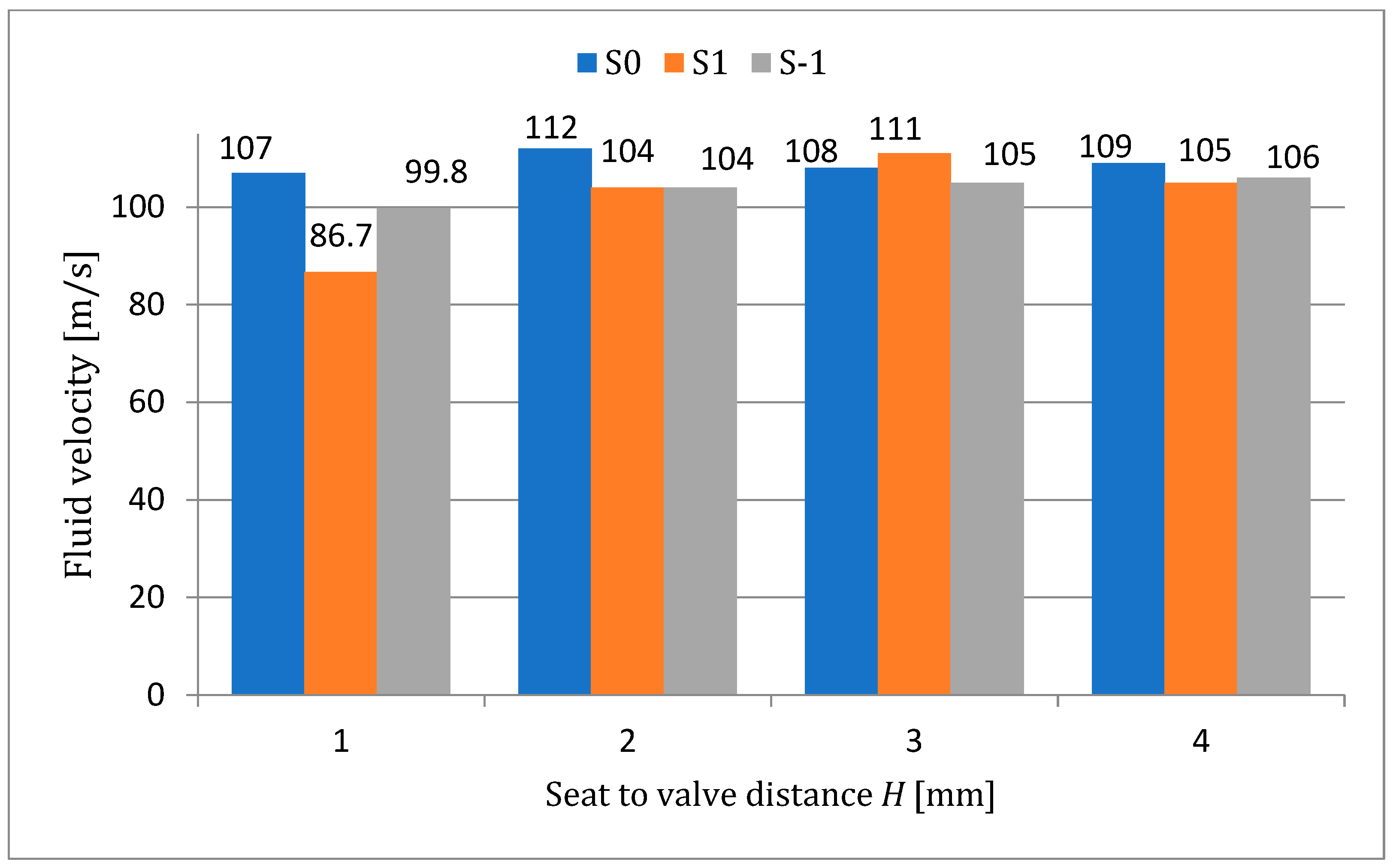
In most of the analyzed cases, the maximum water speed was obtained in the space between the seat and the valve, this having the value of 112 m/s for the S0-H2 case. For cases where the adjusting nozzle is at or below the seat, the variation in water velocity is relatively small. The calculated difference between the extreme values is 5 m/s for the nozzle position S0 and about 6 m/s for S-1.

✓

In the case of nozzle position S1, the watervelocity varies significantly compared to the other two, with the minimum value being 87 m/s for H1. At high fluid velocity, the turbulence created inside the valve body is much more pronounced, but the streamlines follow its configuration.

✓

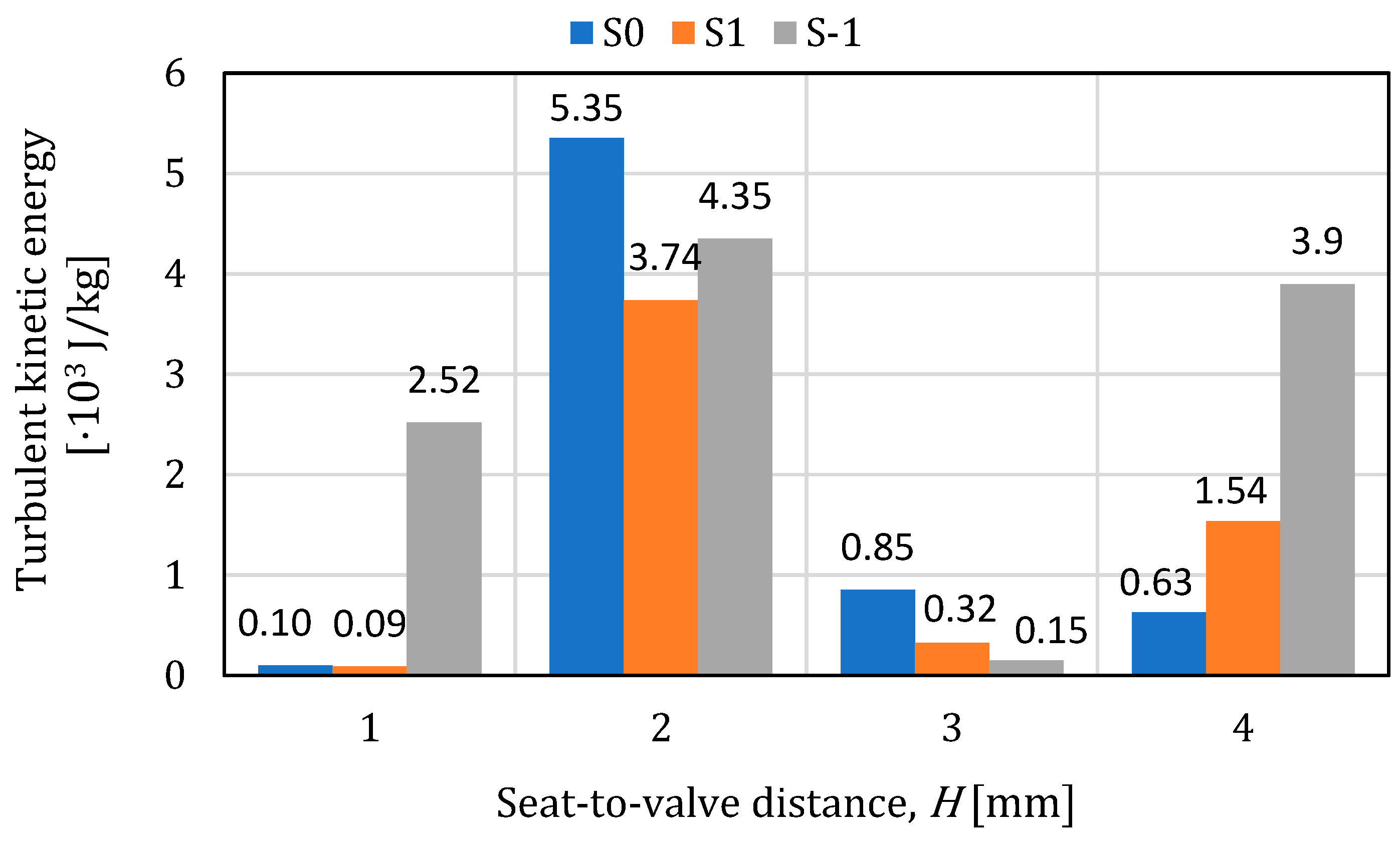
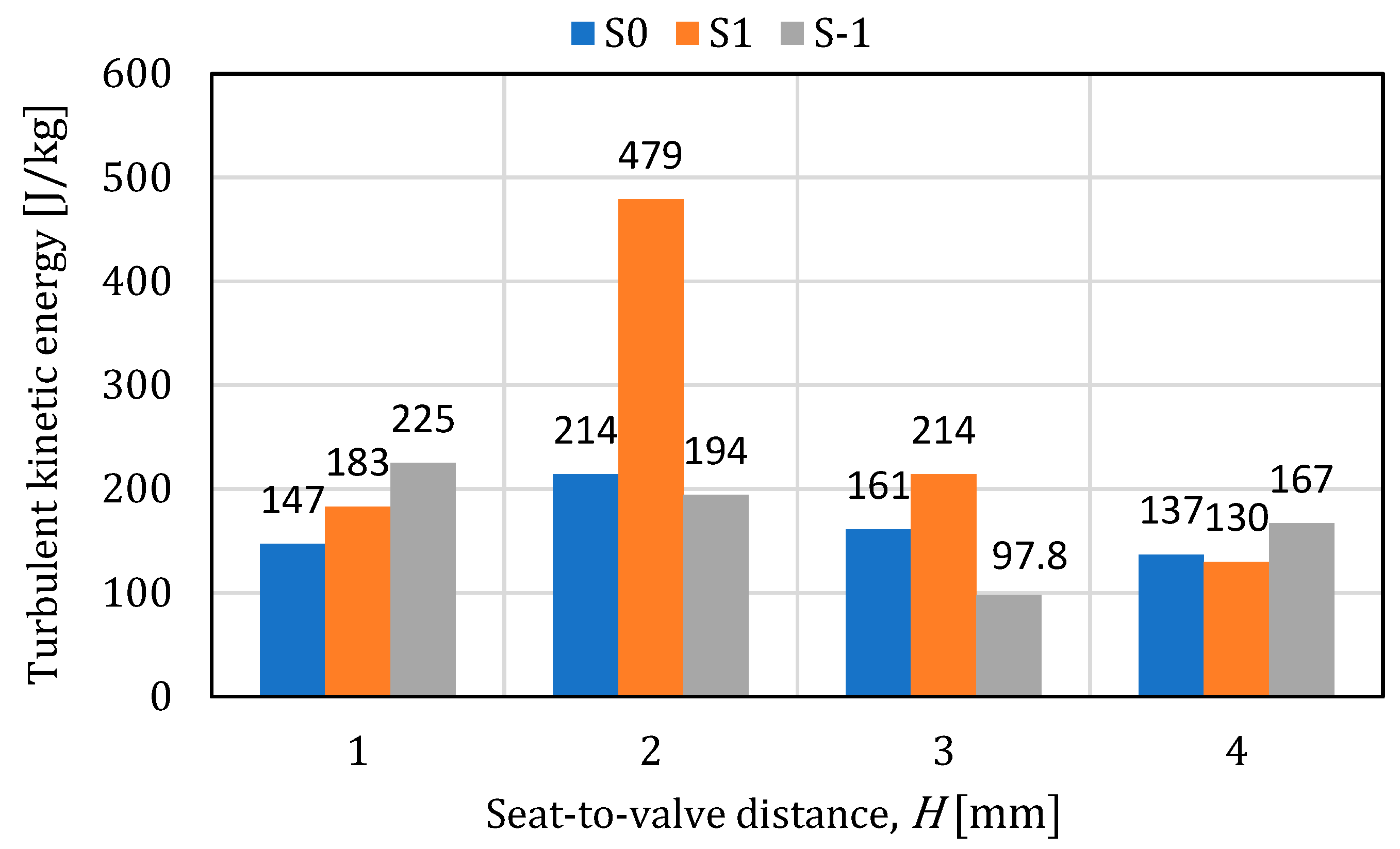
In case of water, the turbulent kinetic energy has a random distribution over the surface of both the plate and the seat. In the case of the plate, the maximum value is 5350 J/kg and was obtained in the S0-H2 situation. In the case of the seat, the turbulent kinetic energy has a relatively uniform variation for positions S0 and S-1, the highest value was obtained in the case of S1-H2 and is 479 J/kg.

4. Conclusions

In this paper, the analysis of the air/water flow through the Dn25/50-Pn40 discharge valve was carried out, using CFD simulation and considering four values of the seat–valve distance and three positions of the adjustment nozzle. Standards and norms, used by the manufacturers and operators of safety valves, do not specify the position of adjusting nozzle. Also, there are no studies regarding the correct position of the adjusting nozzle. This work establishes the proper position of the adjusting nozzle considering the main safety valve function—to avoid overpressure in the working system as quick is possible—with a maximum fluid velocity, and with a minimum turbulent kinetic energy. The study, applied to a Dn25/50-Pn40 safety valve, shows the importance of safety valve construction, working fluid and pressure for correct positioning of the adjusting nozzle.

The study utilized Computational Fluid Dynamics (CFD) simulations to analyze the air/water flow through the Dn25/50-Pn40 discharge valve. This suggests a reliance on numerical methods for understanding the fluid dynamics involved.

The analysis took into account four values of the seat–valve distance and three positions of the adjustment nozzle. This indicates a comprehensive investigation, exploring the impact of different configurations on the valve’s performance.

The focus on air/water flow implies a consideration of two-phase flow dynamics. Understanding how the valve behaves under different conditions with both air and water has implications for its applicability in diverse operational scenarios.

The variations in seat–valve distance and adjustment nozzle positions suggest a sensitivity analysis to evaluate how changes in these parameters affect the overall performance of the discharge valve. This information is crucial for optimizing the valve’s functionality.

The use of a Pn40 pressure class indicates that the valve is designed to handle relatively high-pressure conditions. This choice of pressure class is likely relevant to the specific applications for which the valve is intended. Analyzing the pressure distribution from Figure 25a and Figure 26a, some negative pressure contours can be observed, due the phenomenon of cavitation in the case of liquids, respectively, of compressibility; in the case of gases, phenomena do not interfere with the purpose of the article, namely to determine the optimal position of the adjusting nozzle depending on the value of the fluid velocity and turbulent kinetic energy.

The paper likely provides insights into the engineering aspects of discharge valves, offering valuable information for designers and engineers involved in fluid system design.

The performed statistical analysis showed that when dealing with air, the adjusting nozzle position stands out as the most critical factor regarding fluidvelocity, while for water, the seat–valve distance takes precedence. Moving on to the assessment of shear stress and turbulent kinetic energy, the analysis consistently highlights the seat–valve distance as the factor of greatest significance, for both air and water. These conclusions emphasize the essential role of specific variables in influencing fluid behavior and underline the importance of optimizing these factors to achieve desired outcomes in fluid flow and related parameters.

The optimization process has successfully identified the optimal combination of input parameters necessary to attain the desired outcomes in both air and water environments. For the air environment, the “greater is better” option for turbulent kinetic energy was achieved by setting S-1/H2, while the “smaller is better” option for turbulent kinetic energy was attained with the setting S0/H1. Similarly, in the water environment, the optimization process determined that the combination of S0/H2 results in “greater is better” turbulent kinetic energy, while S0/H1 is the ideal setting for “smaller is better” turbulent kinetic energy. These findings provide a clear and actionable roadmap for achieving the desired results in both environments, underscoring the importance of tailored parameter adjustments for specific conditions.

Therefore, this work provides valuable insights into the airflow dynamics within the examined valve, offering a comprehensive understanding of how different operational conditions influence its performance. The novelty of the performed research lies in the detailed examination of seat–valve distances and adjustment nozzle positions, revealing the complex interaction of variables within the valve, which has practical implications for valve optimization and design in various applications.

References

1. Scuro, N.L.; Angelo, E.; Angelo, G.; Andrade, D.A. A CFD Analysis of the Flow Dynamics of a Directly-Operated Safety Relief Valve. Nucl. Eng. Des. 2018, 328, 321–332. [Google Scholar] [CrossRef]
2. Dasgupta, K.; Karmakar, R. Dynamic Analysis of Pilot Operated Pressure Relief Valve. Simul. Model. Pract. Theory 2002, 10, 35–49. [Google Scholar] [CrossRef]
3. Prescott, S.L.; Ulanicki, B. Dynamic Modeling of Pressure Reducing Valves. J. Hydraul. Eng. 2003, 129, 804–812. [Google Scholar] [CrossRef]
4. Szpica, D.; Mieczkowski, G.; Borawski, A.; Leisis, V.; Diliunas, S.; Pilkaite, T. The Computational Fluid Dynamics (CFD) Analysis of the Pressure Sensor Used in Pulse-Operated Low-Pressure Gas-Phase Solenoid Valve Measurements. Sensors 2021, 21, 8287. [Google Scholar] [CrossRef]
5. Lisowski, E.; Filo, G.; Rajda, J. Analysis of Energy Loss on a Tunable Check Valve through the Numerical Simulation. Energies 2022, 15, 5740. [Google Scholar] [CrossRef]
6. Sun, Y.; Wu, J.; Xu, J.; Bai, X. Flow Characteristics Study of High-Parameter Multi-Stage Sleeve Control Valve. Processes 2022, 10, 1504. [Google Scholar] [CrossRef]
7. Song, X.; Cui, L.; Cao, M.; Cao, W.; Park, Y.; Dempster, W.M. A CFD Analysis of the Dynamics of a Direct-Operated Safety Relief Valve Mounted on a Pressure Vessel. Energy Convers. Manag. 2014, 81, 407–419. [Google Scholar] [CrossRef]
8. Alkhulaifi, K.; Alharbi, A.; Alardhi, M.; Alrajhi, J.; Almutairi, H.H. Comparative Analysis of the Performance Characteristics of Butterfly and Pinch Valves. Processes 2023, 11, 1897. [Google Scholar] [CrossRef]
9. Yang, L.; Wang, Z.; Dempster, W.; Yu, X.; Tu, S.-T. Experiments and Transient Simulation on Spring-Loaded Pressure Relief Valve under High Temperature and High Pressure Steam Conditions. J. Loss Prev. Process Ind. 2017, 45, 133–146. [Google Scholar] [CrossRef]
10. Makaryants, G.M. Fatigue Failure Mechanisms of a Pressure Relief Valve. J. Loss Prev. Process Ind. 2017, 48, 1–13. [Google Scholar] [CrossRef]
11. Yuan, G.; Wang, Y.; Fang, Y.; Ma, R.; Ning, K.; Tang, Y. High-Temperature and Pressure Downhole Safety Valve Performance Envelope Curve Study. Processes 2023, 11, 2525. [Google Scholar] [CrossRef]
12. Song, X.-G.; Park, Y.-C.; Park, J.-H. Blowdown Prediction of a Conventional Pressure Relief Valve with a Simplified Dynamic Model. Math. Comput. Model. 2013, 57, 279–288. [Google Scholar] [CrossRef]
13. Erdődi, I.; Hős, C. Prediction of Quarter-Wave Instability in Direct Spring Operated Pressure Relief Valves with Upstream Piping by Means of CFD and Reduced Order Modelling. J. Fluids Struct. 2017, 73, 37–52. [Google Scholar] [CrossRef]
14. Desai, S.; Desai, A.; Karande, V. Design and Weight Optimization of Buffer Relief Valve Using FEA with Experimental Validation. Mater. Today Proc. 2020, 27, 1466–1472. [Google Scholar] [CrossRef]
15. Hős, C.J.; Champneys, A.R.; Paul, K.; McNeely, M. Dynamic Behavior of Direct Spring Loaded Pressure Relief Valves in Gas Service: Model Development, Measurements and Instability Mechanisms. J. Loss Prev. Process Ind. 2014, 31, 70–81. [Google Scholar] [CrossRef]
16. Bazsó, C.; Hős, C.J. An Experimental Study on the Stability of a Direct Spring Loaded Poppet Relief Valve. J. Fluids Struct. 2013, 42, 456–465. [Google Scholar] [CrossRef]
17. Darby, R. The Dynamic Response of Pressure Relief Valves in Vapor or Gas Service, Part I: Mathematical Model. J. Loss Prev. Process Ind. 2013, 26, 1262–1268. [Google Scholar] [CrossRef]
18. Aldeeb, A.A.; Darby, R.; Arndt, S. The Dynamic Response of Pressure Relief Valves in Vapor or Gas Service. Part II: Experimental Investigation. J. Loss Prev. Process Ind. 2014, 31, 127–132. [Google Scholar] [CrossRef]
19. Darby, R.; Aldeeb, A.A. The Dynamic Response of Pressure Relief Valves in Vapor or Gas Service. Part III: Model Validation. J. Loss Prev. Process Ind. 2014, 31, 133–141. [Google Scholar] [CrossRef]
20. Karpenko, M.; Stosiak, M.; Šukevičius, Š.; Skačkauskas, P.; Urbanowicz, K.; Deptuła, A. Hydrodynamic Processes in Angular Fitting Connections of a Transport Machine’s Hydraulic Drive. Machines 2023, 11, 355. [Google Scholar] [CrossRef]
21. Stosiak, M.; Karpenko, M.; Deptuła, A.; Urbanowicz, K.; Skačkauskas, P.; Deptuła, A.M.; Danilevičius, A.; Šukevičius, Š.; Łapka, M. Research of Vibration Effects on a Hydraulic Valve in the Pressure Pulsation Spectrum Analysis. JMSE 2023, 11, 301. [Google Scholar] [CrossRef]
22. Stosiak, M.; Karpenko, M.; Prentkovskis, O.; Deptuła, A.; Skačkauskas, P. Research of Vibrations Effect on Hydraulic Valves in Military Vehicles. Def. Technol. 2023, in press. [Google Scholar] [CrossRef]
23. Budziszewski, A.; Thorén, L. CFD Simulation of a Safety Relief Valve for Improvement of a One-Dimensional Valve Model in RELAP5. Master’s Thesis, Chalmers University of Technology, Gothenburg, Sweden, 2012. [Google Scholar]
24. Singh, R.; Ahmed, R.; Karami, H.; Nasser, M.; Hussein, I. CFD Analysis of Turbulent Flow of Power-Law Fluid in a Partially Blocked Eccentric Annulus. Energies 2021, 14, 731. [Google Scholar] [CrossRef]
25. Leutwyler, Z.; Dalton, C. A CFD Study of the Flow Field, Resultant Force, and Aerodynamic Torque on a Symmetric Disk Butterfly Valve in a Compressible Fluid. J. Press. Vessel. Technol. 2008, 130, 021302. [Google Scholar] [CrossRef]
26. Leutwyler, Z.; Dalton, C. A Computational Study of Torque and Forces Due to Compressible Flow on a Butterfly Valve Disk in Mid-Stroke Position. J. Fluids Eng. 2006, 128, 1074–1082. [Google Scholar] [CrossRef]
27. Nazif, H.R.; Basirat Tabrizi, H. Applying a Non-Equilibrium Wall Function in k–ε Turbulent Modelling of Hydrodynamic Circulating Flow. Appl. Math. Model. 2014, 38, 588–598. [Google Scholar] [CrossRef]
28. Parente, A.; Gorlé, C.; van Beeck, J.; Benocci, C. Improved k–ε Model and Wall Function Formulation for the RANS Simulation of ABL Flows. J. Wind. Eng. Ind. Aerodyn. 2011, 99, 267–278. [Google Scholar] [CrossRef]
29. Nazif, H.R.; Basirat Tabrizi, H.; Farhadpour, F.A. Comparative Analysis of the Boundary Transfer Method with Other Near-Wall Treatments Based on the—Turbulence Model. Eur. J. Mech.—B/Fluids 2014, 44, 22–31. [Google Scholar] [CrossRef]
30. Nazif, H.R.; Tabrizi, H.B. Comparison of Standard Turbulent Wall Function with a Non-Equilibrium Wall Model. Inter. J. Fluid Mech. Res. 2011, 38, 499–508. [Google Scholar] [CrossRef]
31. El Gharbi, N.; Absi, R. Effect of Different Near-Wall Treatments on Indoor Airflow Simulations. JAFM 2012, 5, 63–70. [Google Scholar] [CrossRef]
32. Francis, J.; Betts, P.L. Modelling Incompressible Flow in a Pressure Relief Valve. Proc. Inst. Mech. Eng. Part E J. Process Mech. Eng. 1997, 211, 83–93. [Google Scholar] [CrossRef]
33. D’Addona, D.M.; Raykar, S.J.; Singh, D.; Kramar, D. Multi Objective Optimization of Fused Deposition Modeling Process Parameters with Desirability Function. Procedia CIRP 2021, 99, 707–710. [Google Scholar] [CrossRef]
34. Zisopol, D.G.; Tănase, M.; Portoacă, A.I. Innovative Strategies for Technical-Economical Optimization of FDM Production. Polymers 2023, 15, 3787. [Google Scholar] [CrossRef] [PubMed]
Figure 1. Shape and dimensions of the analyzed pressure relief valve: (a)schematic representation; (b) real shape.
Processes 11 03396 g001
Figure 2. Pressure valve subassemblies: (a)—the plate assembly; (b)—the seat assembly.
Processes 11 03396 g002
Figure 3. Fluid part of the3D model.
Processes 11 03396 g003
Figure 4. Determination of the elastic constant of the valve spring.
Processes 11 03396 g004
Figure 5. The elastic characteristic of the valve spring.
Processes 11 03396 g005
Figure 6. The mesh adopted in the CFD analysis of the valve.
Processes 11 03396 g006
Figure 7. Distance (H) between seat and valve.
Processes 11 03396 g007
Figure 8. Position of the adjusting nozzle: position S0 (a), position S1 (b), position S-1 (c).
Processes 11 03396 g008
Figure 9. Residual plots.
Processes 11 03396 g009
Figure 10. Air speed distribution.
Processes 11 03396 g010
Figure 11. Water speed distribution.
Processes 11 03396 g011
Figure 12. Air pressure variation in case of plate.
Processes 11 03396 g012
Figure 13. Water pressure variation in case of plate.
Processes 11 03396 g013
Figure 14. Shear stress variation in case of plate (air environment).
Processes 11 03396 g014
Figure 15. Shear stress variation in case of plate (water environment).
Processes 11 03396 g015
Figure 16. Turbulent energy variation in case of plate (air environment).
Processes 11 03396 g016
Figure 17. Turbulent energy variation in case of plate (water environment).
Processes 11 03396 g017
Figure 18. Air pressure variation in case of seat.
Processes 11 03396 g018
Figure 19. Water pressure variation in case of seat.
Processes 11 03396 g019
Figure 20. Shear stress variation in case of seat (air environment).
Processes 11 03396 g020
Figure 21. Shear stress variation in case of seat (water environment).
Processes 11 03396 g021
Figure 22. Turbulent energy variation in case of seat (air environment).
Processes 11 03396 g022
Figure 23. Turbulent energy variation in case of seat (water environment).
Processes 11 03396 g023
Figure 24. Airflow streamlines, case S0-H1: air (a); water (b).
Processes 11 03396 g024
Figure 25. CFD results for plate, (case S0-H1): pressure (a), shear stress (b), turbulence kinetic energy (c).
Processes 11 03396 g025aProcesses 11 03396 g025b
Figure 26. CFD results for seat, (case S0-H1): pressure (a), shear stress (b), turbulence kinetic energy (c).
Processes 11 03396 g026aProcesses 11 03396 g026b
Figure 27. Pareto Charts for fluid velocity: (a) air; (b) water.
Processes 11 03396 g027
Figure 28. Pareto Charts for shear stress: (a) air; (b) water.
Processes 11 03396 g028
Figure 29. Pareto Charts for turbulent kinetic energy: (a) air; (b) water.
Processes 11 03396 g029
Figure 30. Main effects plot for fluid velocity: (a) air; (b) water.
Processes 11 03396 g030
Figure 31. Main effects plot for shear stress: (a) air; (b) water.
Processes 11 03396 g031
Figure 32. Main effects plot for turbulent kinetic energy: (a) air; (b) water.
Processes 11 03396 g032
Figure 33. Multi-response optimization plots in case of air environment: (a) “greater is better” for TKE, (b) “smaller is better” for TKE.
Processes 11 03396 g033
Figure 34. Multi-responseoptimizationplots in case of water environment: (a) “greater is better” for TKE, (b) “smaller is better” for TKE.
Processes 11 03396 g034