1. Introduction
Methanol is a widely used and important raw material for the chemical industry [
1,
2]. It can also be used for chemical energy storage [
1,
3]. Today, methanol is produced large-scale using fossil-based synthesis gas in heterogeneously catalyzed reactions. The worldwide annual production is 98 million tonnes [
4]. Of that, only a small fraction, i.e.,
million tonnes, is produced from renewable resources [
4]. In the light of climate change, it becomes clear that green methanol will play an important role [
5,
6]. For the production of green methanol, the fossil-based raw materials need to be substituted by renewables. Possible carbon sources are, among others, biogas [
7,
8], industrial fumes [
9], and direct CO
air capture [
10]. A suitable hydrogen source is electrolysis using electricity produced by solar, wind, or water power [
8,
11]. Due to the transformation of the energy supply system, there are already a number of pilot-scale plants for the production of green methanol in operation [
12]. However, as of today, the costs for renewable methanol are still much higher than for its fossil counterpart. This might change in the future due to legislation or more efficient processes [
11,
13,
14].
One of the challenges in the production of green methanol is to cope with fluctuations in the feed streams [
15,
16,
17], e.g., a varying availability of regenerative electricity and hence hydrogen. Conventional processes are operated under steady-state conditions with little to no fluctuations [
2], therefore they can be operated very efficiently. For the design of green processes, the fluctuations need to be taken into account and hence the processes need to be more robust, i.e., the possible window of operation needs to be bigger. Robustness always comes with sub-optimality in a sense that the design needs to be more conservative [
18]. This problem can be tackled by means of a multistage reactor design, as shown by Fischer et al. for methanation processes [
19,
20]. In the present paper, this concept is explored for methanol production.
This study aims at the robust optimization [
18,
21] of the operating conditions of a multistage reactor, consisting of three continuously stirred tank reactors, for the production of green methanol, where fluctuations in the hydrogen supply are taken into account. As stated above, a robust design always leads to conservative processes. Furthermore, neglecting the dynamic behavior of the process during robust optimization may lead to infeasible dynamic processes due to transient effects. A feed-forward control scheme consisting of a dynamic optimization in a short time horizon is proposed to overcome this limitation by manipulating the feed distribution and the shell temperatures.
The paper is structured as follows: The required model equations, assumptions, parameters, and the optimization problems are presented in
Section 2. The obtained results are shown and discussed in
Section 3. Finally, a short summary of the study, the results, and concluding remarks are given in
Section 4.
2. Materials and Methods
The process investigated in this work is a heterogeneously catalyzed methanol synthesis using a conventional Cu/ZnO/Al
2O
3 catalyst. The process is widely used in industry, with operating conditions between [50, 60] bar and around 250 °C, typically in fixed-bed reactors [
2,
22,
23].
2.1. Kinetic Model
The following three overall reactions take place:
where Equation (1) is the CO hydrogenation, Equation (2) is the CO
hydrogenation, and Equation (3) is the water gas shift reaction.
Established catalysts and kinetics are efficient for feeds consisting mainly of CO, which is also applied in this paper. This implies a two step process, where first CO
2 is converted to CO, which is then converted to methanol [
24].
The reaction kinetics is taken from Seidel et al. [
25,
26], with parameters taken from [
27] and given in
Table 1. It is modeled as a Langmuir–Hinshelwood kinetics with three types of catalyst centers: heterolytic (het), reduced (red), and oxidized (oxi). The availability of those centers depends on the oxidization state of the catalyst,
. As different centers are necessary for the three reactions, there is a direct influence of the catalyst state on the reaction rates
,
where
are the partial pressures of components
,
are temperature dependent equilibrium constants,
and
are temperature dependent reaction rate constants for reactions
,
with
K. The relative number of available catalyst centers can be calculated with
The parameters
were fit to experimental data by Seidel et al. [
27]. Note that terms with parameters equal to 0 in [
27] are neglected here. For a refit of the kinetics, the full version would be required.
Finally, the differential equation to describe the oxidization state of the catalyst reads
where
are the mole fractions of component
i,
, and
The kinetics were fitted to steady-state and dynamical experiments conducted in a micro-Berty reactor. This reactor type resembles a good approximation of an ideally mixed continuous stirred tank reactor (CSTR).
In contrast to traditional kinetic models for methanol synthesis [
28,
29,
30], dynamic changes of the catalyst are taken into account (Equation (
12)), therefore the model is also able to reproduce the transient behavior [
25].
2.2. Reactor Model
We consider a non-isothermal CSTR under constant pressure. In the following description of the reactor model, the species are denoted by subscripts
i and
k, the reactions are denoted by subscript
j. The gas and solid phases are denoted by superscript G and S, respectively. The derivation of the material balances follows that of Seidel et al. [
27] closely. However, note that in the present work the temperature also changes with time, hence the equations have to be adopted accordingly.
We start with the component material balance,
with,
where
are the molar fractions,
are the stoichiometric coefficients, the reactor’s pressure, volume, and temperature are given by
,
, and
T, respectively,
is the volumetric outlet flow-rate,
is the feed flow rate,
is the feed temperature,
is the catalyst mass,
is the adsorption capacity of the catalyst, and
are competitive Langmuir adsorption isotherms, which depend on the partial pressures of the species. Details are given in [
31]. The reactor temperature
T is equal to the outlet temperature, hence the subscript “out” will be neglected for better readability. Note that all
in Equation (18) not used in Equations (9)–(11) are equal to 0.
The time derivatives for
, and
are given by
an explicit calculation of the partial derivatives of the adsorption isotherms,
, can be found in the Appendix of Nikolić et al. [
31].
Introducing Equations (19) and (20) into Equation (14),
and summation over the single species yields the total material balance,
Solving Equation (
22) for
to eliminate it in Equation (
21) yields the component material balance in its final form,
Note that Equation (
23), in contrast to Equations (
21) and (
22), is identical to that obtained assuming a constant reactor temperature [
27], i.e., the component material balance is not temperature-dependent. However, the volumetric outlet flow rate (which can be derived from Equation (
22)) differs, as it is temperature dependent,
2.3. Energy Balance
To describe the change in temperature, an energy balance is required. We start with the total energy balance,
where
are enthalpies, and
is the cooling. Applying the product rule, introducing
, and assuming constant
, and
yields
To simplify the equation, the component material balance, Equation (
14), is multiplied with the component gas enthalpies,
, summed over
i, and solved for
where
is the heat of reaction
j. Putting this into Equation (
26) yields
The enthalpies can be described by
where
is the heat of formation and
is the isobaric heat capacity. We assume that
does not depend on the temperature, a correlation for
in J mol
K
,
as well as values for
and
, given in
Table 2, can be found in [
32].
With that, and by introducing the heat of cooling, the following equation can be obtained for the change in temperature:
with
The adsorption enthalpy is assumed to be constant and identical for each component, with J mol. Note that, since the heat of adsorption is relatively small compared to the heat of reaction, only a rough estimate is used.
2.4. Multistage Reactor
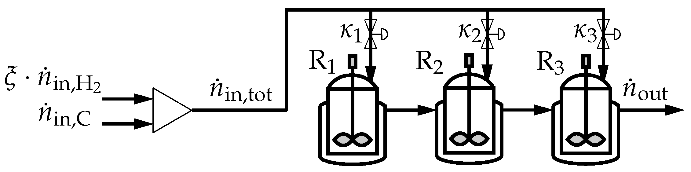
The considered process is depicted in
Figure 1. The multistage reactor consists of three CSTR with side-feeds for each reactor, which can be seen as an approximation of a staged multibed reactor. For CO
2 methanation, it is demonstrated in [
19,
20] that such a feed split increases robustness against fluctuations. The idea is transferred here to methanol production from CO. A different concept of a staged fixed bed reactor for methanol production from CO
2 was studied by Torcida et al. [
33]. There, intermediate cooling without feed split between the different stages is used to increase reactor efficiency.
We consider 3 reactors within the setup; they will be denoted by the subscript in the following.
The feed is split by a split-ratio,
, with
where
is the total volumetric inlet flow into the system. It consists of the fluctuating hydrogen stream,
, and a carbon stream,
, its composition and amount is calculated with
The inlet compositions and temperatures for reactors 2 and 3 are calculated accordingly with
where
is the temperature of the inlet into the system. Note that the inlet temperature and inlet composition for stage
are mean values based on the mole amounts of the entering streams, hence those values are estimates.
The reactors are parameterized such that the overall system resembles an industrial scale reactor. The heat transfer coefficient,
, was approximated according to [
34,
35]. The parameters are given in
Table 3. The overall reactor volume and catalyst mass are split equally,
2.5. Optimization Approach
We consider three optimization problems. The first one is the nominal steady-state optimization problem,
where
are variables with upper (
) and lower bounds (
). The space–time yield is defined as
and the carbon conversion is defined as
upper and lower bounds for the variables are given in
Table 4. We enforce a specific carbon conversion rate, while carbon conversion and the objective of a maximized space–time yield are concurrent. This also leads to higher reactor temperatures, as the reaction is exothermic. To prevent hotspot formation, there is a restriction on the differences between the reactor temperatures and the shell temperatures in Problem 1 (
44) [
36].
The second problem is the robust steady-state optimization,
where the space–time yield is maximized with the same constraints as in Problem 1 (
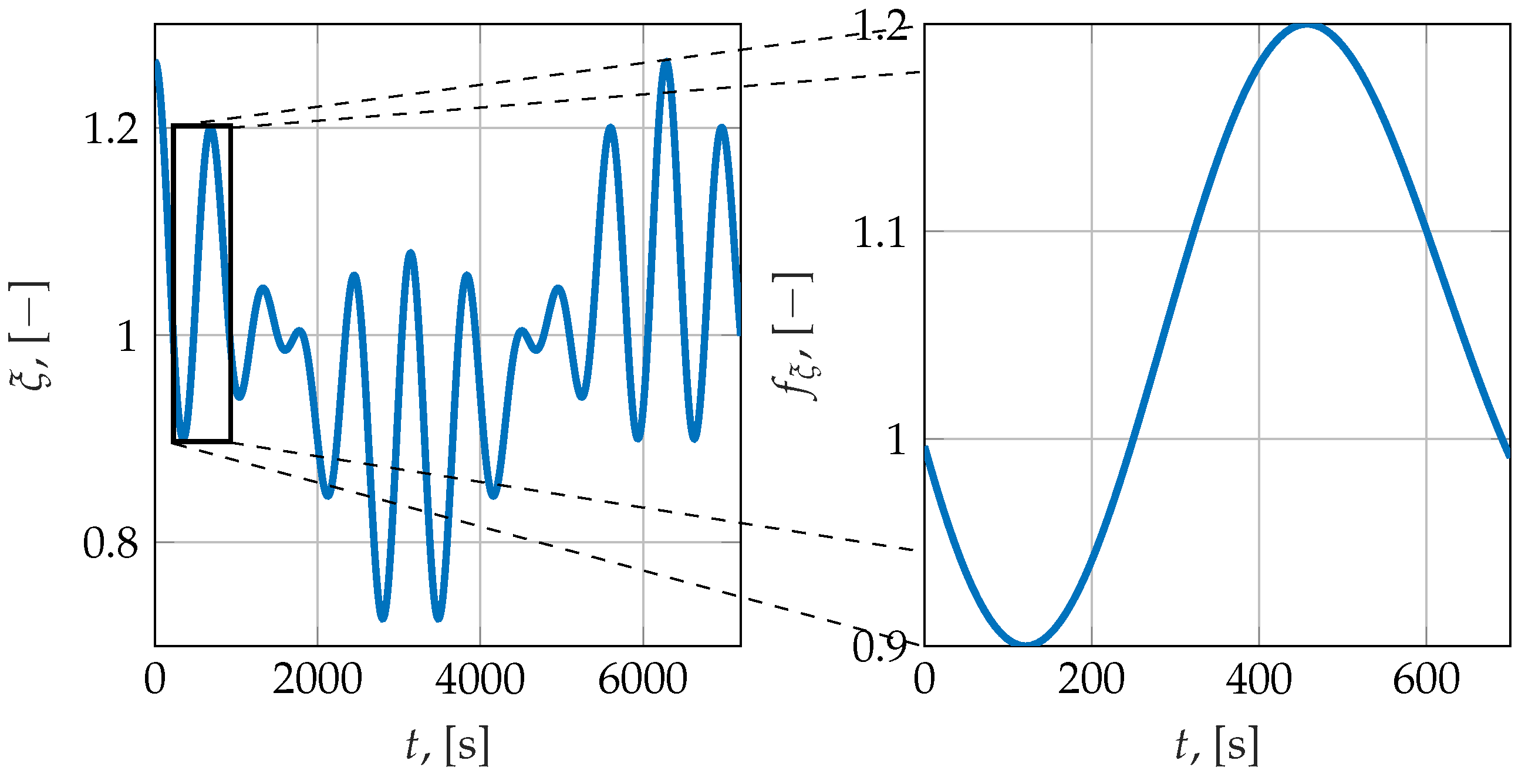
44), but with taking fluctuations into account (see the left plot of
Figure 2):
is the disturbance of H
2 at the inlet, the problem is discretized along
using 50 equally distant distributed support points. It is assumed that the carbon source is able to deliver CO and CO
2 as needed, but the hydrogen source is prone to fluctuations due to its renewable character, i.e., hydrogen is produced via electrolysis using wind energy. Each support point of
refers to a different scenario with a given disturbance rate. The problem is solved simultaneously, i.e., the optimizer identifies an optimal solution that holds the constraints for each support point of
.
Note that we only consider steady-state scenarios of the process here. Transient behavior that may occur when changing from one disturbance to another is neglected in this step.
The third optimization problem is a dynamic optimization, where the design parameters of the reactor setup are fixed. Only operating conditions, i.e., the feed split and the shell temperatures, may be changed dynamically. The problem is defined as:
where
are slack variables, and
is a heuristically set penalty constant. The slack variables allow for violation of the constraints at the expense of a highly reduced cost function, hence the optimizer tries to avoid this as much as possible.
Note that additional constraints are present in Problem 3 (
48) to determine the dynamic behavior of the feed split and shell temperature. First order lag equations are used to obtain a more realistic result, with time constants of 15 and 50, respectively. Without those lags, the optimizer would be able to change the operating conditions instantly from one extreme to another in the feasible range, giving rise to so-called bang-bang solutions. Although bang-bang solutions may be optimal, they are not achievable in a real application. Variables
, and
are the setpoints of the lag elements, which are degrees of freedom for the optimizer.
All optimization problems are implemented in Julia [
37], using the JuMP [
38] based package InfiniteOpt [
39]. For Problem 3 (
48) an orthogonal collocation of third order [
40] with 200 equally distant support points is used for the discretization of the infinite dimensional problem. All three problems are solved using the NLP solver KNITRO [
41]; for Problems 1 (
44) and 2 (
47), the multi-start option is set to 50.
2.6. Test Function
A drawback of Problem 2 (
47) is that only steady-state realizations are investigated, neglecting the transient behavior when fluctuations occur. The design obtained from Problem 1 (
44) does not take fluctuations into account. Therefore, an additional test is required to check whether the imposed constraints are met under dynamically changing disturbances. The employed test function is depicted in the right subplot of
Figure 2. It can be described by the following set of equations,
where
is the imaginary number, and
is the real part of
f. The time is shifted such that
. The test function can be interpreted as a complex Fourier series, which is truncated after the third entry and normalized such that the resulting function lies within the desired interval.
Note that the employed test function for dynamic transient behavior does not resemble the worst-case scenario, which would be a series of rectangle steps. Instead, it is modeled such that it resembles real wind fluctuations [
42,
43] better. However, the presented disturbance fluctuates more rapidly than it would be observed in the real world. Hence, it is a model profile not related to an existing green electricity profile. A short time horizon of this modeled disturbance was arbitrarily chosen as the test function, marked with a black rectangle in the left plot of
Figure 2.
The test function is used in a dynamic forward simulation of the obtained reactor setups from Problems 1 (
44) and 2 (
47), starting at the steady-state of the system.
A linear interpolation is used for the simulation of the design obtained from Problem 2 (
47). The feed split ratios in between the support points are interpolated.
The simulation is implemented in Julia using the DifferentialEquations [
44] package.
3. Results and Discussion
Two case studies are discussed in this section, one with the nominal reactor obtained from Problem 1 (
44) and one with the robust reactor obtained from Problem 2 (
47). Both reactor realizations are tested in a simulation framework and are compared to each other. In a last step, the dynamic optimization in Problem 3 (
48) is solved for both designs.
3.1. Nominal Steady-State Design
The nominal design is the solution of Problem 1 (
44). The obtained optimal values of the degrees of freedom are given in
Table 5.
The lowest possible inlet temperature is chosen. As the reaction is exothermic, the inlet stream acts as a sort of cooling mechanism.
The inlet stream consists mostly of hydrogen, with . Note that this value lies on the boundary. If no restriction on is present, the value is chosen to be higher, which would be favorable for the temperature management of the reactor setup. However, most of the increased hydrogen stream would leave the reactor unreacted, increasing the overall process cost.
Regarding the feed split, approximately one fifth of the feed is fed into the first reactor and four fifths are fed into the second. The first reactor is relatively cold, which leads to a fast conversion and a high temperature increase; therefore, only a small fraction of the reactants can enter. With increasing temperature, the reaction and heat production slow down. Therefore, most of the feed is fed into the much hotter second reactor, which is not only cooled by the shell, but also by the entering streams. The feed to the third reactor is not used. Feeding the third reactor would reduce the residence time, as the first two reactors are bypassed. This would lead to the production of less methanol, which is unfavorable for the used objective function.
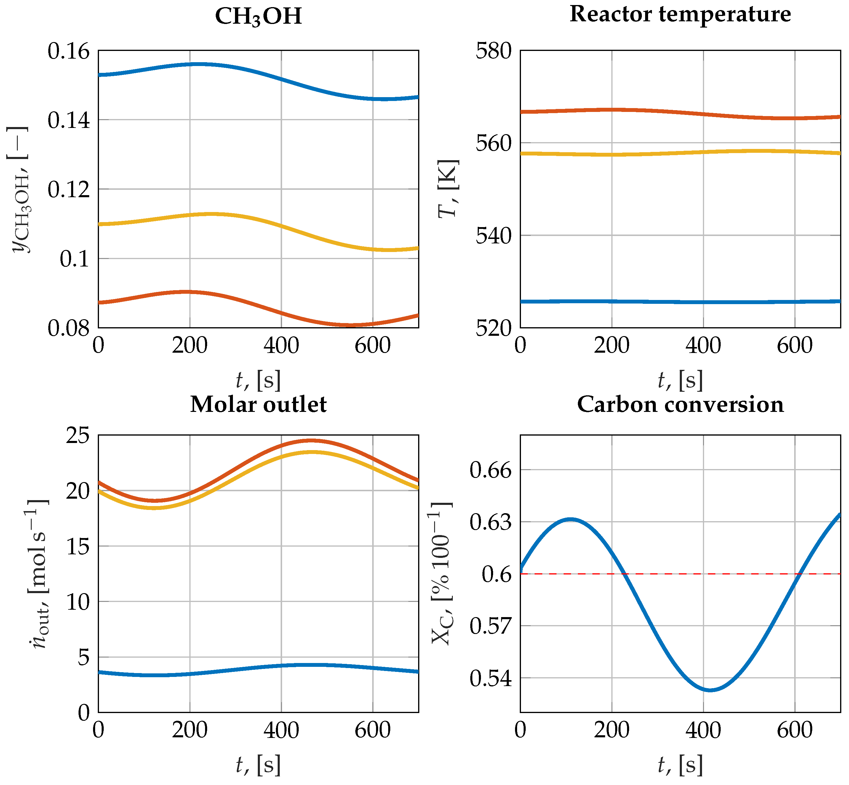
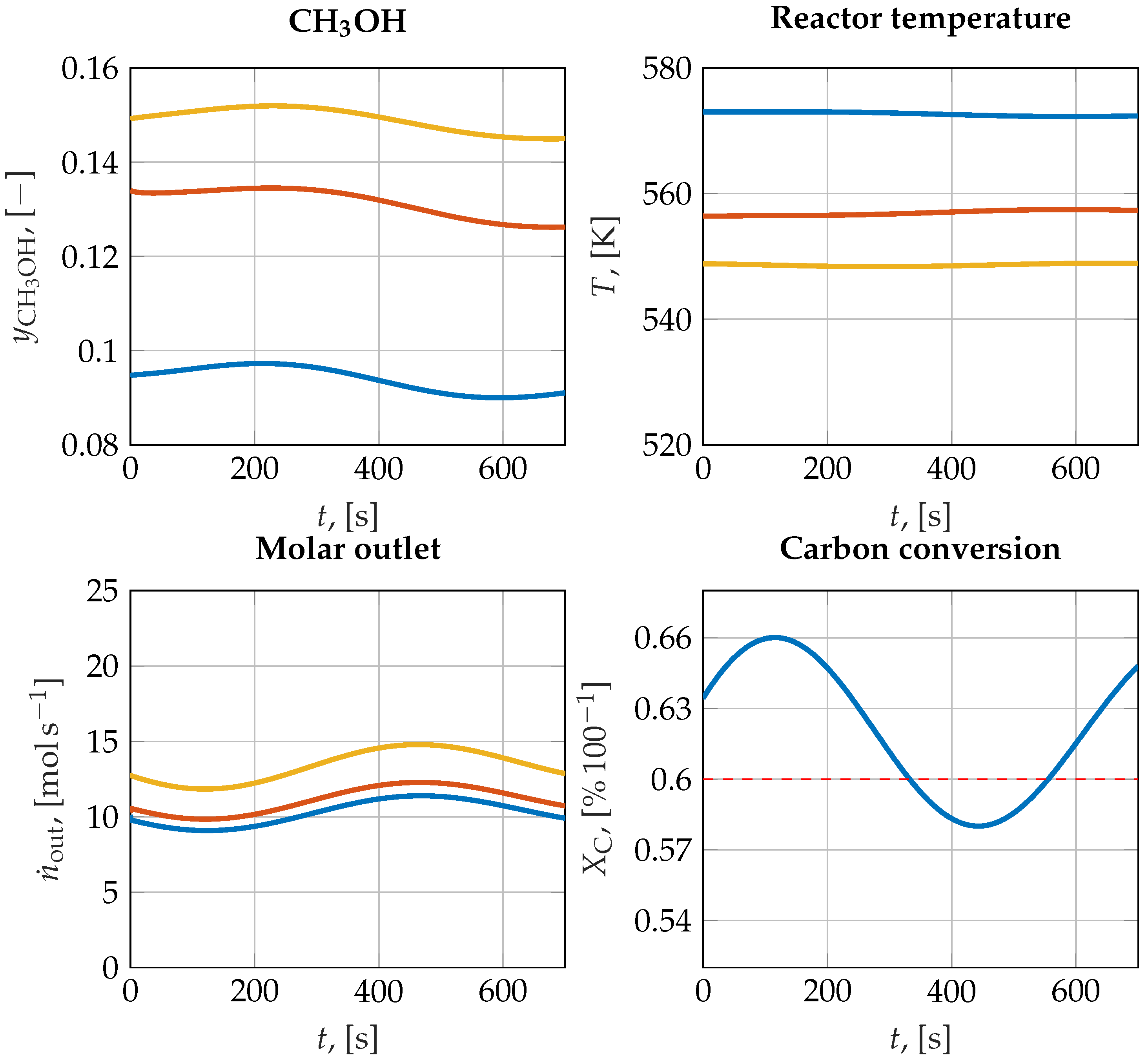
The dynamic simulation results for the nominal reactor design are shown in
Figure 3. The figure consists of four subplots: the upper left corner shows the mole fraction of methanol over time, the upper right corner the reactor temperature over time, the lower left corner the molar outlet streams over time, and the lower right corner the carbon conversion rate over time. The fluctuations can be well observed in all of those subplots. It is clear from the lower right subplot that the nominal reactor is not feasible for the present disturbance, as it lies well below the desired carbon conversion of 60%. The obtained space–time yield is
.
3.2. Robust Design
The robust design is the solution of Problem 2 (
47). The obtained values of the constant degrees of freedom are given in
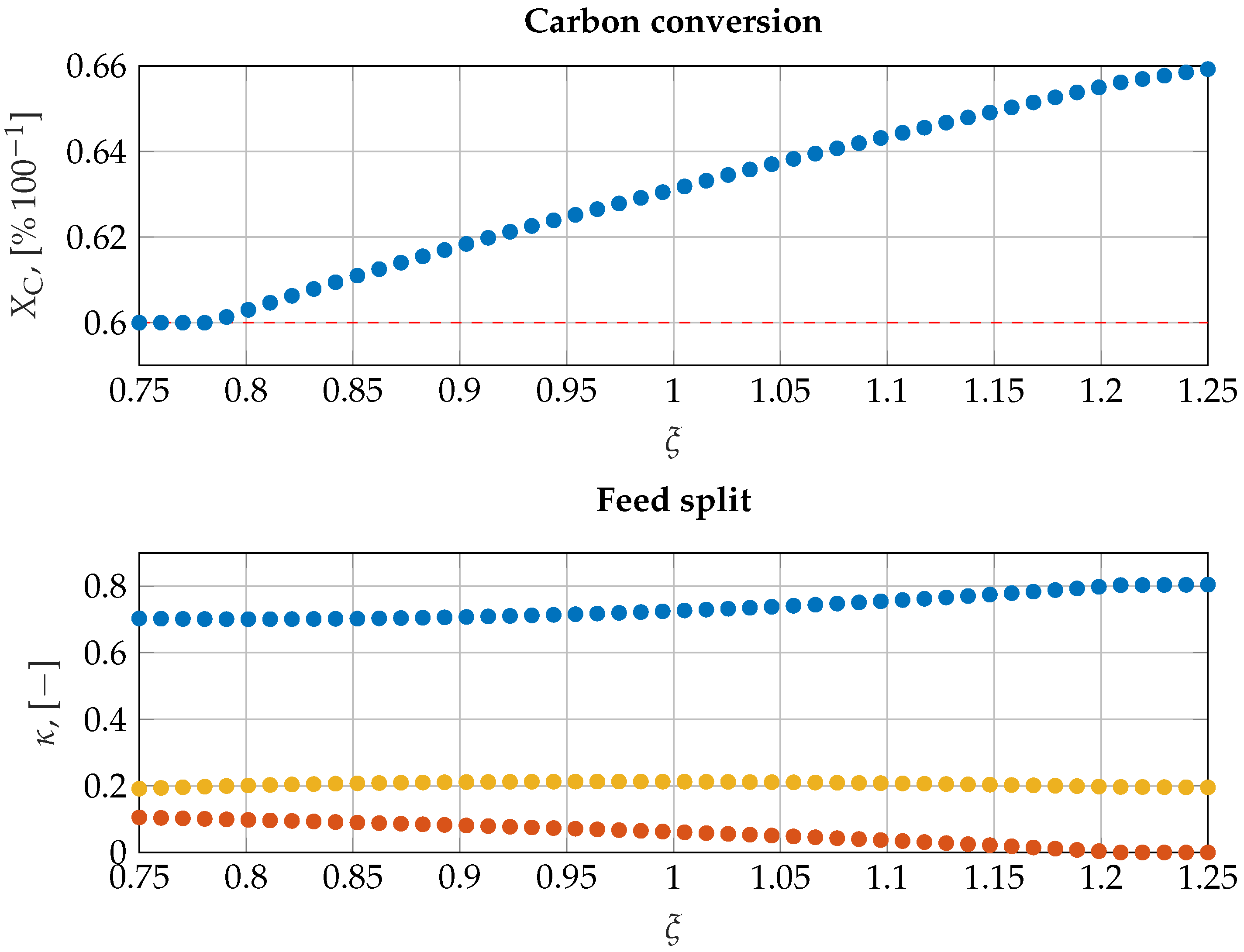
Table 6,
Figure 4 shows the feed split and the resulting carbon conversion rates. Note that the
x-axis of
Figure 4 is the disturbance.
The inlet composition is slightly different than for the nominal case. There is proportionally less H2 fed into the reactor. However, the obtained value for leads to a mole fraction of 0.85 for the highest hydrogen inlet increase. There is also slightly more CO2 present in the inlet stream.
The inlet temperature is, again, chosen to be as small as possible. There is a notable difference between the shell temperatures chosen for the nominal and robust designs. While the shell temperature of the first reactor in the nominal design is very low, it is the highest in the robust design. This can be explained by the feed split. In contrast to the nominal design, most of the feed is fed into the first reactor now.
The feed split changes for different disturbance values, although its main split remains constant: most of the feed goes into reactor 1. Interestingly, some of the feed is fed directly into reactor 3. Note that reactor 3 is the coldest and hence has the fastest reaction rate.
Generally, with increasing hydrogen flows, the steady-state carbon conversion increases and vice versa, as the temperature is reduced by a higher inlet flow, which increases the reaction rate due to the temperature dependence of the equilibrium of the water-gas-shift reaction.
Compared to the nominal design, the mean space–time yield of the robust design is reduced by 14%. This is to be expected, as the robust design has to be more conservative and hence inefficient.
The dynamic simulation results for the robust reactor design are shown in
Figure 5 (the figure has the same layout as
Figure 3, described above). Although much better than in the nominal case, the robust design is still infeasible with regard to the carbon conversion, as it lies below the desired 60%. This can be explained by the neglected transient behavior and non-linear dynamics of the model, as Problem 2 (
47) only considers a steady-state optimization. The obtained space–time yield is
, which is 12.6% less than in the nominal case and the price we have to pay for the increased robustness.
3.3. Dynamic Optimization
The dynamic optimization is the solution of Problem 3 (
48).
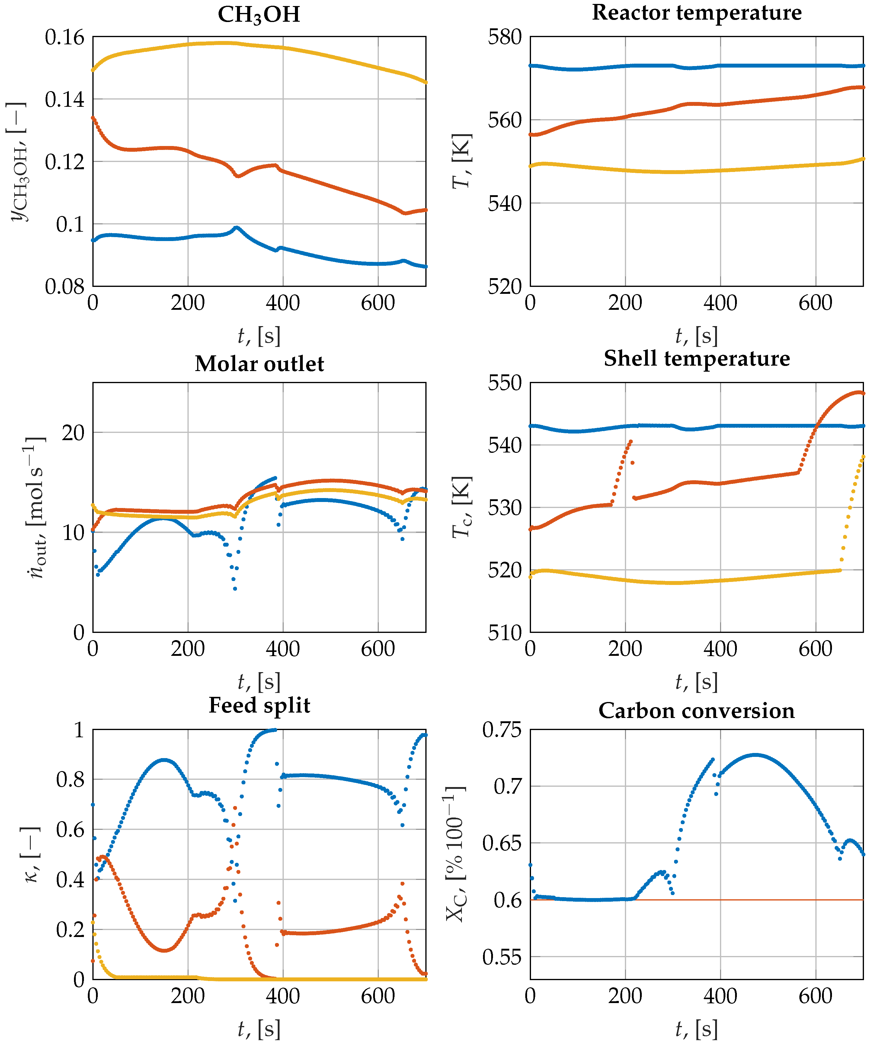
The result for the robust design is shown in
Figure 6, where the collocation support points are plotted.
The feed split ratios are chosen differently than for the robust steady-state design. The feed bypass to the third reactor is completely shut down, while the second reactor gets more of the feed stream. For the first reactor, the value of the split is mostly close to that of the steady-state design, except for some drastic dynamic changes between 300 and 400 s, and 636 and 700 s. The first interval is located in the region where the simulation of the steady-state design became infeasible. Therefore, the optimizer has to choose a different control to achieve feasibility. The second interval comes due to the absence of terminal constraints, the objective function is increased by maximizing the output. In a practical application, the optimization would be repeated before this interval is reached.
The achieved space–time yield is , which is slightly below that of the robust case. It is, however, feasible.
The dynamic optimization for the nominal design converges to an infeasible point. The optimizer is not able to control the process such that the reactor temperatures remain within their bounds.
4. Conclusions
Methanol synthesis is a crucial topic in light of the upcoming changes in energy supply. As traditional steady-state processes will have to cope with energy fluctuations, they will also have to deal with fluctuations in their operating conditions. In this paper, we have investigated the influence of fluctuations on the inlet flow of a staged methanol synthesis reactor.
To address this challenge, both a nominal and a robust steady-state optimization of the reactor setup’s operating conditions were conducted. As expected, the obtained optimal nominal reactor has a better performance than the robust reactor, which has to be more conservative in its design. However, for both designs, the dynamic behavior of the process was neglected, i.e., only steady-state optimizations were conducted. To take the transient behavior into account, both designs were tested with a predefined disturbance function. While the robust reactor is able to hold the imposed constraint on carbon conversion for a longer period, it ultimately also operates in an infeasible area.
In our case study, the disturbance is caused by fluctuating wind conditions. These wind conditions can be measured and predicted within a short time horizon. This provides an opportunity for a control scheme via dynamic optimization. To ensure feasible operation, an additional dynamic optimization was performed using fluctuation-specific split ratios and shell temperatures as degrees of freedom. While the nominal design converges to an infeasible point, the optimizer is able to control the operating conditions such that the robust reactor becomes feasible. Of course, the results depend on the imposed fluctuation function: its respective upper and lower bounds, as well as its dynamics. In a real application, additional buffer tanks would be used to make sure that the fluctuations exhibit desirable characteristics. Those tanks could also be included in the optimization problem to account for the buffer costs, which is, however, not the scope of this paper.
The approach presented in this paper can be interpreted as a feed-forward control scheme. In future works, we plan to enhance the dynamic optimization step used for calculating the control action with a machine learning-based approach [
45]. For disturbances beyond the considered scenarios, an additional buffer tank for H
2 would be required. Simultaneous optimization of reactor and buffer designs under dynamic conditions is another interesting topic for future work. Furthermore, we intend to augment the overall control scheme with a feedback loop or, alternatively, conduct repetitive online optimizations to account for additional disturbances and plant model mismatch. The number of stages used in the present work was chosen exemplarily. Further work will be concerned with finding the optimal amount of stages for different scenarios. Additionally, the CSTRs will be replaced by industrially more relevant fixed bed reactor segments
In conclusion, this paper presents a novel approach to addressing the challenge of fluctuations in feed streams for methanol synthesis from renewable feedstock. By combining robust optimization with dynamic optimization, we have demonstrated that it is possible to generate a reactor design that is dynamically feasible for measurable fluctuating inlet conditions in a limited range.


