
Analysis of the Flow Field at the Tip of an Axial Flow Compressor during Rotating Stall Process Based on the POD Method
School of Mechanical Engineering, Shanghai Jiao Tong University, 800 Dongchuan RD. Minhang District, Shanghai 200240, China
*
Author to whom correspondence should be addressed.
Processes 2023, 11(1), 69; https://doi.org/10.3390/pr11010069
Submission received: 26 October 2022
/
Revised: 21 December 2022
/
Accepted: 23 December 2022
/
Published: 27 December 2022
(This article belongs to the Special Issue Advanced Simulation and Experiment Methods of Flow Instability in Hydraulic Machinery)
Abstract
:Rotating stalls are one of the most dangerous phenomena to be avoided in the designing and operating of axial flow compressors. An understanding of the evolution of the flow characteristics around the rotor tip region is important to study the process of stall development. In this paper, some critical characteristics of the stall-related structures, which could not be observed by the traditional analysis methods, are understood by using the proper orthogonal decomposition (POD) method. The detailed unsteady flow fields in a typical transonic axial flow compressor during the stall process are obtained by the validated numerical simulation. Thereafter, the proper orthogonal decomposition method, as a method for model reduction and decomposition, is adopted to extract the flow characteristics from the numerical results of the stall process. It is found that the flow characteristics during the stall process can be well decomposed by the POD method. The pre-stall POD results show that the important flow features can be extracted and revealed in the low-order modes, which are not obvious in the original flow field. When the stall cells are formed and developed, the flow characteristics are gradually determined by the modes, which are related to the features of the stall cells. When the compressor is operated under stable stall conditions, the low-order POD modes are composed of a series of harmonic modes, which are sinusoid-like in space and time with the frequency of the stall cell rotation.
1. Introduction
Rotating stall is one of the most common types of circumferentially non-uniform and unsteady flow phenomenon in an axial flow compressor [1]. Its dangerous aerodynamic effects can induce surge step by step and then lead to fatigue fracture of the compressor blades [2].
The rotating stall has a profound connection with the high flow complexity in the rotor tip region and leads to the aerodynamic loss in the rotor tip region, which accounts for more than 30% of total losses [3]. In 1993, Adamczyk et al. [4] focused on this kind of flowing complexity and conducted a numerical simulation of the transonic axial flow compressor, NASA Rotor67. They found that when the mass flow rate was gradually decreased, the migration path of the tip clearance vortex (TCV) was deflected circumferentially along the axial direction. This in turn resulted in a forward movement of the blockage area induced by the shock wave and TCV, and eventually brought the compressor into stall condition. When the compressor was trapped in these conditions, divergence in the numerical calculation was unavoidable. Yamada et al. [5] performed unsteady numerical calculations for the NASA Rotor37 and revealed the relationship among the stall, the tip leakage flow, and the shock wave at the blade tip.
In our experience, the stall process can be divided into three stages, such as stall inception (called pre-stall), stall cell formation (called during-stall), and stable stall [6]. In general, it is believed that there are two main types of stall inception, such as the large-scale modal-type and the small-scale spike-type [7]. The waves of the former type are large in scale but small in amplitude and developed along the circumferential direction. They gradually are increased in strength before stall, and finally developed into several stall cells within a few tens of revolutions. However, spike-type waves are those small in scale but large in amplitude with higher non-linearity [8]. Hah et al. [9] used large eddy simulation (LES) with a full-flow channel model to study the stall inception of a transonic compressor. They found that the unsteady oscillation of the channel shock wave and the TCV could result in spike-type waves at the stall inception. According to the research of Pullan G et al. [6], spike-type waves could be regarded as the embryonic of stall cells. They continuously were spread in the direction opposite to the rotating direction from small-scale disturbances to large-scale stall cells. Once stall cells formed, they would rotate with a speed certain ratio of blade rotor speed. The physical mechanism for how determining the speed of stall cell had not been completely understood yet, but Day’s study [2] showed that some geometrical parameters related to inlet guide vane (IGV) had a more significant effect on the stall cell speed than other geometrical features. The theory of the three stages of the stall process is meaningful to the understanding of the stall, but it is very difficult to distinguish and conclude the most effective characteristics of the three stall stages respectively by the traditional method. So, researchers need to adopt new methods to do with the data of the stall process.
The proper orthogonal decomposition (POD) method may be an alternative and effective method to distinguish some critical features from lots of data, which makes it possible to understand and analyze the unsteady stall flow field more accurately [10]. The POD method was first introduced by Lumley [11] in 1967 for the analysis of the coherent structure of turbulent flows. The POD method could decompose complex data into basic modes with reduced dimensions. The decomposed modes were ordered by energy proportion, and the flow features shown in low-order modes could be regarded as the ones, which influence the flow field greatly [12]. It was due to its advantages that some researchers made their efforts on its applications. Aubry and Ma et al. [13,14] analyzed the boundary layer of flat plate and flow around circular cylinders by using the POD method. In 2015, Wu et al. [15] focused on the 3D flow field of wind turbine blades and analyzed the statistical impacts of large-scale and energetic structures on turbulence. Mallik and Raveh in 2020, presented an investigation of light dynamic stall phenomena on a pitching NACA 0012 airfoil via the POD method [16].
In summary, many researchers had paid attention to the POD method and adopted it as a useful method to reduce data dimension. So, the POD method and its applications had been improved greatly. However, there were seldom publications to describe the application of the POD method on the rotating stall process in an axial flow compressor. The POD method has the ability to decompose flow characteristics into different POD modes according to their influence on the flow field. Compared with the methods of analyzing the unsteady original flow field, the POD method can grasp some critical characteristics, which can not be observed by the published works, so that the rotating stall process can be understood more directly and accurately. Therefore, in this paper, the POD method has been adopted to decompose the flow field during the rotating stall process obtained from the unsteady numerical simulation of a transonic axial flow compressor. Subsequently, in order to explore the flow patterns, the mode characteristics of the three stall stages have been distinguished and analyzed.
2. Proper Orthogonal Decomposition Method
For the proper orthogonal decomposition (POD) method, a set of physical quantities that are continuous in time and space are decomposed [17]. The decomposed result is an optimal orthogonal subspace which is composed of basic functions. The original data can be approximately reconstructed from a few orthogonal basis functions. The first step in the POD method is to write the values matrix of the parameters at N moments in the form of vectors.
where u represents the specific parameters of the spatial distribution, M is the number of elements of the set of parameters, U is the snapshot matrix that stores information about the parameters on the time and spatial domains. To decompose and obtain the POD modes, the correlation matrix C needs to be calculated:
Since matrix C is a self-covariance matrix, all the eigenvalues of C are non-negative. Thus, the number of decomposed modes can then be determined by controlling the number of eigenvalues. The eigenvalues λ can be solved as:
where A is the eigenvector matrix, which contains all eigenvectors of matrix C.
The calculated eigenvalues are arranged in descending order. The information stored in the corresponding eigenvectors is the modalities of each order.
where K is the account of the modes.
The parameters of each snapshot can now be represented by a linear combination of the POD modes of each order. The POD mode coefficients for each order of modality are calculated as:
where is the basis function space, which stores the information of all POD modes. Once the POD mode coefficients are obtained, the original flow field can be approximately reconstructed from the modal decomposition results. The reconstruction is given by:
It is possible to use the first few orders of the POD modes to represent the structures that have the most significant influence on the flow field. When analyzing the flow field, it is able to switch from analyzing the original flow field at each moment to analyzing the flow field shown by the first several POD modes, by which the amount of data and work required for data analysis is reduced. Furthermore, the flow field structures that have a more significant influence on the flow field can be focused and the accuracy of the analysis of the flow field can be improved.
3. Research Model and Numerical Setup
This section may be divided into subheadings. It should provide a concise and precise description of the experimental results, their interpretation, as well as the experimental conclusions that can be drawn.
3.1. Governing Equations
In this paper, a three-dimensional compressible viscous RANS equation is used to simulate the flow field.
In Equation (7), Q is the matrix of conservative variables, t the time step, the inviscid flux term, and the viscous flux term.
In Equation (8), the density, w the relative velocity at the x, y, and z directions, and the total energy. In Equation (9), p is the pressure, is the unit vector, is the shear stress tensor, q is the heat flux.
3.2. Research Model
In this paper, the physical model is NASA Rotor67, which is a transonic axial flow rotor. The rotor’s geometry data and experimental results are detailed in Table 1. Specific experimental data is quoted from the published material from the Lewis Experimental Center [18].
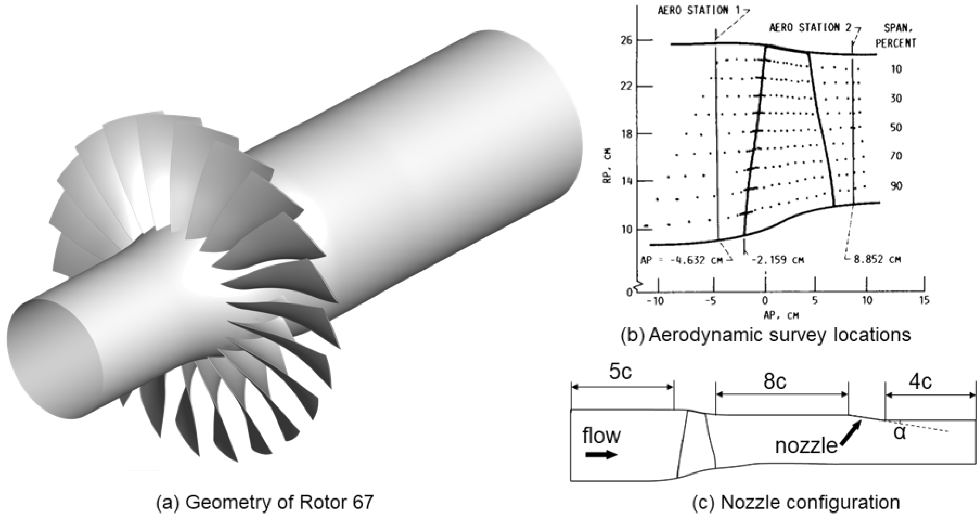
The geometric model used for the calculations is shown in Figure 1. The geometric model is represented in Figure 1a. The aerodynamic survey locations are marked in Figure 1b. Some specific settings in the computational domain are shown in Figure 1c. In Figure 1c, the distance between the leading edge of the blade and the inlet surface is 5 times the axial chord length of the blade. In order to simulate the flow field under near-stall conditions more accurately, some treatments are required, such as the exit nozzle referred to in some of the published research [19,20].
3.3. Calculation Model and Settings
The full-annulus structured grid used for the calculations in this paper is generated by AutoGrid5. The grid near the blade is constructed by the O4H-type topology. The tip difference is divided by using the butterfly grid to ensure the accuracy of the tip leakage flow calculation. y+ values are set to less than 5 to ensure the fineness of the grid near the blade surface.
Numerical calculations are carried out with the help of a commercial CFD code, NUMECA. The flow field solution is achieved by the finite volume method. For the spatial scheme, the second-order upwind Van Leer TVD limiter format is adopted. The double-time step method is used for the unsteady calculations. The turbulence model is Spalart-Allmaras (SA) model.
The boundary conditions given in the calculation are pressure, temperature, and velocity direction. The inlet total pressure and inlet total temperature are assigned with reference to the experimental conditions shown in Table 2. The outlet boundary is given as atmospheric pressure. Referring to Figure 1, the calculation starts from angle α = 0°. The complete performance map is obtained by increasing the angle α to reduce the opening of the nozzle. When both the conditions of mass conservation and residual stability are satisfied, the calculation is considered to be converged. The operating conditions are determined by nozzle opening, and the calculations under different conditions are carried out with intervals of 1% of the full opening. There are 22 blade channels in the full-flow channel. Each channel is observed with 20 timesteps, thus there are 440 time-steps in total in a revolution.
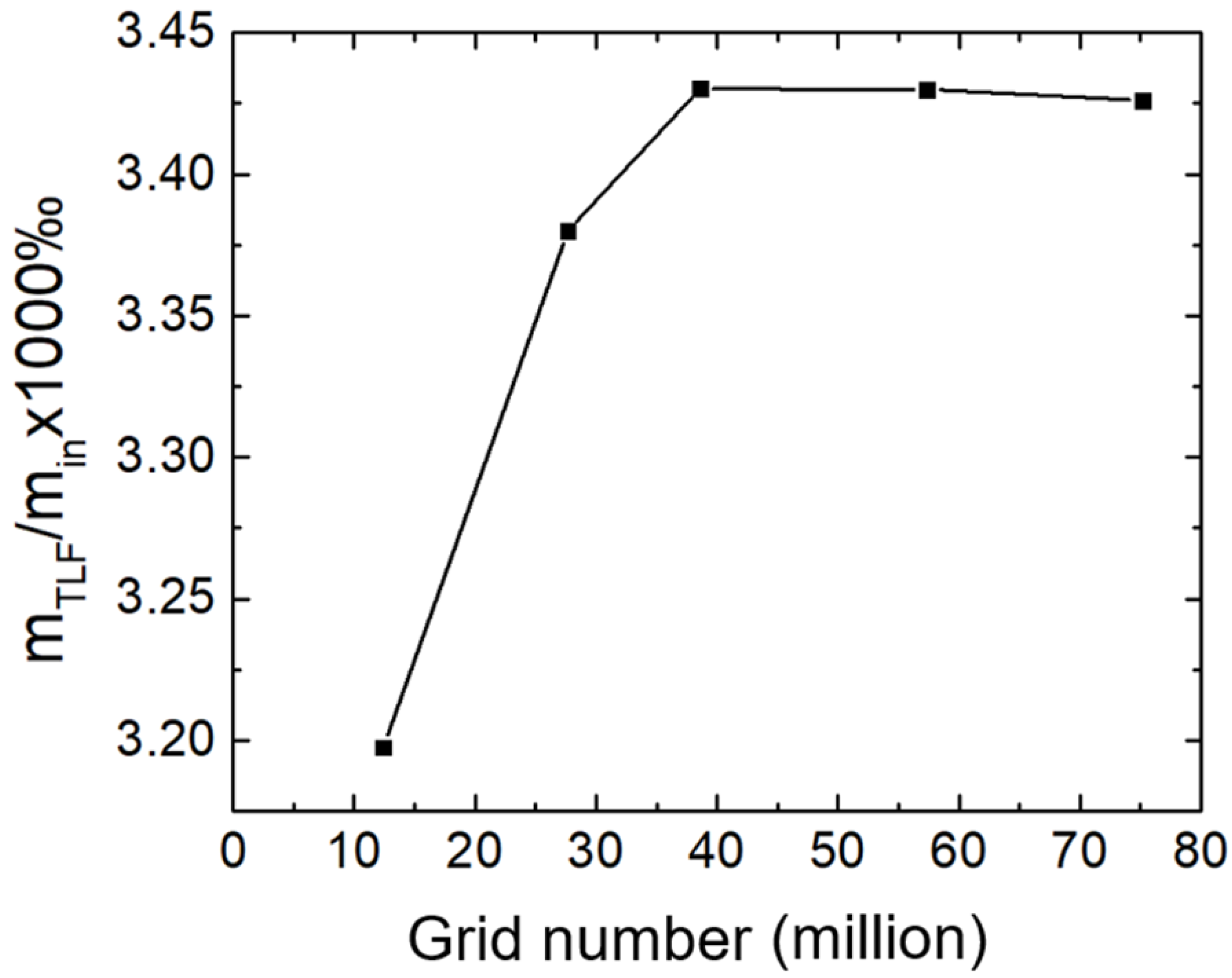
In order to study the grid independence, five sets of meshes as shown in Table 3 are evaluated.
The tip leakage mass flow rate, which has a significant impact on the accuracy of the results, is used as the criterion for the grid-independence verification. The grid-independence verification is completed under near-stall conditions. The results are shown in Figure 2. In this figure, the longitudinal axis is the dimensionless flow rate, which is the ratio of the tip leakage flow mass flow rate to the inlet mass flow rate (). It is found that the dimensionless flow rate is changed little from Grid 3 to Grid 4 and Grid 5. So, Grid 3 with a total grid size of 38.7 M is considered a suitable grid strategy.
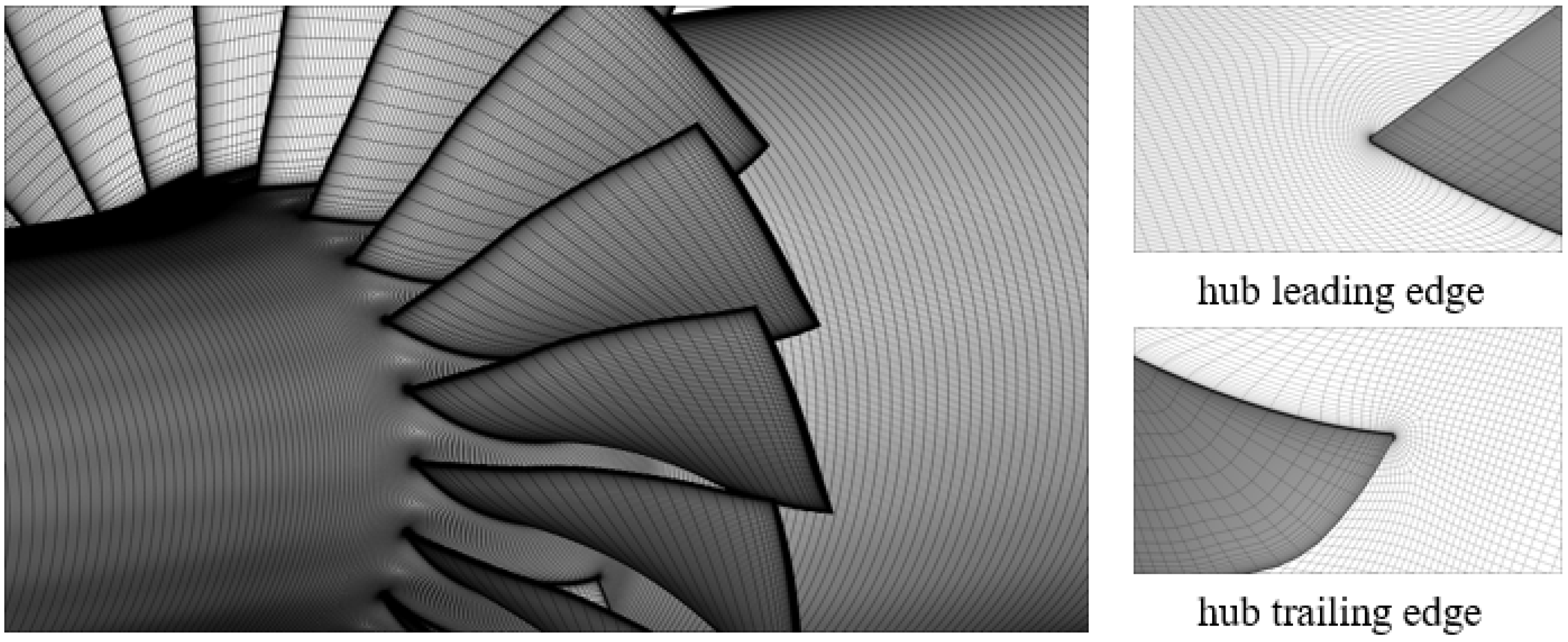
The grid detail is shown in Figure 3. The full-flow channel model is adopted in the unsteady calculation. Mesh around the leading edges, trailing edges and walls is well-refined in the grid-generating process.
3.4. Validation of Calculation Results
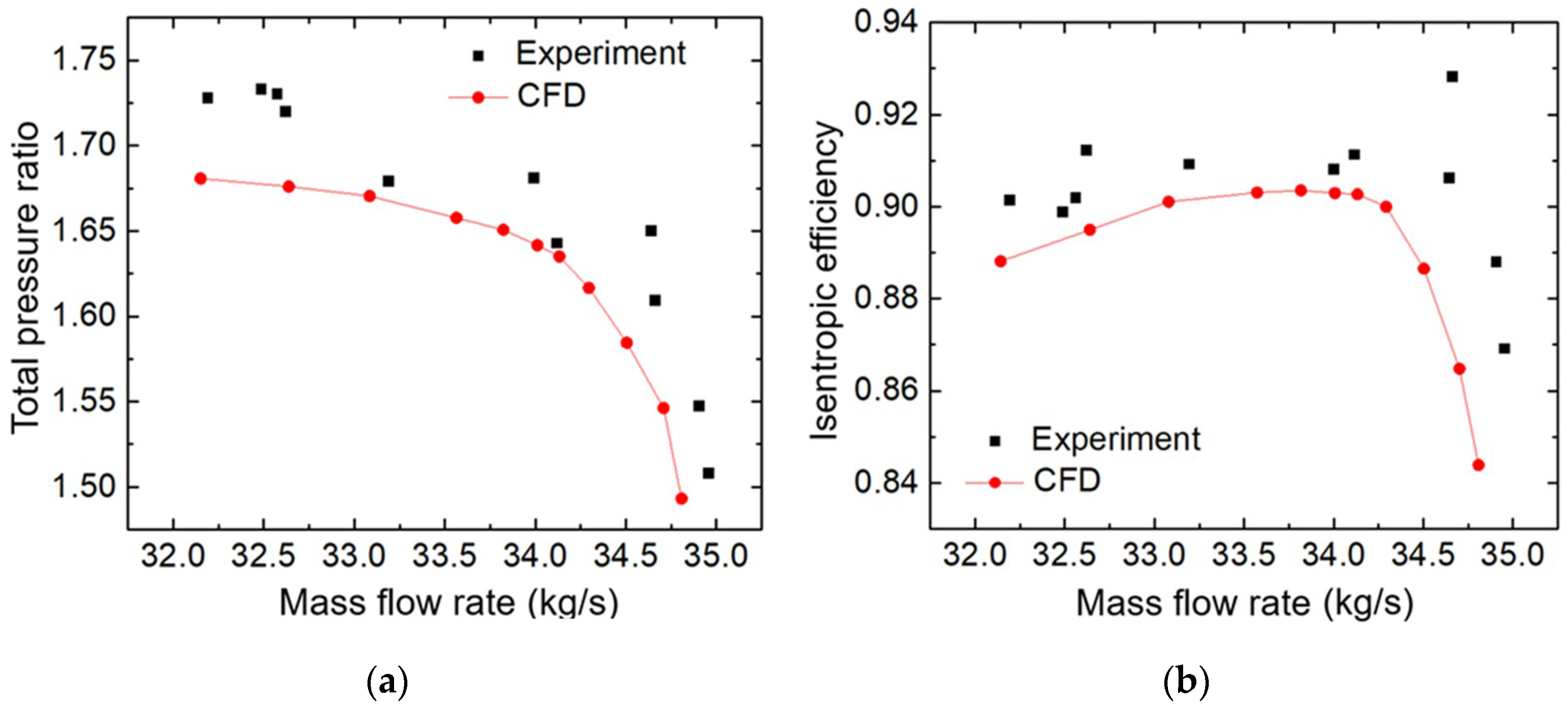
A comparison between the results from the numerical simulations and the experimental data [18] is presented in Figure 4. The time-average steady calculation results are used for comparison. It is found that the simulation results are in general consistent with the experimental data.
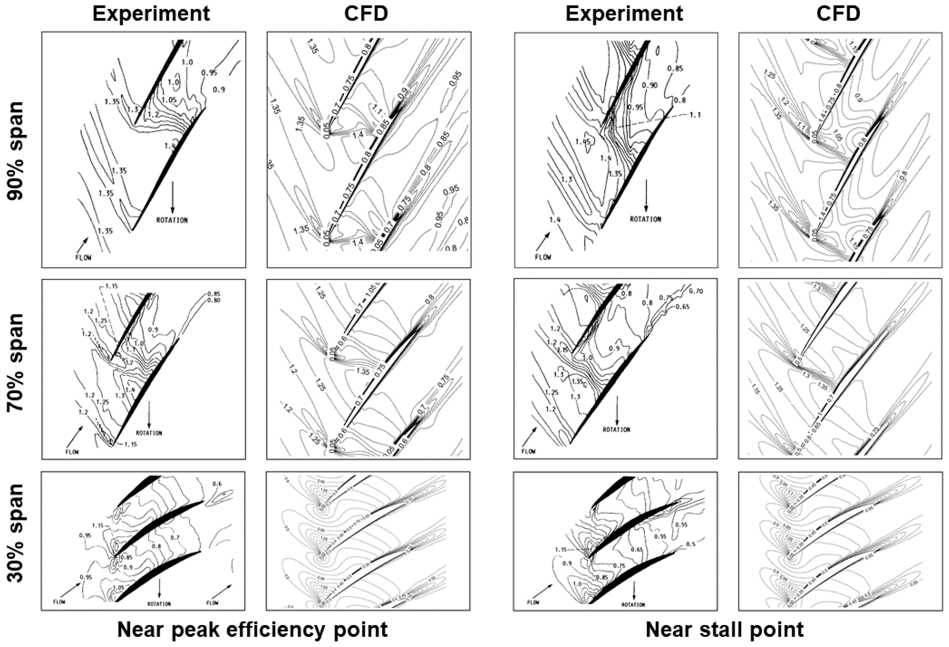
The isolines of relative Mach number at 90%, 70%, and 30% relative blade height under peak efficiency as well as near stall condition are shown in Figure 5. It can be observed that the simulation results are basically consistent with the experimental results. So, it is thought that the results obtained from the simulations are in general agreement with the experimental data and can be used for the following analysis.
3.5. Analysis of Unsteady Calculation Results
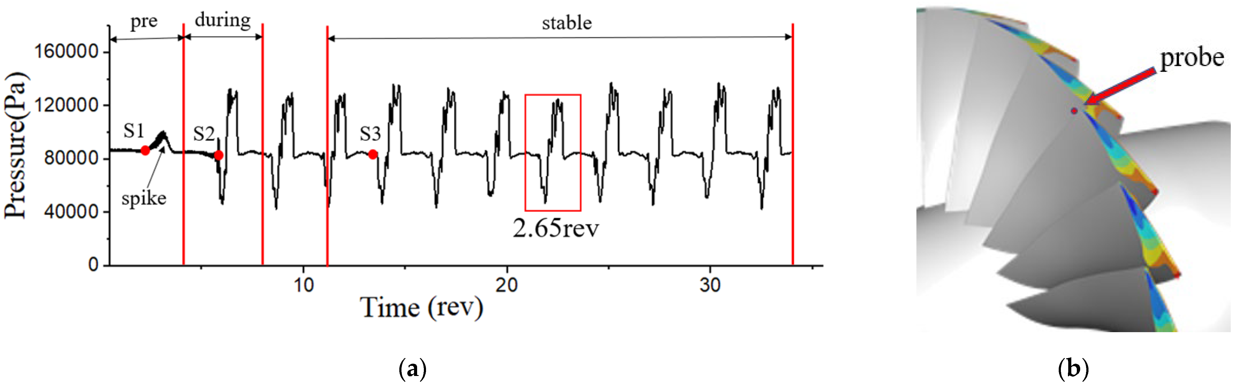
The unsteady flow characteristics of the stall process are illustrated in this part. The unsteady pressure probed in front of one of the blade’s leading edges is shown in Figure 6. Probe location is shown in Figure 6b. The pressure curve can be divided into three sections which respectively respond to three stall stages as mentioned before. They are labeled in the figure. Before the stall cells are formed, the disturbance in the pre-stall stage, which dominates the flow field, has the obvious features of high frequency with low amplitude and presents a spike-type appearance. When the disturbances are significantly strengthened in amplitude, the stall cell is generated and gradually developed, then the stall is in the during-stall stage. When the stable trough is found, it is considered that the stall is in the third stage of the stable-stall. As shown in the figure, the pressure in this stage is in a stable period after three revolutions of the stall cell. The period of the stall cell is about 2.65rev, which indicates the rotating speed of the stall cell is (2.65 − 1)/2.65 = 62.3% of the compressor rotating speed in the absolute frame.
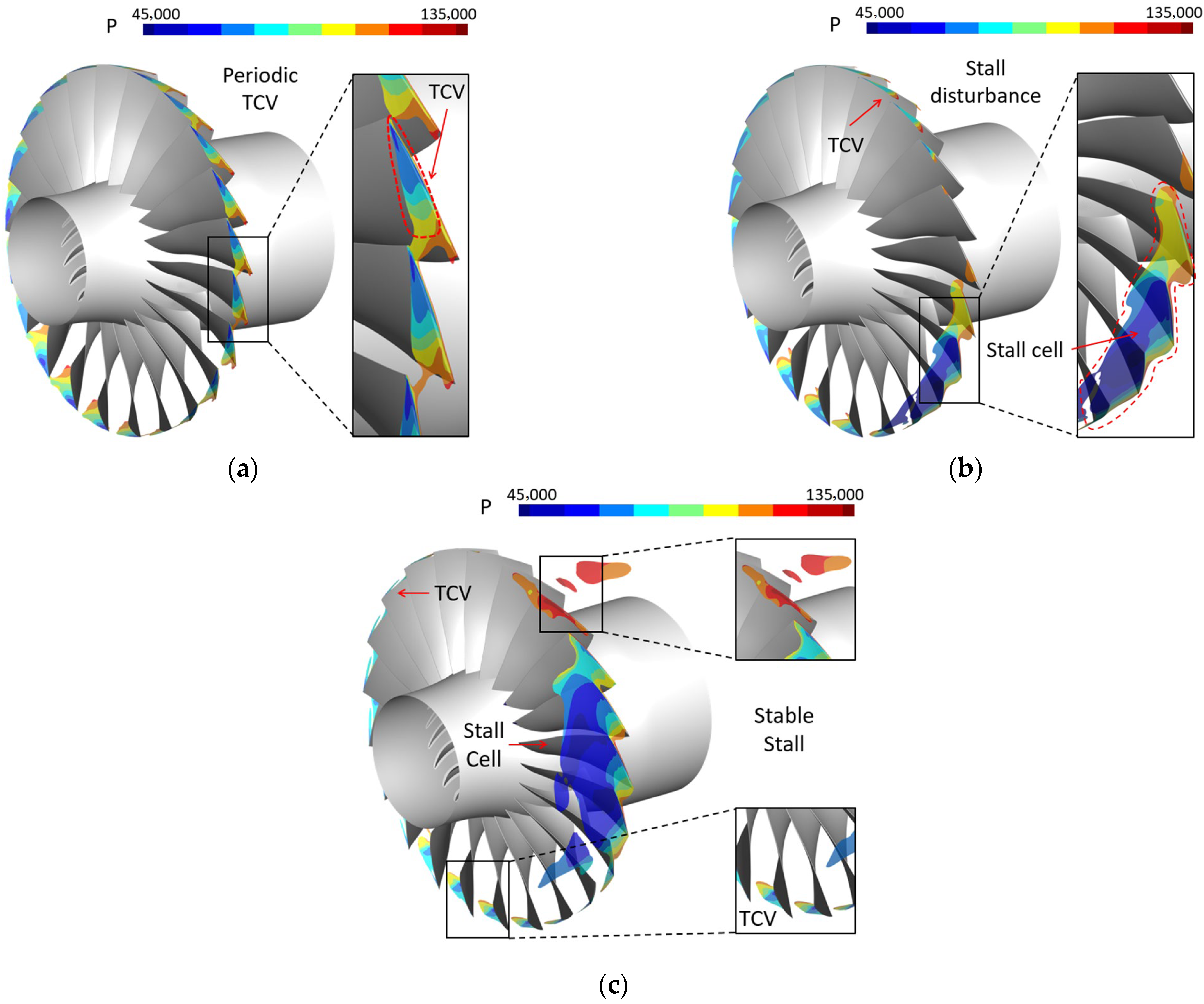
The detailed 3D unsteady flow fields at S1, S2, and S3 points labeled in Figure 6 are presented in Figure 7. Specifically, the vortex characteristic of the unsteady flow field is illustrated by the use of the iso-surface of the absolute value of the helicity. The helicity is defined as shown in Equation (10).
In Figure 7, it is only in the tip region where the absolute value of helicity is very high due to the leakage flow, especially at the leading edge of each blade. Thus, the flow field around the blade’s leading edge is strongly influenced by the tip leakage flow and has special flow features, which can be used to describe the stall. As the flow field near the blade tip has the most significant effect on the whole flow field, the analysis of the flow characteristics at the span of 99% can be used to understand the whole flow field somewhat. At point S1, the stall is in the pre-stall stage before the stall cell occurs, and the TCVs in the tip region have the same flow characteristics in the circumferential direction. Then, at point S2, the stall cells have been formed, and some cells are grouped so that the low-pressure area upstream of the leading edge under the influence of the group is very extensive. It is due to the stall cell group that the channels are blocked and mass flow in these blocked channels is decreased obviously. All the same, the blocked mass flow is pushed into the neighbor channels and the flow state in these channels is improved accordingly. So, it is found in the figure that the helicity of the region close to the stall cell group is low relatively, even lower than that in the pre-stall stage. However, at point S3, the group is grown up and the stall is in the stable-stage. In the stage, the difference between the region influenced by the group and the left region is very distinctive so the high helicity cannot be found except for the influenced region.
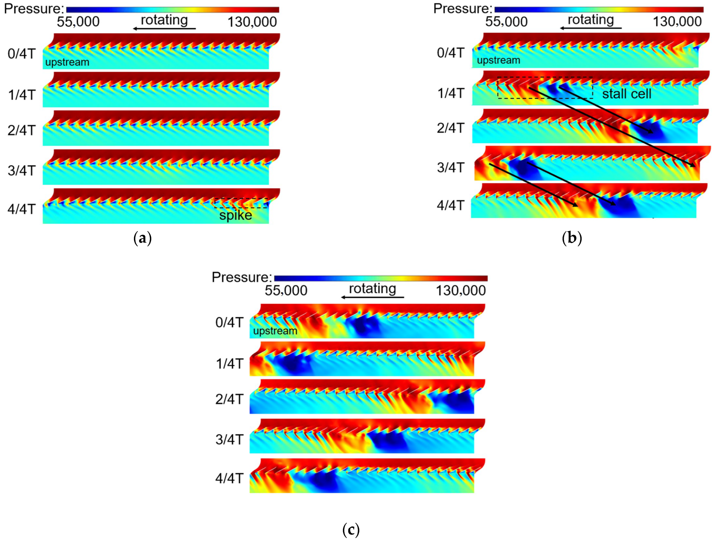
The unsteady pressure distribution of the three stages at a span of 99% is shown in Figure 8. In this figure, T is the consumption time of calculation for each stage respectively. In the pre-stall stage in Figure 8a, the main features of the flow field are determined by the mean flow field, while the parameters pulsation is dominated by high-frequency disturbances. In the beginning, as some stall characteristics have not appeared yet, the flow field now seems to be circumferential uniform. However, during the second half of time, the spike-type disturbances with the high-amplitude and the low-frequency can be found in the pulsation. The formation process of the stall cells is shown in Figure 8b. The first stall cell with obvious circumferential distribution features, low frequency, and high amplitude, appears and is gradually developed until it becomes stabilized. Then, the stall is in the stable-stage with a stable rotating speed, as shown in Figure 8c.
4. Research Model and Numerical Setup
In this section, the distribution of total pressure is used in the calculation of POD. The modal decomposition results with several orders are validated by comparing them with the original flow field. It is because the features of the stall cells are critical and important for the whole analysis that the stable-stall stage is analyzed first. Thereafter, the analysis is focused on the generating and developing process of the stall cells. Meanwhile, the capability of reducing data dimension for the POD method is also evaluated in three stall stages.
4.1. Validation of Modal Decomposition Results
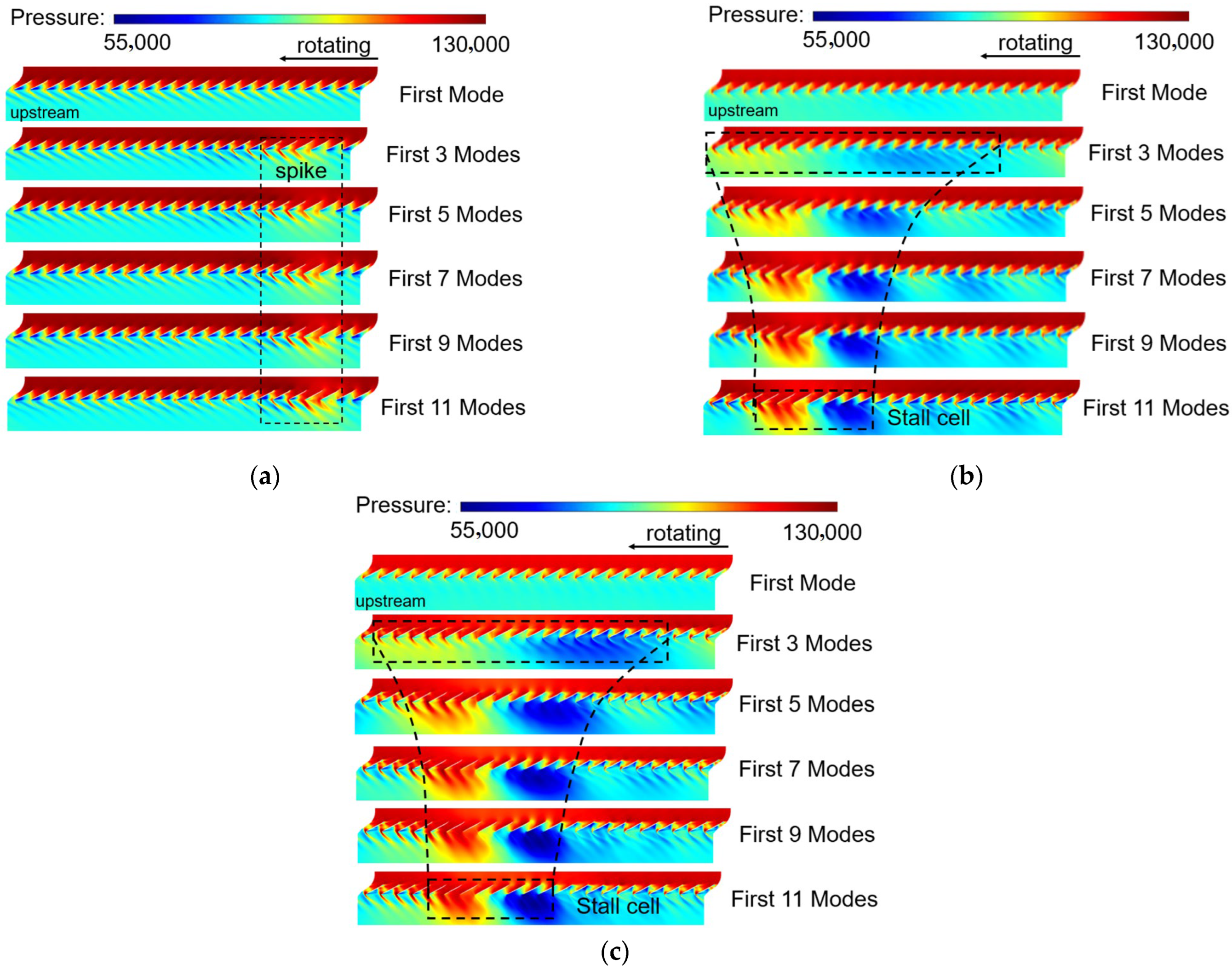
Different POD reconstruction results of three stall stages calculated by Equation (6) are shown in Figure 9. In order to make the comparison between the decomposition results and the original flow field more easily, the snapshots with the most prominent characteristics have been selected, such as the moment 4/4T for the pre-stall stage, 1/4T for the during-stall stage and 0/4T for the stable-stall stage respectively. It is found from the figures that the stall cell features in Figure 9b,c is particularly obvious. When the order of flow field reconstruction is increased, the decomposition results are close to those of the original flow field more and more. When the order of POD modes involved in the reconstruction reaches 11 or more, the reconstruction results do not change significantly with the increasing order. Therefore, the results of the 11th reconstruction are adopted in the following words to analyze the low-order POD reconstruction in this paper.
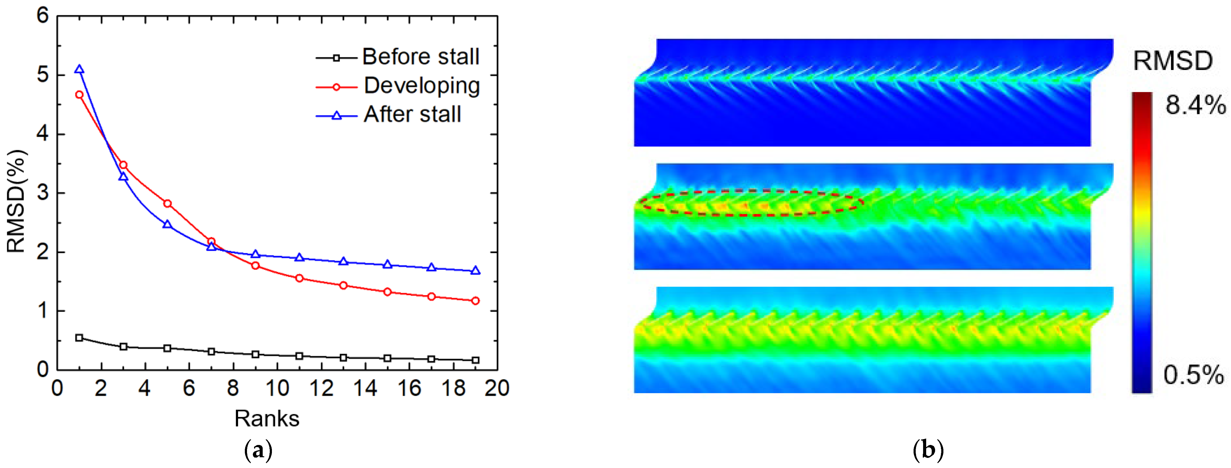
In this paper, the root-mean-square deviation (RMSD) is used to evaluate the POD reconstruction results at each grid point. Actually, the RMSD is the error between the reconstructed results and original unsteady values over the full-time range. For each point in the flow field, the RMSD is calculated as the following.
where n is the total number of computational time steps, the value of the low-rank reconstruction result, and the solution of the unsteady calculation. In this paper, the RMSD is normalized by the inlet total pressure.
The overall RMSD is determined by means of the geometric mean over the full flow field. The overall RMSD is shown in Figure 10a. It is observed that the overall RMSD is gradually decreased with the order increasing until to 11th order. When the order is increased to 11th or more, the overall RMSD of the pre-stall stage is less than 0.5%, while those of the left two stages are higher a little, but less than 2%. In frank, the POD method is more suitable for the processing of signals with high frequency. When the stall cells with low frequency are formed and become stable more and more in the during-stall stage and the stable-stall stage, the frequency of the whole unsteady flow field is decreased accordingly so that the error of the reconstruction results is affected negatively. The RMSD distribution is shown in Figure 10b. In the pre-stall stage, it is in the region from the upstream of the leading edge to the middle of the blade that the RMSD is high. In contrast, the regions with high RMSD are extended downstream of the outlet of the flow channel for the during-stall stage and the stable-stall stage as well as the RMSD value is increased obviously. It is very interesting that the maximum RMSD is found upstream of the leading edge of nine flow channels in the during-stall stage. In our experience, the accuracy of the POD method is affected by the periodicity of the original flow field and low periodicity would bring about low accuracy of the reconstruction results. So, it is due to the obvious circumferential heterogeneity of the original flow parameters in these nine flow channels that gives rise to the higher RMSD during the development of the stall cells.
4.2. Analysis of POD Results on the Stable-Stall Stage
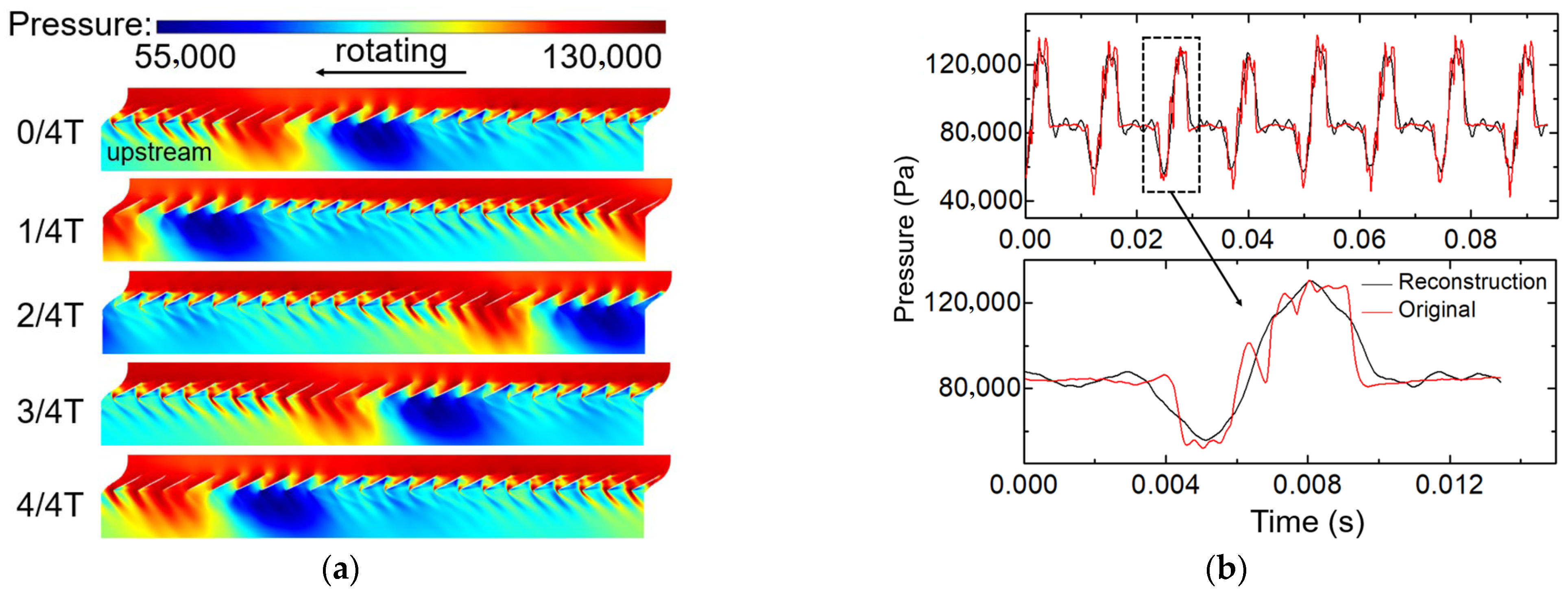
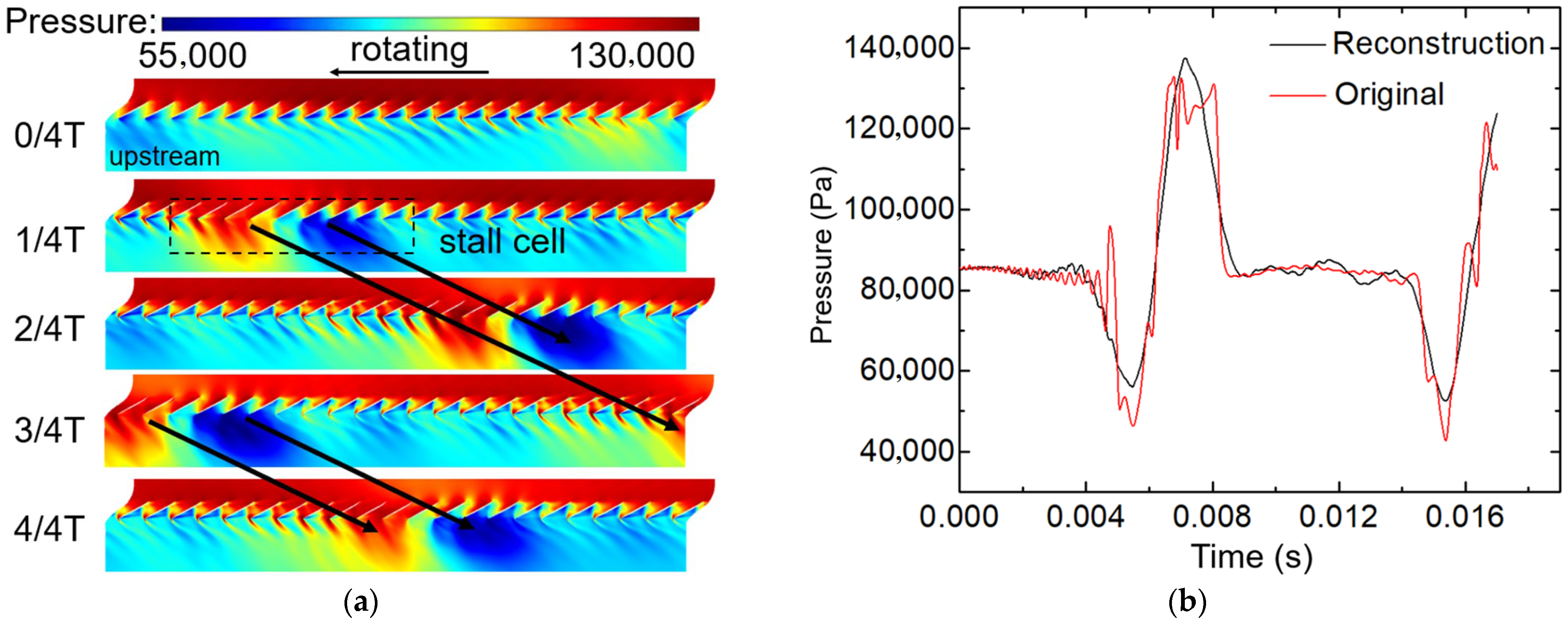
In Figure 11a, the reconstructed unsteady flow field by 11 modes is shown over the time duration which is consistent with that of the original flow field shown in Figure 8c. The main characteristics of the stall cells are well captured. A quantitative comparison of the pressure distribution between the original flow field and the reconstructed flow field at the probe in front of the tip leading edge is shown in Figure 11b. The difference between the two distributions is so small that the reconstructed results can be considered satisfactory results. In detail, the low-frequency perturbation caused by the stall cells is perfectly captured, while the high-frequency perturbation is missed by the neglecting of other higher modes.
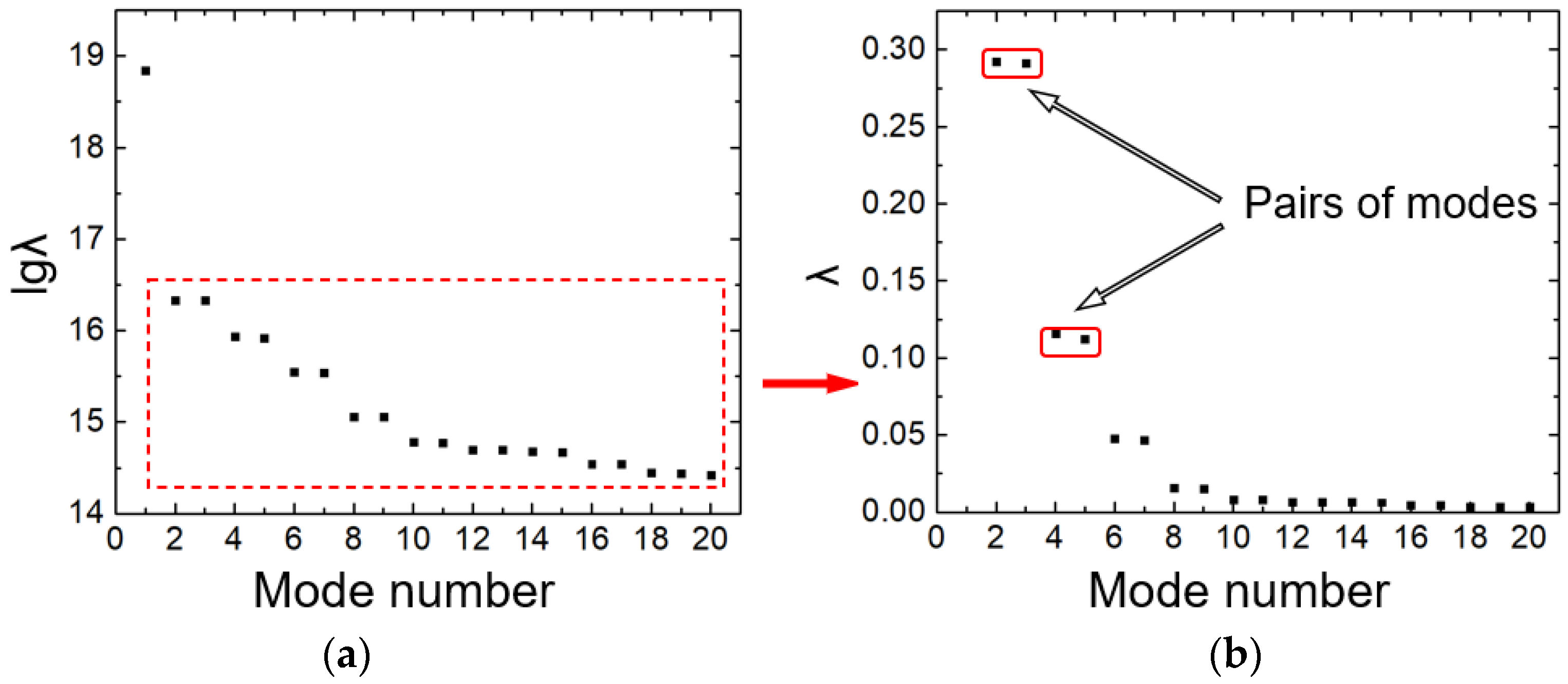
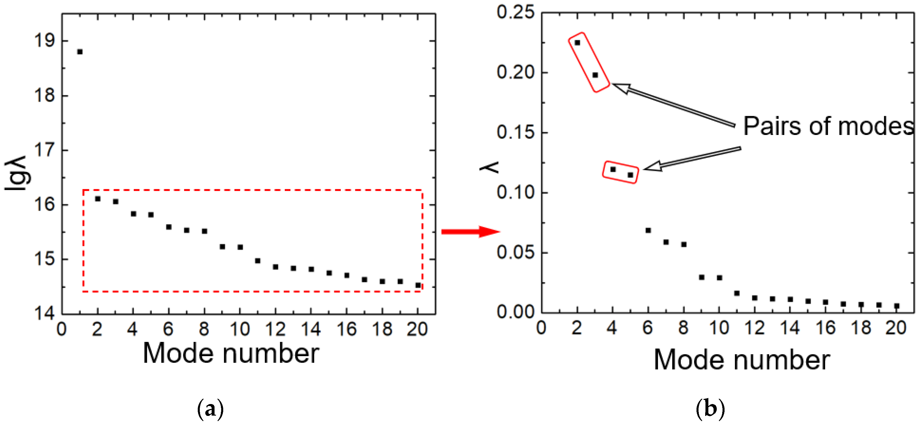
The POD mode eigenvalues calculated by Equation (3) are illustrated in Figure 12. The eigenvalues of all the modes are extracted from the stable stall flow field as shown in Figure 8c. Except for the mean-flow mode (mode 1), the eigenvalues of the other modes are always in pairs. The energy seems to be the same to each other in every pair. Mode 1 is related to the averaged flow characteristics so it is excluded from the following analysis in order to focus on the characteristics related to the stall. In Figure 12b, the eigenvalues of the stall cell modes except mode 1 are shown. Furthermore, the eigenvalues in this figure are normalized by the sum of all eigenvalues. It is found that the energy of the first two eigenvalue pairs, the pair of modes 2 and 3 and the pair of modes 4 and 5, is changed sharply. However, about 80.3% of the stall cell energy is occupied by these modes. Thus, the main characteristics of the flow field pulsation can be described by these modes. The other subordinary modes can be adopted to analyze more details of the stable-stall stage.
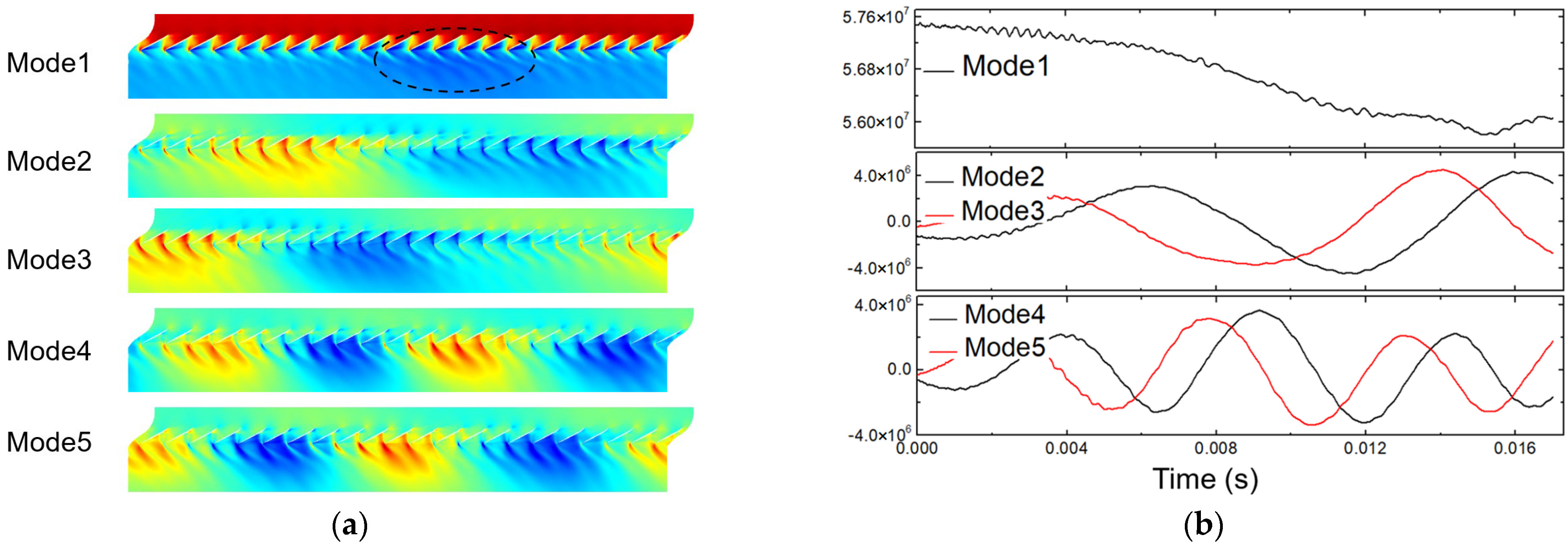
In Figure 13, the mode and the mode coefficient of the first five modes calculated by Equations (4) and (5) are presented. The horizontal axis of Figure 13b is the time step same as the axis of Figure 11b. From the mode contours, it can be recognized that mode 1, mode 2–3, and mode 4–5 are the mean flow mode, the SRF mode, and the harmonic mode of the SRF mode, respectively. It is found the description of the stall cell structure in the flow field by the POD mode is similar to that by the Fourier transform, by which a series of modes with harmonic periodic fluctuation in space and time are established. Meanwhile, as labeled in Figure 8, the stall cell wave speed of SRF mode, which is the product of the wavelength in space and frequency in time, is Aω, while the stall cell wave speed of its harmonic mode is A/2 × 2ω = Aω. It indicates that no matter how many orders are considered, their wave speeds are in the same value although their mode wavelength and the mode frequency are different from each other.
Mode 1 differs from the other modes because it reflects the mean-flow characteristics. As shown in Figure 12a, when the mode is taken into account in the energy spectrum, it occupies most part of the mode energy. The spatial distribution of the parameters in each flow channel is the same in the circumferential direction. Furthermore, unlike the time coefficient curves of the other modes which are basically similar to the sinusoidal curve, there are complex frequency components in the time coefficient of mode 1.
As the flowing becomes stable, the characteristics of every mode except mode 1 are periodic along the circumferential direction, so a spatial distribution decomposed from the results of the full flow channel at any moment can be obtained through the investigation of the parameter distribution of a single channel over a period. However, the frequencies of different pairs are different. It is also found in this figure that the features of the leading-edge shock are more prominent due to the circumferential rotational disturbance. It indicates the leading-edge shock is sensitive to the rotational disturbance, but at present, the relationship between the leading-edge shock and the rotational disturbance is not very clear. In this paper, with the help of the POD method, the relationship can be understood deeply. This is one of the advantages of the POD method compared with directly analyzing the original flow field. The shock is triggered at the leading edge, developed into a flow channel, and acted on the next blade suction surface at the last. Based on the above analysis, it is near the region around the leading edge that the helicity of the leakage flow is very strong so that the leakage flow has a deep relationship with the leading-edge shock. The closer to the leading edge, the more significant the influence is. This is why the shock wave is called a leading-edge shock wave.
4.3. Analysis of POD Results on the Pre-Stall Stage
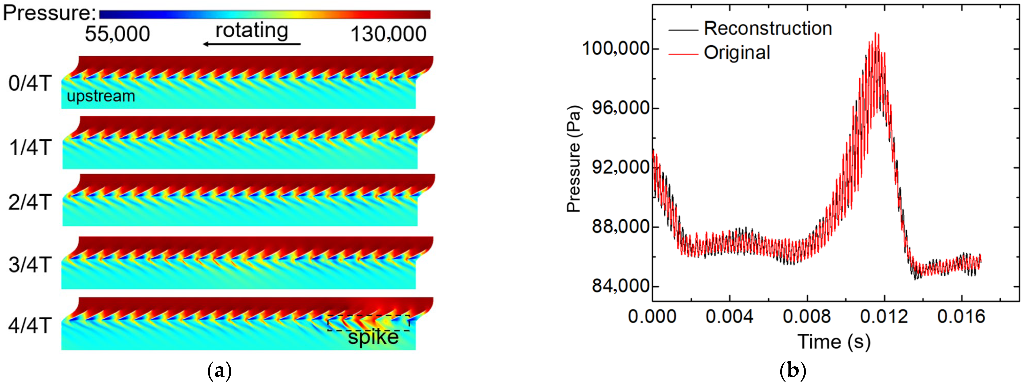
The results of the reconstructed flow field in the pre-stall stage are presented in Figure 14. The reconstructed unsteady flow field is shown in Figure 14a, and the time duration is consistent with that of the original flow field in Figure 8a. The spike-type disturbance is well captured, which is almost the same as that found in the original flow field. A quantitative comparison of the pressure curves between the original flow field and the reconstructed flow field at a point on the leading edge of the blade is shown in Figure 14b. The error between the two curves is small. Furthermore, it is smaller than that in the stable-stall stage because the 1BPF component dominates the pre-stall flow field and the periodic abrupt waves brought by the stall cells have not been found yet. So, it can be concluded that the reconstruction accuracy based on the first 11 modes is sufficient for the following analysis.
The characteristics of the POD mode eigenvalue calculated by Equation (3) in the pre-stall stage are illustrated in Figure 15. The energy proportion of mode 1 related to the mean flow is greater than that of mode 1 in the stable-stall stage because the spike-type disturbance in the pre-stall stage is weaker than that in the stable-stall stage. The eigenvalues except for the mean flow field (mode 1) are shown in Figure 15b. Although the energy proportion of the two neighbored modes is different, the two modes are still considered to be in a pair referred to as the mode characteristics presented in Figure 16a.
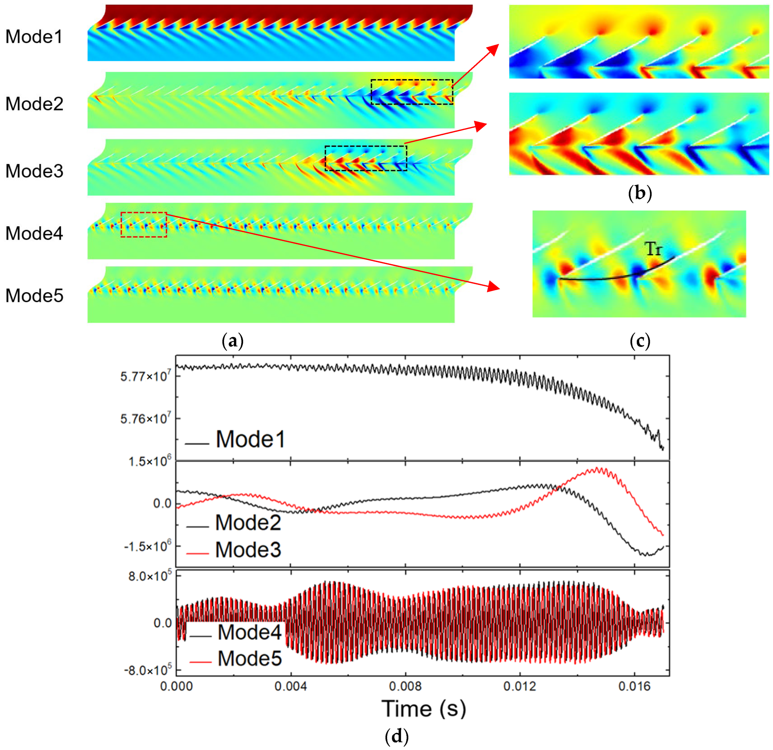
In Figure 16, the parameter distributions and the time coefficient of the first 5 modes calculated by Equations (4) and (5) are presented. As analyzed before, the stall cell has not yet formed, and the spike-type disturbance can be found in the parameter distributions. Therefore, in Figure 16a,d, this kind of disturbance is observed in several flow channels, which are gradually developing with time. At the same time, negative values compared to the disturbance appear downstream of the trailing edge, zoomed in Figure 16a mode 2 and mode 3. Combined with the original flow field in Figure 8a, this phenomenon can be seen as the characteristic of the reverse flow vortex, which is the inception of the stall cell before its full development and is not presented in the stable-stall stage. So, it is convinced that some information related to the stall can be effectively extracted by the POD method even if the stall is in the inception stage.
Unlike the POD results of the stable-stall stage, the TCV breaking process can be investigated by the POD results of mode 4 and mode 5 in the pre-stall stage, zoomed out in Figure 16c. The TCV moves along the Tr line from the leading edge of the first blade to the pressure side of the neighboring blade. It is presented with a vortex feature, with positive and negative values alternatively. Before the stall cells occur, the induced velocity of the leakage vortex is balanced by the component of the main flow normal to the vortex, so that the TCV trace is stabilized at a position near the leading edge and almost perpendicular to the mainstream until TCV is adsorbed on the pressure surface of the next blade. It is found in Figure 16d that at the end of the time the stall cell gradually occurs and the pre-stall feature, TCV, gradually decayed in the amplitude of the time coefficients.
From the analysis of mode 2 and mode 3, the POD method can extract the unobvious feature of the reverse flow vortex downstream of the trailing edge from the original flow field. Thus prove the dependency of this feature and the spike-type disturbance. This ability is also shown in mode 4 and mode 5. The TCV, which is almost indistinguishable from the original flow field, can be decomposed into these modes. Compared with the method of direct analysis, the POD method effectively improves the ability to capture and analyze the unobvious flow features.
4.4. Analysis of POD Results on the During-Stall Stage
In Figure 17, the reconstruction result of the flow field is presented. Compared with the stall cells in the stale stage, similar stall cells also can be found, but their periodicity is not obvious in this stage.
The characteristics of the POD mode eigenvalue calculated by Equation (3) in the during-stall stage are illustrated in Figure 18. The parameter distribution and the time coefficient of the first 5 modes are presented in Figure 18. From these two figures, it is considered that the configuration of two neighbored modes except mode1 is still in a pair, just as in the pre-stall stage, but their energy levels are different from each other. The energy difference between the two paired modes is less than that in the pre-stall stage but much larger than that in the stable-stall stage. So, it is reasonable to treat the during-stall stage as a kind of transition process, in which the eigenvalues of the paired modes have gradually approached each other until they reach an equal level and then into the stable-stall stage finally.
As analyzed before, the stall cell is formed but not stable. The modes related to the tip leakage flow in the pre-stall stage have disappeared while the modes are replaced by the characteristic modes related to the stall cell and its harmonic multiples. It is shown in Figure 19 that the mean flow referred to as mode 1 becomes more unstable due to the unstable features of the stall cells in this stage. At the end of the stage, there is an obvious increase in amplitude for mode 2 and mode 3. It indicts that the stall cells are gradually developed to a higher level and begin to influence the flow field greatly.
5. Discussion
From the analysis above, the evolution of the stalled process is studied by the means of proper orthogonal decomposition (POD) method in detail. However, there are still limitations on the deeper usage of the POD on the rotating stall.
Firstly, the POD method is designed based on the periodic process. The stalled process needs to be divided into different stages to make sure the POD results can be considered as a separate periodic process. Although in this paper the division works well, this method still needs to be improved for further study.
Secondly, the POD method has a limited ability to deal with low-frequency information on flow characteristics. For data dominated by low-frequency information, the amount of data required will increase significantly. In recent years, spectral proper orthogonal decomposition (SPOD) appears [24], which is expected to solve this problem.
6. Conclusions
In this paper, the evolution of the stalled process and flow characteristics of the flow field structure are analyzed by the use of the POD method. NACA Rotor 67 is adopted as a model and three-dimensional unsteady calculation is used to provide the material for POD. It shows that the POD method is an effective method for the analysis of rotating stall flow. The conclusions of this paper are summarized as follows.
- (1)
- The POD method has the ability to decompose flow characteristics into different POD modes based on their influence on the flow field. Compared with the method of analyzing the original unsteady flow field of the rotating stall process, the POD result is more direct and accurate.
- (2)
- The reconstruction of the POD results is satisfactory. With the increase of the reconstruction order, the reconstruction error according to RMSD judgment is gradually decreased. The reconstruction based on the 11 modes is accurate as its average error is below 2%, which is accurate enough for the analysis of the rotating stall process.
- (3)
- From POD results in the stable-stall stage, the eigenvalues of modes except for the mean-flow mode (mode 1), are always in pairs with similar frequency and energy proportion. The modes of the periodically stable stall cell decomposed by the POD method exhibit sinusoidal characteristics similar to those by the Fourier transform in time and space. At the same time, it is found that the stable stall cells can give rise to a rotational disturbance at the leading edge, which can trigger the shock wave over there. When the leading-edge shock wave is formed, it is developed into a flow channel and acted on the next blade suction surface at the last.
- (4)
- In the pre-stall stage, based on the analysis of mode 2 and mode 3, the features of the reverse flow vortex downstream of the trailing edge can be extracted by the POD method from the original numerical results. It is proved that the development of the reverse flow vortex can attribute to the spike-type disturbance. Furthermore, the TCV can also be identified by mode 4 and mode 5, which can be treated as the precursor of stall during the early process in this stage.
- (5)
- It is revealed by the analysis of the POD results that in the during-stall stage, the stall cells are gradually developed with sinusoidal characteristics, while the effect of the leakage flow is decayed and can not be found in the low-order modes. Although in this stage the flow field is with strong non-linearity, the POD method is still capable of handling and decomposing it successfully.
Author Contributions
Methodology, Y.W. and M.S.; software, Y.W.; validation, Y.W.; formal analysis, Y.W.; investigation, Y.W.; resources, B.Y.; data curation, M.S. and J.X.; writing—original draft preparation, Y.W.; writing—review and editing, M.S. and B.Y.; project administration, M.S.; funding acquisition, B.Y. All authors have read and agreed to the published version of the manuscript.
Funding
This work was supported by National Science and Technology Major Project (2017-II-0006-0019).
Institutional Review Board Statement
Not applicable.
Informed Consent Statement
Not applicable.
Data Availability Statement
Not applicable.
Acknowledgments
This work was supported by National Science and Technology Major Project (2017-II-0006-0019). This support is gratefully acknowledged.
Conflicts of Interest
The authors declare no conflict of interest.
References
- Johnsen, I.A.; Bullock, R.O. Aerodynamic Design of Axial-Flow Compressors; NASA SP-36; Scientific and Technical Information Division: Cleveland, OH, USA, 1965. [Google Scholar]
- Day, I.J. Stall, Surge, and 75 Years of Research. J. Turbomach. 2016, 138, 011001.1–011001.16. [Google Scholar] [CrossRef]
- Schlechtriem, S.; Tzerich, M.L. Breakdown of Tip Leakage Vortices in Compressors at Flow Conditions Close to Stall; ASME: Orlando, FL, USA, 1997. [Google Scholar]
- Adamczyk, J.J.; Celestina, M.L.; Greitzer, E.M. The role of tip clearance in high-speed fan stall. J. Turbomach. 1993, 115, 28–38. [Google Scholar] [CrossRef]
- Yamada, K.; Furukawa, M.; Inoue, M.; Funazaki, K.I. Numerical analysis of tip leakage flow field in a transonic axial compressor rotor. In Proceedings of the International Gas Turbine Congress; Academic Press: Tokyo, Japan, 2003; pp. 1–8. [Google Scholar]
- Pullan, G.; Young, A.M.; Day, I.J.; Greitzer, E.M.; Spakovszky, Z.S. Origins and Structure of Spike-Type Rotating Stall. J. Turbomach. 2015, 137, 051007.1–051007.11. [Google Scholar] [CrossRef]
- Day, I.J. Stall inception in axial flow compressors. Turbo Expo: Power for Land, Sea, and Air. Am. Soc. Mech. Eng. 1991, 78989, V001T01A034. [Google Scholar]
- Camp, T.R.; Day, I.J. A study of spike and modal stall phenomena in a low-speed axial compressor. J. Turbomach. 1998, 120, 393–401. [Google Scholar] [CrossRef]
- Hah, C.; Bergner, J.; Schiffer, H.P. Short length-scale rotating stall inception in a transonic axial compressor: Criteria and mechanisms. Turbo Expo Power Land Sea Air 2006, 4241, 61–70. [Google Scholar]
- Melius, M.; Cal, R.B.; Mulleners, K. POD based analysis of three-dimensional stall over a pitching wind turbine blade. 68th Annual Meeting of the APS Division of Fluid Dynamics. Am. Phys. Soc. 2015, D28, 006. [Google Scholar]
- Lumley, J.L. The structure of inhomogeneous turbulent flows. In Atmospheric Turbulence and Radio Wave Propagation; Nauka: Moscow, Russia, 1967; pp. 166–178. [Google Scholar]
- Sirovich, L. Turbulence and the dynamics of coherent structures. III. Dynamics and scaling. Q. Appl. Math. 1987, 45, 583–590. [Google Scholar] [CrossRef] [Green Version]
- Aubry, N.; Holmes, P.; Lumley, J.L.; Stone, E. The dynamics of coherent structures in the wall region of a turbulent boundary layer. J. Fluid Mech. 1988, 192, 115–173. [Google Scholar] [CrossRef]
- Ma, X.; Karniadakis, G.E. A low-dimensional model for simulating three-dimensional cylinder flow. J. Fluid Mech. 2002, 458, 181–190. [Google Scholar] [CrossRef] [Green Version]
- Wu, Y.; Lee, H.M.; Tang, H. A study of the energetic turbulence structures during stall delay. Int. J. Heat Fluid Flow 2015, 54, 183–195. [Google Scholar] [CrossRef]
- Mallik, W.; Raveh, D.E. Aerodynamic damping investigations of light dynamic stall on a pitching airfoil via modal analysis. J. Fluids Struct. 2020, 98, 103–111. [Google Scholar] [CrossRef]
- Sun, C.; Shi, L.; Shen, X.; Xiaocheng, Z.; Zhaohui, D. Analysis of POD for the Flow Field of the Wind Turbine Airfoil at High Angle of Attack. J. Eng. Phys. 2021, 42, 894–904. [Google Scholar]
- Strazisar, A.J.; Wood, J.R.; Hathaway, M.D.; Suder, K.L. Laser Anemometer Measurements in a Transonic Axial-Flow Fan Rotor; NASA TP 2879; Lewis Research Center: Cleveland, OH, USA, 1989. [Google Scholar]
- Vahdati, M.; Sayma, A.I.; Freeman, C.; Imregun, M. On the use of atmospheric boundary conditions for axial-flow compressor stall simulations. J. Turbomach. 2005, 127, 349–351. [Google Scholar] [CrossRef]
- Choi, M.; Vahdati, M. Numerical strategies for capturing rotating stall in fan. Proc. Inst. Mech. Eng. Part A J. Power Energy 2011, 225, 655–664. [Google Scholar] [CrossRef]
- Song, M.; Yang, B.; Zhu, G.; Tong, S.J.; Zhang, S.; Xie, H. Analysis on The Spike-type Rotating Stall for Axial Compressor by Dynamic Mode Decomposition. In Proceedings of the GPPS Conference, Xi’an, China, 18–20 October 2021. [Google Scholar]
- Khaleghi, H. Stall inception and control in a transonic fan, part A: Rotating stall inception. Aerosp. Sci. Technol. 2015, 41, 250–258. [Google Scholar] [CrossRef]
- Zhang, W.; Vahdati, M. Stall and recovery process of a transonic fan with and without inlet distortion. J. Turbomach. 2020, 142, 011003. [Google Scholar] [CrossRef]
- Karami, S.; Soria, J. Analysis of Coherent Structures in an Under-Expanded Supersonic Impinging Jet Using Spectral Proper Orthogonal Decomposition (SPOD). Aerospace 2018, 5, 73. [Google Scholar] [CrossRef]
Figure 1.
Geometric model of Rotor67.

Figure 2.
Grid-independence verification.

Figure 3.
Sketch of Grid 3.

Figure 4.
Comparison of performance curves. (a) Total pressure ratio. (b) Isentropic efficiency.

Figure 5.
Comparison of relative Mach number distribution at different blade heights.

Figure 6.
Pressure of a probe in front of the tip leading edge. (a) Pressure at probe. (b) Probe location.
Figure 6.
Pressure of a probe in front of the tip leading edge. (a) Pressure at probe. (b) Probe location.

Figure 7.
Three-dimensional unsteady vortex features. (a) Vortex characteristics of S1 (absolute value of helicity = 30,000). (b) Vortex characteristics of S2 (absolute value of helicity = 30,000). (c) Vortex characteristics of S3 (absolute value of helicity = 30,000).
Figure 7.
Three-dimensional unsteady vortex features. (a) Vortex characteristics of S1 (absolute value of helicity = 30,000). (b) Vortex characteristics of S2 (absolute value of helicity = 30,000). (c) Vortex characteristics of S3 (absolute value of helicity = 30,000).

Figure 8.
Original flow field. (a) Pre-stall flow field. (b) During-Stall flow field. (c) Stable-stall flow field.
Figure 8.
Original flow field. (a) Pre-stall flow field. (b) During-Stall flow field. (c) Stable-stall flow field.

Figure 9.
Reconstruction results. (a) Pre-stall stage reconstruction. (b) During-stall stage reconstruction. (c) Stable-stall stage reconstruction.
Figure 9.
Reconstruction results. (a) Pre-stall stage reconstruction. (b) During-stall stage reconstruction. (c) Stable-stall stage reconstruction.

Figure 10.
Comparison of reconstruction errors at different stages. (a) Variation of RMSD with reconfiguration rank. (b) Spatial distribution of RMSD.
Figure 10.
Comparison of reconstruction errors at different stages. (a) Variation of RMSD with reconfiguration rank. (b) Spatial distribution of RMSD.

Figure 11.
Flow field reconstruction results. (a) First 11 modes reconstruction flow field. (b) Pressure collected by the probe in front of the tip leading edge.
Figure 11.
Flow field reconstruction results. (a) First 11 modes reconstruction flow field. (b) Pressure collected by the probe in front of the tip leading edge.

Figure 12.
Flow field reconstruction results. (a) Logarithmic eigenvalue. (b) Eigenvalue except Mode 1.
Figure 12.
Flow field reconstruction results. (a) Logarithmic eigenvalue. (b) Eigenvalue except Mode 1.

Figure 13.
POD modes of stable-stall stage. (a) POD modes. (b) Mode coefficient.

Figure 14.
Flow field reconstruction results. (a) Rank11 reconstruction flow field. (b) Pressure collected by the probe in front of the tip leading edge.
Figure 14.
Flow field reconstruction results. (a) Rank11 reconstruction flow field. (b) Pressure collected by the probe in front of the tip leading edge.

Figure 15.
Distribution of mode eigenvalues by ranks. (a) Logarithmic eigenvalue. (b) Normalized eigenvalue except Mode 1.
Figure 15.
Distribution of mode eigenvalues by ranks. (a) Logarithmic eigenvalue. (b) Normalized eigenvalue except Mode 1.

Figure 16.
POD modes of the pre-stall stage. (a) POD modes. (b) Reverse flow vortex features. (c) TCV trace. (d) Mode coefficient.
Figure 16.
POD modes of the pre-stall stage. (a) POD modes. (b) Reverse flow vortex features. (c) TCV trace. (d) Mode coefficient.

Figure 17.
Flow field reconstruction results. (a) First 11 modes reconstruction flow. (b) Pressure collected by the probe in front of the tip leading edge.
Figure 17.
Flow field reconstruction results. (a) First 11 modes reconstruction flow. (b) Pressure collected by the probe in front of the tip leading edge.

Figure 18.
Distribution of eigenvalues for each rank of mode. (a) Logarithmic eigenvalue. (b) Normalized eigenvalue except Mode 1.
Figure 18.
Distribution of eigenvalues for each rank of mode. (a) Logarithmic eigenvalue. (b) Normalized eigenvalue except Mode 1.

Figure 19.
POD modes of the during-stall stage. (a) POD modes. (b) Mode coefficient.


Table 1.
Geometric parameters of the Rotor67 [18].
Table 1.
Geometric parameters of the Rotor67 [18].
| Parameter | Value |
|---|---|
| Blade number | 22 |
| Design rotating speed | 16,043 (rpm) |
| Design tip clearance | 1.01 (mm) |
| Aspect Ratio | 1.56 |
| Design mass flow rate | 33.25 (kg/s) |
| Design total pressure ratio | 1.63 |
| Tip relative Mach number | 1.38 |
Table 2.
Boundary conditions.
| Parameter | Value |
|---|---|
| Inlet total pressure | 101,325 (Pa) |
| Inlet total temperature | 288.15 (K) |
| Inlet velocity direction | 0 (°) |
| Outlet static pressure | 101,325 (Pa) |
Table 3.
Detail information of grids.
| Grid | Rotor | Rotor Tip | Full-Annulus Total (Million) |
|---|---|---|---|
| Grid 1 | 65 × 57 × 117 | 65 × 17 × 117 | 12.2 |
| Grid 2 | 97 × 57 × 145 | 97 × 33 × 145 | 27.5 |
| Grid 3 | 113 × 57 × 173 | 113 × 33 × 173 | 38.7 |
| Grid 4 | 129 × 57 × 225 | 129 × 33 × 225 | 57.5 |
| Grid 5 | 137 × 57 × 277 | 137 × 33 × 277 | 75.1 |
Disclaimer/Publisher’s Note: The statements, opinions and data contained in all publications are solely those of the individual author(s) and contributor(s) and not of MDPI and/or the editor(s). MDPI and/or the editor(s) disclaim responsibility for any injury to people or property resulting from any ideas, methods, instructions or products referred to in the content. |
© 2022 by the authors. Licensee MDPI, Basel, Switzerland. This article is an open access article distributed under the terms and conditions of the Creative Commons Attribution (CC BY) license (https://creativecommons.org/licenses/by/4.0/).
Share and Cite
MDPI and ACS Style
Wang, Y.; Song, M.; Xin, J.; Yang, B. Analysis of the Flow Field at the Tip of an Axial Flow Compressor during Rotating Stall Process Based on the POD Method. Processes 2023, 11, 69. https://doi.org/10.3390/pr11010069
AMA Style
Wang Y, Song M, Xin J, Yang B. Analysis of the Flow Field at the Tip of an Axial Flow Compressor during Rotating Stall Process Based on the POD Method. Processes. 2023; 11(1):69. https://doi.org/10.3390/pr11010069
Chicago/Turabian StyleWang, Yueheng, Moru Song, Jiali Xin, and Bo Yang. 2023. "Analysis of the Flow Field at the Tip of an Axial Flow Compressor during Rotating Stall Process Based on the POD Method" Processes 11, no. 1: 69. https://doi.org/10.3390/pr11010069
Note that from the first issue of 2016, this journal uses article numbers instead of page numbers. See further details here.