Flow Characteristics Study of High-Parameter Multi-Stage Sleeve Control Valve

Abstract

This study considers a multi-stage sleeve control valve with different opening degrees. The flow capacity of the numerical model is calculated using the actual working conditions of the control valve in a nuclear power plant as a baseline. A flow resistance test bench is then used to measure the flow capacity under each opening degree, and the flow characteristic curve is plotted to verify the accuracy of the numerical model. Based on CFX software simulations of different opening speeds, pressures, turbulent kinetic energy clouds, and set detection curves, analysis of the flow characteristics of the multi-stage sleeve valve with high parameters shows that, with an increase in the degree of opening, the valve speed will also increase. However, the speed at the socket orifice is slightly different, exhibiting a higher opening in the middle and lower openings on both sides. A maximum speed of 792.4 m/s is found in the 40% valve orifice. A maximum value of the turbulent kinetic energy of 1.4 × 10 ⁴m²/s² occurs in the throttle hole of the valve seat with an opening of 80%. The source of the aerodynamic noise is obtained in this study, which is of great significance to the decompression and noise reduction in multi-stage sleeve valves.

1. Introduction

Steam pipelines are frequently subjected to high levels of noise, vibration, and other potentially harmful phenomena; control-valve noise is one of the most common sources of pipeline noise. The high-pressure drop and other harsh working conditions of the control valve, especially in high-temperature media, make it very easy to produce high noise, flash evaporation, cavitation, and other phenomena, resulting in a shortened valve life and violent pipeline vibrations, which severely impact the safe and stable operation of the system as well as its energy savings [1,2].

Extensive research has been conducted to address these difficulties. Qian et al. [3] investigated the flow field of a high-pressure pressure-reduction valve with single-stage, two-stage, and three-stage throttle orifice plates based on various pressure ratios, as well as the relationship between the pressure ratio, Mach number, and number of throttle orifice plates. Tu et al. [4] used computational and experimental methods to assess the flow-induced vibration of cage-type control valves. Yan et al. [5] investigated the number of sleeve stages, stage clearance, and orifice size of a high-pressure differential sleeve control valve. Xu et al. [6] explored the influence of the number of sleeve stages on the pressure, flow rate, and noise in a multi-stage sleeve control valve. The structure, flow field characteristics, and temperature field characteristics of a multi-stage high-pressure pressure-reduction valve were investigated by Jin et al. [7,8,9]. Yu et al. [10] studied the influence of the sleeve structure on the throttle characteristics of the valve. Rammohan et al. [11] investigated the effect of the sleeve structure of a valve on its cavitation performance. Tang et al. [12,13] examined the flow characteristics of valves. In addition, Kim et al. [14] assessed the impact of commonly used turbulence models on the flow characteristics of butterfly valves with various diameters. Qiu et al. [15] used a multiphase cavitation model to investigate the pressure drop and cavitation characteristics of a sleeve-type control valve under various differential pressures and spool displacements. The fluid flow through a multi-stage perforated plate was explored by Chern et al. [16]. Yaghoubi et al. [17] investigated the influence of the throttle sleeve stage on global valve cavitation erosion. Huovinen et al. [18] simulated a butterfly-type choke valve; in the simulations, the k- and k-turbulence models were compared. Beune et al. [19] used CFX software to predict the emissions and start-up characteristics of a high-pressure safety valve and verified the accuracy of the numerical model based on experimental results. Chattopadhy et al. [20] employed a numerical approach to study the compressible flow with high turbulence intensity in a pressure reduction valve using an ideal gas model and found that the results obtained using the realisable k-s turbulence model were more accurate. Zhe et al. [21] developed two regulators to reduce hydraulic shocks and investigated the effect of regulators on the hydraulic performance of sleeve-regulated valves in detail. The flow coefficient (KV) decreased after the regulators were installed, and the reduction became greater as the valve opening increased. Asim et al. [22] created a unique cylindrical valve cage arrangement and determined that the intrinsic flow characteristics of the control valves were altered at critical flow channel diameters. Chern et al. [23] examined the relationship between the flow area and flow coefficient in multi-layer sleeves. Pan et al. [24] established a generic orifice plate flow mathematical model that could be used for both laminar and turbulent flows. Rafaqat and Khan [25,26] studied the relationship between the velocity distribution and compressibility parameters of a compressible Jeffrey fluid and investigated the relationship between temperature and the Mach, Planck, and Reynolds numbers.

The flow characteristics of high-parameter multi-stage sleeve control valves are investigated in this study based on previous research.

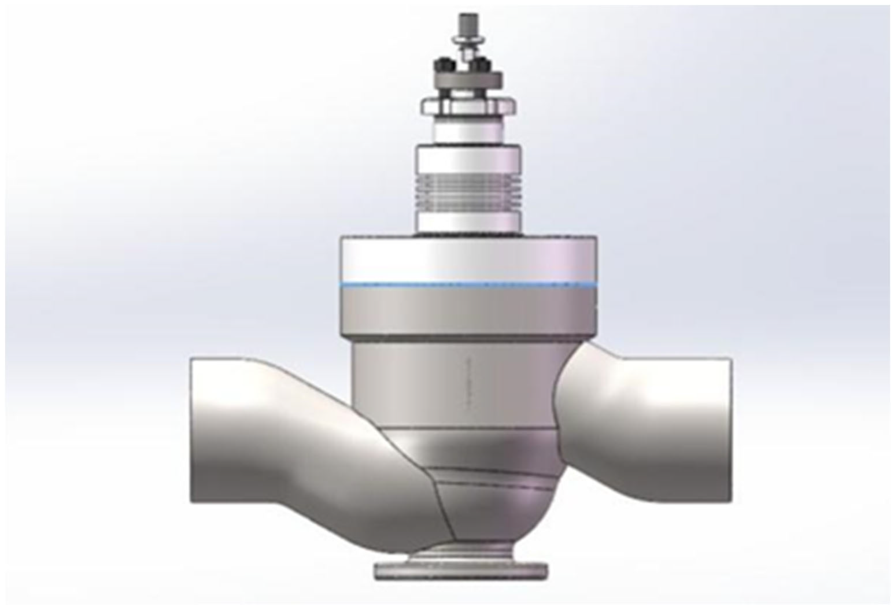
2. Structure and Operation of Control Valves

This study focuses on a DN150 Class1500 multi-stage sleeve control valve. This control valve is primarily used to depressurise high-pressure steam into low-pressure steam in steam pipelines. The valve has a 60 mm stroke, a high-temperature steam flow medium, and a linear flow characteristic for adjustment. Figure 1 shows the 3D model of the DN150, Class1500 multi-stage sleeve adjustment valve after eliminating and simplifying valve elements that are not relevant to the flow characteristics. High-temperature steam travels in the direction from the positive x-axis to the negative x-axis. The valve primarily controls the valve flow by altering the upper and lower valve core positions. The valve core moves up and down in the valve body, changing the flow area between the core and the valve seat, thereby limiting the flow. The first sleeve, second sleeve, third sleeve, valve seat, and stopper are shown in order from positive to negative on the x-axis for illustration. Figure 2 shows part of the SolidWorks-extracted 3D flow channel model. Using the flow channel of a control valve in the 100% open position as an example, the inlet and outlet effects of the flow channel will impact the flow in the control valve. The inlet and outlet are increased to six times the diameter in this study, and the sharp corners of the model, which are not ideal for dividing the mesh, are repaired reasonably.

The inlet pressure of the control valve is 9.8 MPa; the output pressure is 3 MPa; and the inlet temperature is 540 °C. The pressure difference between the front and back of the valve is substantial under these conditions, and steam will travel at a high velocity through the turbulent valve. The degree of steam turbulence is enhanced because of the internal throttling components of the control valve; hence, a turbulence model should be employed in the subsequent simulation.

3. Numerical Simulations

3.1. Basic Control Equations

The laws of mass action, momentum conservation, and energy conservation all apply to the movement of high-temperature steam. The high-temperature steam flow control equation is given below; steam is represented as a compressible ideal gas in this study, and there is no heat exchange with the valve wall.

$$\frac{\partial \rho }{\partial t}+\nabla \cdot (\rho \overrightarrow{V})=0$$

(1)

$$\frac{D\overrightarrow{V}}{Dt}={\overrightarrow{f}}_b-\frac{1}{\rho }\nabla p+\frac{\mu }{\rho }{\nabla }^2\overrightarrow{V}+\frac{1}{3}\frac{\mu }{\rho }\nabla (\nabla \cdot \overrightarrow{V})$$

(2)

$$\rho \frac{D}{Dt}(\stackrel{⌢}{u}+\frac{V^2}{2})=\rho {\overrightarrow{f}}_b\cdot \overrightarrow{V}+\nabla \cdot (\overrightarrow{V}\cdot {\tau }_{ij})+\nabla (\lambda \nabla T)+\rho \dot{q}$$

(3)

Equation (1) is the mass equation, also known as the continuum equation, in which ρ is the gas mass, and $\overrightarrow{V}$ is the velocity vector. Equation (2) is the momentum equation, in which ${\overrightarrow{f}}_b$ is the volume force, and μ is the dynamic viscosity coefficient. Equation (3) is the energy equation, in which $\stackrel{⌢}{u}$ is the internal energy per unit mass of fluid; ${\tau }_{ij}$ is the shear force; and T is the temperature (K) [27].

External heat exchange is not considered in this study; therefore, Equations (1) and (3) can be reduced to the following:

$$\nabla \cdot (\rho \overrightarrow{V})=0$$

(4)

$$\rho \frac{D}{Dt}(\stackrel{⌢}{\mu }+\frac{V^2}{2})=\rho {\overrightarrow{f}}_b\cdot \overrightarrow{V}+\nabla \cdot (\overrightarrow{V}\cdot {\tau }_{ij})$$

(5)

3.2. Turbulence Model

The standard k–ε turbulence model was chosen for this study to calculate the flow characteristics of the high-parameter control valve, because the medium of the control valve is steam, and the operating parameters are high. The standard k–ε turbulence model is commonly employed owing to its high accuracy and efficiency. Equations (6) and (7) show the standard k–ε transport model equations for the turbulent kinetic energy, k, and turbulent dissipation [28].

$$\frac{\partial }{\partial t}(\rho k)+\frac{\partial }{\partial x_i}(\rho k{u}_i)=\frac{\partial }{\partial x_j}[(\mu +\frac{{\mu }_t}{{\sigma }_k})\frac{\partial k}{\partial x_j}]+G_k+G_b-\rho \epsilon -Y_M$$

(6)

$$\frac{\partial }{\partial t}(\rho \epsilon )+\frac{\partial }{\partial x_i}(\rho \epsilon u_i)=\frac{\partial }{\partial x_j}[(\mu +\frac{{\mu }_t}{{\sigma }_{\epsilon }})\frac{\partial \epsilon }{\partial x_j}]+C_{1\epsilon }\frac{\epsilon }{k}(G_k+C_{3\epsilon }{G}_b)-C_{2\epsilon }\rho \frac{{\epsilon }^2}{k}$$

(7)

Here, $G_k$ describes the generation of turbulent kinetic energy, which can be calculated using the following equation:

$$G_k={\mu }_t\left(\frac{\partial u_i}{\partial x_j}+\frac{\partial u_j}{\partial x_i}\right)\frac{\partial u_i}{\partial x_j}$$

(8)

$Y_M$ is the expansion–diffusion term describing the effect of compressibility on the turbulence through expansion and diffusion; ${\sigma }_k$ and ${\sigma }_{\epsilon }$ are the turbulent Planck numbers of k and $\epsilon$, respectively (generally ${\sigma }_k$ = 1 and ${\sigma }_{\epsilon }$ = 1.3); and μ_t is the turbulent viscosity.

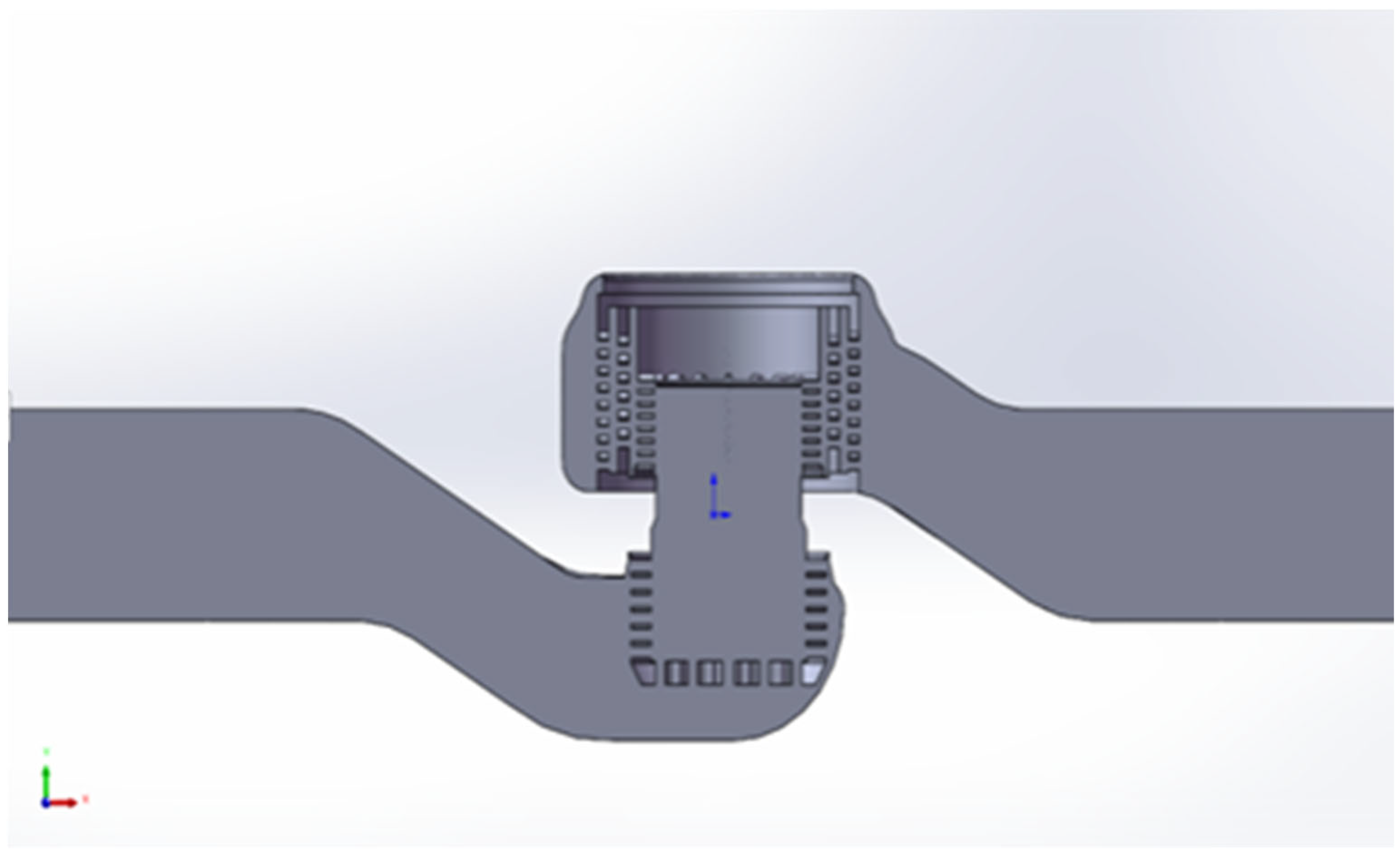
3.3. Meshing of the Flow Channels

The sleeve assembly and valve seat assembly have a high number of throttle apertures, and the structure is complex; therefore, the model is partitioned, as shown in Figure 2. The throttle orifices in the triple sleeve, valve seat, and plug are separated into different sections for regional mesh encryption using the ICEM CFD discrete mesh. After sub-regional processing, the mesh quality and accuracy are greatly improved, and the solution speed is considered.

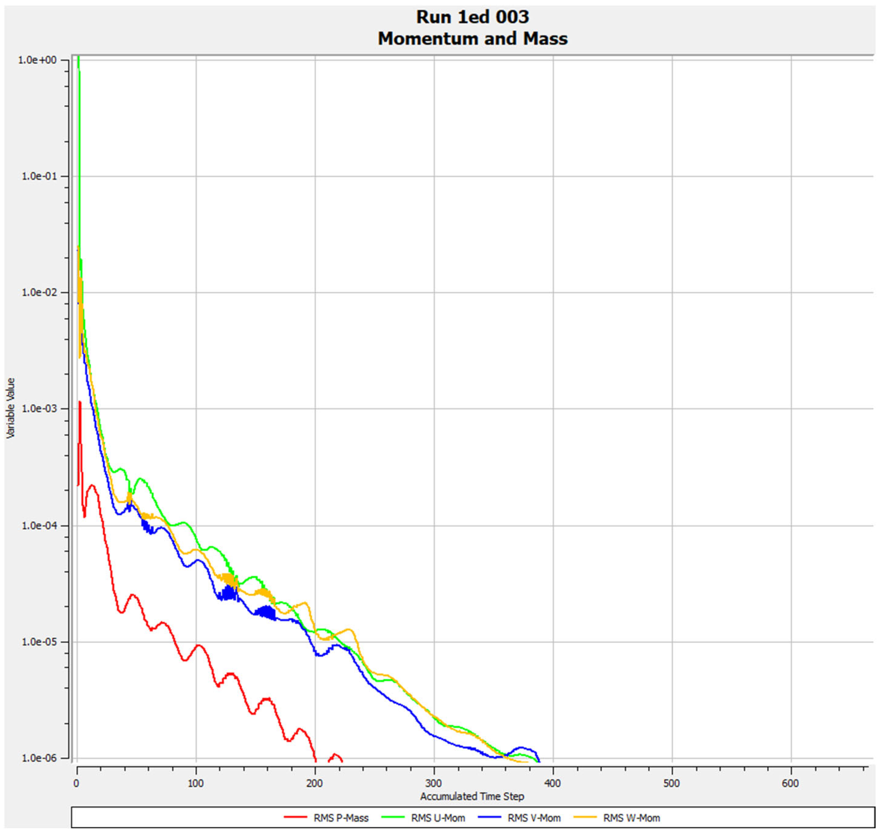
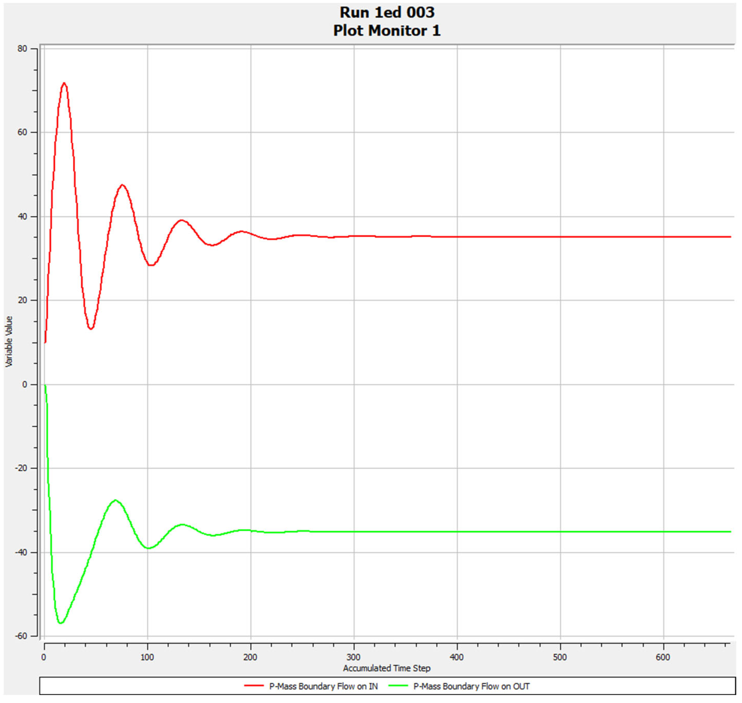
3.4. Setting the Boundary Conditions and Solver

The boundary conditions are determined based on the real operating conditions of the high-parameter control valve. The calculation program used in this study is CFX; the flow medium is Steam5 from the CFX material library; and the heat transfer model is the complete thermal model. The entire thermal model is based on the enthalpy model and considers the changes in the kinetic energy of the fluid. It can be used to calculate heat transfer in a high-speed and compressible flow. The inlet boundary condition is defined as a pressure boundary condition, and the total pressure is 9.8 MPa. The heat transfer is described based on a total temperature of 540 °C. The outlet boundary condition is set as a static pressure of 3 MPa. Finally, the solver is set to the upwind mode. The maximum number of iteration steps is set to 10,000, and the residual value is 10⁻⁶. The convergence is shown in Figure 3. Flow meters are installed at the inlet and outlet. Convergence is considered to be reached when the input and output flows are the same. The flow monitoring is shown in Figure 4.

4. Validation of the Numerical Model

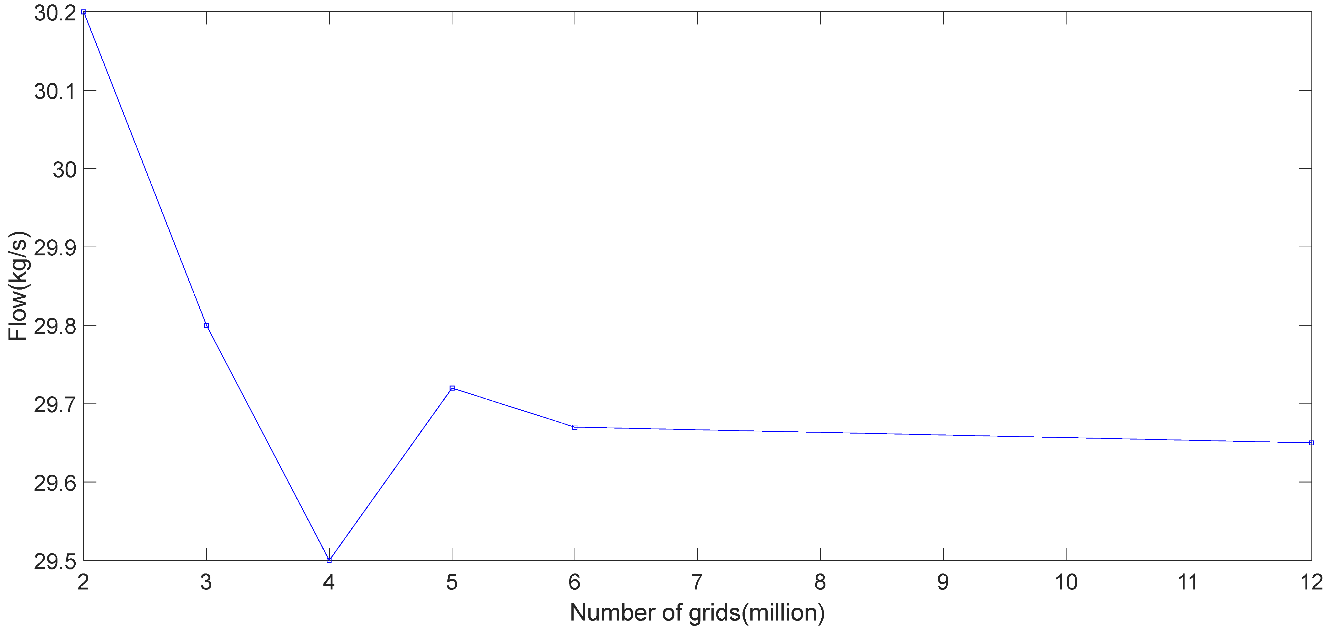
4.1. Grid-Independence Verification

As an example, a control valve with an opening of 80% is considered in this section. The boundary conditions are the same as above, and the flow rate is calculated for various grid numbers, as shown in Figure 5.

When the number of grids increases from 2 million to 12 million, the change in valve flow decreases gradually, but the overall difference in the numerical simulation results is less than 2%. Moreover, when the number of grids exceeds 3 million, the numerical simulation difference is less than 0.6%, indicating that when the number of grids exceeds 3 million, there is little influence on the calculation results. Therefore, a grid number of 3 million grids satisfies the grid independence criterion and is used for the computations.

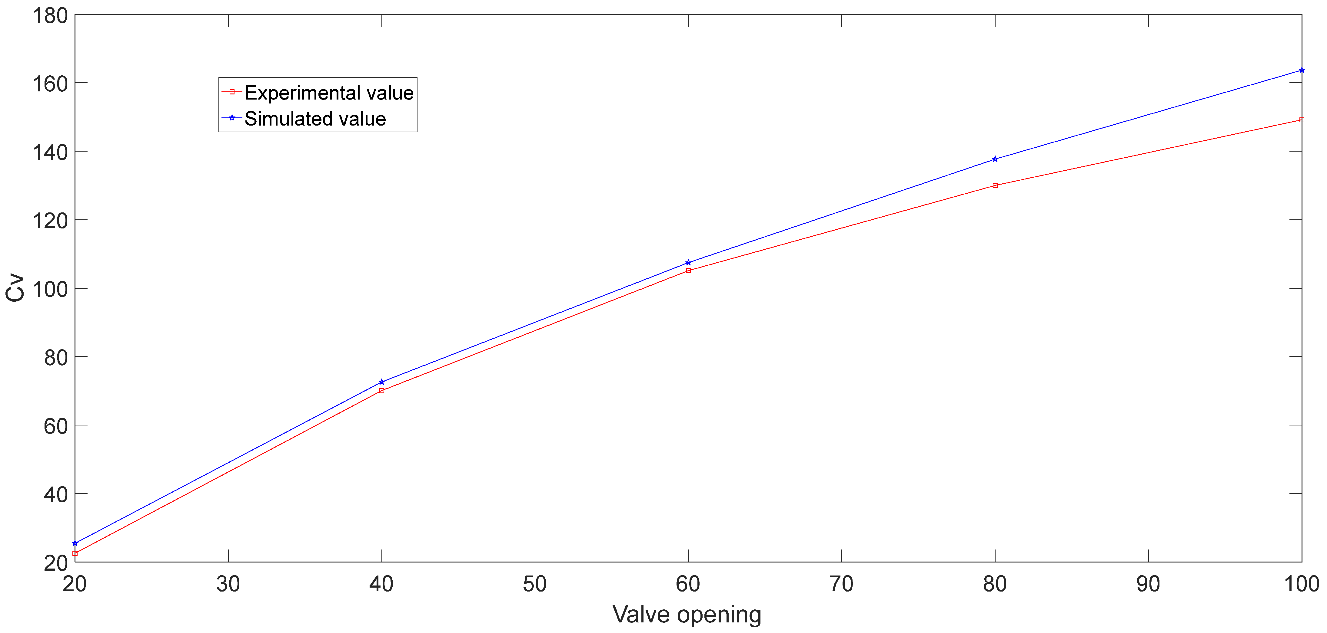
4.2. Calculation of the Flow Capacity of the Control Valve Numerical Model

The flow rate calculated by CFX is 30.8 kg/s at an intake pressure of 9.8 MPa, output pressure of 3 MPa, and steam temperature of 540 °C. The calculation approach uses the industrial process control valve GB/T 17213.2-2017 to evaluate the circulation capacity of the numerical model. [29] The compressible gas formula in the standard is used because the 540 °C steam is compressible. The basic flow model for a compressible fluid under turbulent conditions is calculated using Equation (9):

$$Q_S=C{N}_9{F}_P{p}_{1}Y\sqrt{\frac{X_{sizing}}{M{T}_1{Z}_1}}$$

(9)

where Q_S is the standard volume flow; C is the flow coefficient; N₉ is a numerical constant; F_p is the pipe geometry coefficient; p₁ is the inlet pressure; Y is the expansion coefficient; M is the molecular weight of the fluid; T₁ is the absolute inlet temperature; and Z₁ is the inlet compression factor.

Equation (9) can be transformed into the C_v calculation formula in Equation (10):

$$C_v=\frac{W}{N_6{F}_{P}Y\sqrt{X_{sizing}{P}_1{\rho }_1}}$$

(10)

where C_v is the valve flow coefficient, and N₆ is a numerical constant; N₆ = 2.73 can be found in standard Table I. Because the valve passage diameter and pipe diameter size are the same, F_p = 1 and X_TP = X_T. In this study, the control valve is a single-seat spherical valve with equal-bore sleeve internals. The standard in Table D.2 is consulted to obtain X_TP = X_T = 0.68.

The pressure drop ratio, X_sizing, is calculated according to Equation (11):

$$X_{sizing}=\{\begin{array}{l}x x<x_{choked}\\ x_{choked}x\ge x_{choked}\end{array}$$

(11)

$$x=\frac{p_1-p_2}{p_1}$$

(12)

The expansion coefficient, Y, is calculated according to Equation (13):

$$Y=1-\frac{x_{sizing}}{3x_{choked}}$$

(13)

The parameters presented in

Table 1. Parameter table.

Symbols	Description	Numerical Value
$p_1$	Inlet pressure	9.8 MPa
$p_2$	Outlet pressure	3 MPa
$N_6$	Numerical constants	2.73
$\gamma$	Specific heat ratio	1.315
$F_{\gamma }$	Specific heat ratio coefficient	0.939
$x_T$	Differential pressure ratio coefficient	0.68
$x_{sizing}$	Differential Pressure Ratio	0.639
$x_{choked}$	Blocking Differential Pressure Ratio	0.639
$x$	The ratio of actual differential pressure to absolute pressure	0.694
Y	Expansion Coefficient	0.677
$\rho$	Density	28.1
$F_p$	Pipe geometry coefficient	1
$W$	Mass flow rate	35.17

can be calculated using the operating conditions, physical characteristics, and above equations.

The full opening C_v is 163.7 according to the simulation results equation above. Using the above method and the simulated flow rates of different openings, the C_v of each opening can be calculated for the subsequent experimental control.

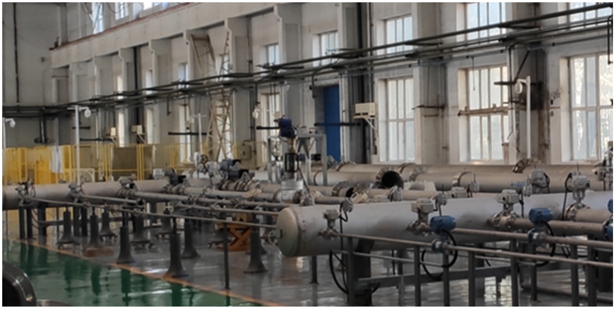
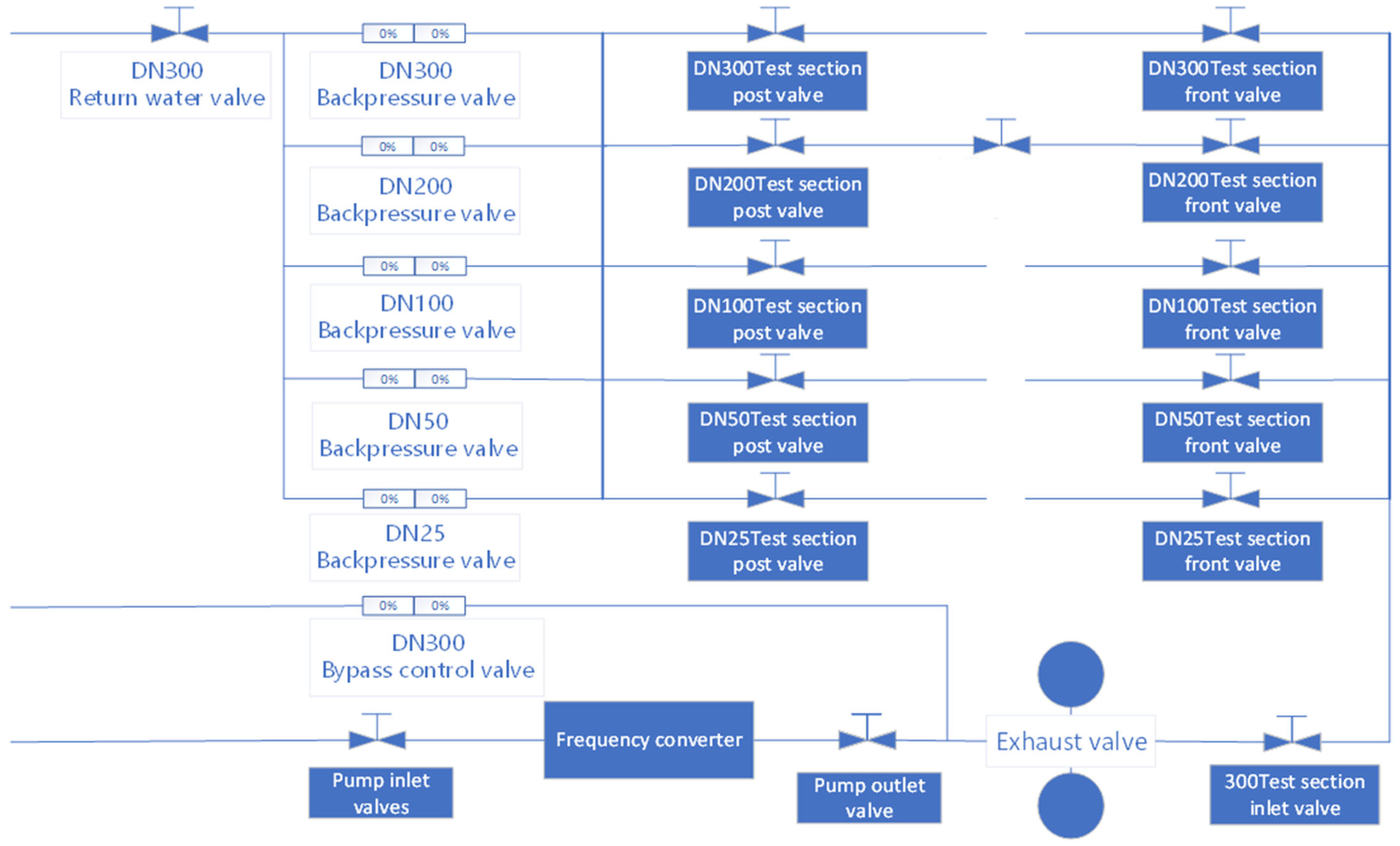
4.3. Control Valve Flow Resistance Experiments

Figure 6 shows the multi-stage sleeve control valve on the flow resistance test bench. The test bench is composed of the following parts (Figure 7): a water pump, the pump import and export valves, an inverter, a pressure stabilisation tank, a test section inlet valve, a flow meter, valves before and after the flow meter, test pipelines of various diameters, valves before and after the test section, a back pressure valve, and an exhaust valve. This test bench contains five different types of pipes; the control valve being tested is DN150 in size and is connected to the DN200 test part of the test bench via another piping system.

In the experiments, the steps are as follows:

• Test the pipelines. The goal control valve is connected to the circuit; the pump is turned on; the pump inlet and outlet valves are opened; the inverter frequency is set and started; and the flow-metered front and rear valves and the test section front and rear valves are opened successively. The return valve is opened after opening the DN200 back-pressure valve at a specific angle. The presence of leaks in the pipeline is checked; if none exist, the test is complete.
• Set the differential pressure before and after the valve to the desired value. The backpressure valve is adjusted three times for each opening degree to manage the pressure difference before and after the test segment. The differential pressure of the test section is set at 80, 100, and 120 kPa, and C_v was measured three times to obtain the average result.
• End the experiment. The frequency converter frequency is adjusted to 0 Hz; the bypass control valve is opened a certain angle; and the back pressure control valve of the pipeline being tested is opened fully. The pump is stopped after power-off processing to stabilise the pipe, and the pipeline is tested under test pressure relief after closing all of the valves. Finally, the system and operating table are exited, and the system is powered off.

Figure 8 shows a comparison between the experimental and simulation results. Because the roughness of the valve assembly is not considered in the simulation, the C_v error between the experiment and simulation ranges from 2% to 13% under various opening conditions. In addition, there is an error inside the electric actuator, which does not accurately open the valve to the specified opening. Consequently, the simulation method used in this study can be regarded as accurate.

5. Internal Flow Characteristics of a High-Parameter Multi-Stage Sleeve Control Valve

In the actual working conditions, the control valve generally operates at an opening of 30% to 70%; therefore, values of 20%, 40%, 60%, and 80% are considered in this study, with an opening of 100% being a critical opening in valve design. A single example is presented as illustrative. The effects of varying the opening on the flow characteristics of the valve are compared for openings of 20%, 40%, 60%, and 80%. This study primarily examines the pressure, velocity, and turbulent kinetic energy distribution in the valve under each opening to achieve a balance between the inlet and outlet flows and a residual value of 10⁻⁶ or less.

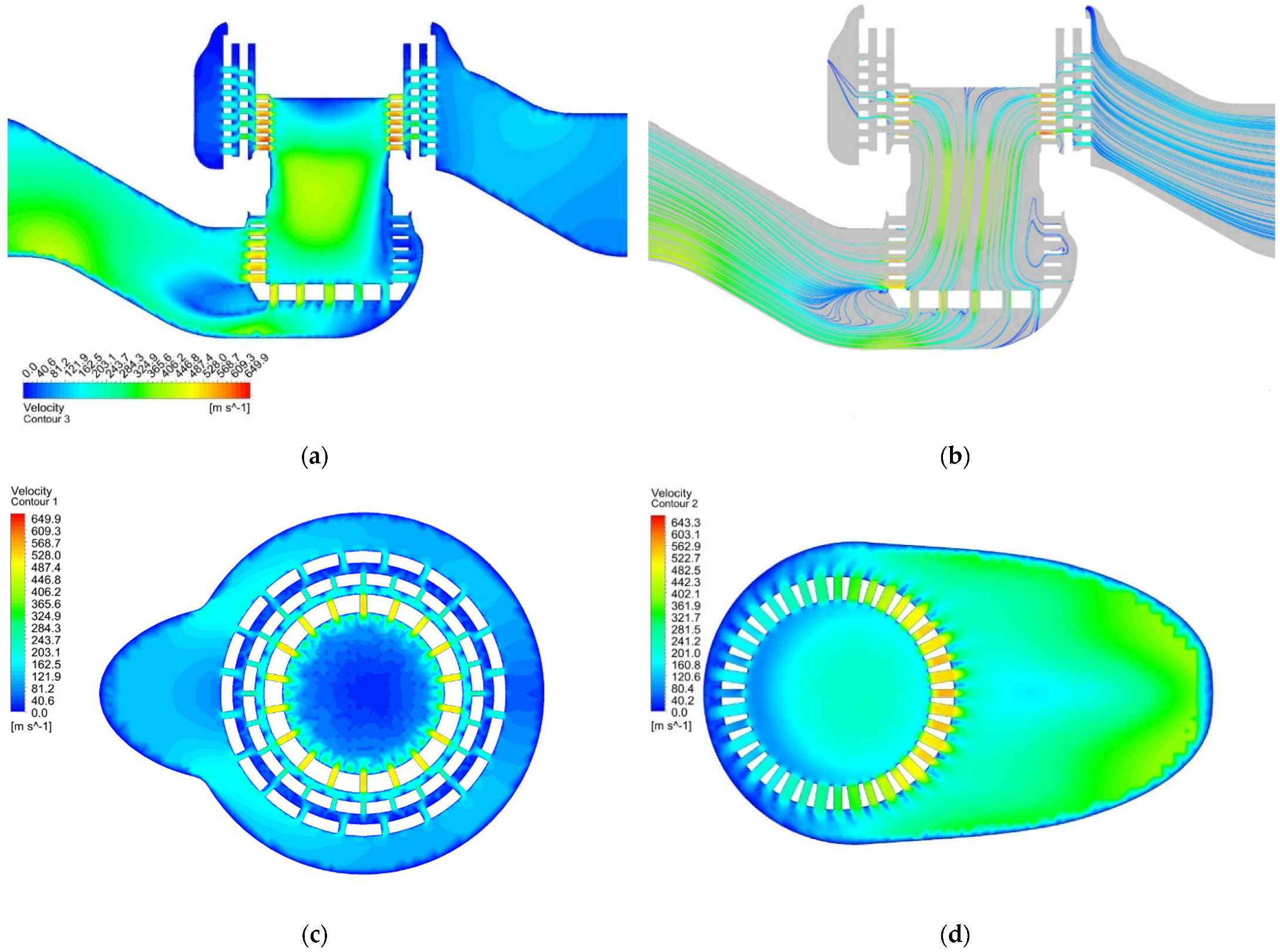
5.1. Flow Characteristics of Fully Open Valves

5.1.1. Analysis of the Complete Opening Speed of a Valve

The velocity diagram in the x-y plane in Figure 9a illustrates that when steam passes through the first sleeve, the flow cross-sectional area is reduced, causing the flow rate in the hole to increase to between 150 and 200 m/s. However, owing to the expansion of the steam circulation area created by the space between the sleeves, when the velocity of the gas is reduced, the flow rate of steam is reduced to below 100 m/s after the first sleeve layer. The steam then enters the second sleeve, and, owing to throttling, the velocity increases, resulting in a higher flow rate of approximately 300 m/s. At the throttle hole, the steam reaches a peak velocity of 650 m/s as it enters the third sleeve. Under the influence of the flow channel, steam flows along an arc. As shown in Figure 9a, steam converges in the middle of the sleeve in the area flush with the bottommost small hole and then flows along the flow channel direction, forming a relatively high-speed zone with a velocity of 350–450 m/s in the middle of the sleeve to the middle of the valve seat flow area. When steam passes through the throttle hole in the valve seat, the end near the outlet resembles steam travelling between the sleeves, with a peak velocity of approximately 600 m/s at the throttle hole, whereas a low-velocity zone appears at the end away from the outlet, with a velocity of 100 m/s. The flow is more turbulent because of the vortex development; hence, the speed is slower. The steam is disrupted by the high-parameter multi-stage sleeve control valve as well as the narrow orifice, as shown in Figure 9b, and vortices form inside the valve. Two larger vortices are formed in the bottom chamber of the valve body, as shown in Figure 9b. The steam is more turbulent when it flows into the small hole of the valve seat because it is disturbed by the inner wall surface of the ball spool inside the control valve sleeve, and two relatively powerful vortices are formed.

Figure 9c shows a sleeve cross-sectional x-z velocity cloud, and Figure 9d shows a valve seat x-z cross-sectional velocity cloud. The throttle hole of the three-layer sleeve has a progressive velocity in this order, and the gap between the two layers of the sleeve acts as a noticeable velocity buffer. The throttle holes are symmetrically distributed along the x-axis in the x-z cross-section of the valve seat, and the velocity is progressive from the positive to the negative direction of the x-axis; in other words, the throttle hole velocity distribution has a high symmetry effect.

5.1.2. Analysis of Turbulent Kinetic Energy under Full Opening of the Valve

Turbulence is defined as the development of fluid vortices of various sizes in a flow channel, leading to a random flow channel in which large-scale vortices convey energy to small-scale vortices that dissipate energy as heat. Because the intensity of the turbulence energy of steam in the flow channel of a high-parameter control valve causes pressure fluctuation and aerodynamic noise, it is important to study valves whose medium is steam. It is also important to analyse the intensity of the turbulence energy of steam in the flow channel of high-parameter control valves. The turbulent kinetic energy is a measure of the turbulence intensity of the fluid: the higher the turbulence energy, the higher the turbulence intensity, and vice versa.

The turbulent kinetic energy cloud diagram in the x-y plane is used as an example to explore the turbulent kinetic energy distribution of steam in the regulating valve body in greater detail. The maximum turbulent kinetic energy of this valve at an opening of 100% is 1.27 × 10⁴, as illustrated in Figure 10. Compared to Figure 9b, the area where steam occurs on the symmetry surface inside the valve body correlates to the area where the turbulence energy is higher, suggesting that the turbulence during steam vortex generation is severe, resulting in more violent pressure pulsations. Consequently, minimising the intensity of the steam vortex inside the valve body is critical for lowering the valve noise. Furthermore, in the outlet direction, the maximum value of the turbulent kinetic energy is found in the throttle hole of the valve seat. However, the scale is smaller, and a larger-scale vortex is generated when the medium flows out of the valve seat in contact with the spherical valve wall, indicating that the flow of steam changes after encountering the obstruction of the valve body wall, increasing the turbulent kinetic energy of the steam. Another large-scale vortex emerges from the medium flowing out of the sleeve throttle hole, hedging at a greater speed, and then flowing back to the spool after passing through the throttle hole of the valve seat and undergoing a spherical valve wall collision.

The components in the valve body disturb the steam to generate a high-speed flow and vortex, which intensifies the steam turbulence. Strong turbulence causes the pressure of steam to pulsate, which causes noise. As a result, valve noise reduction efforts can be focused on the back wall of the valve cavity and bottom of the valve body.

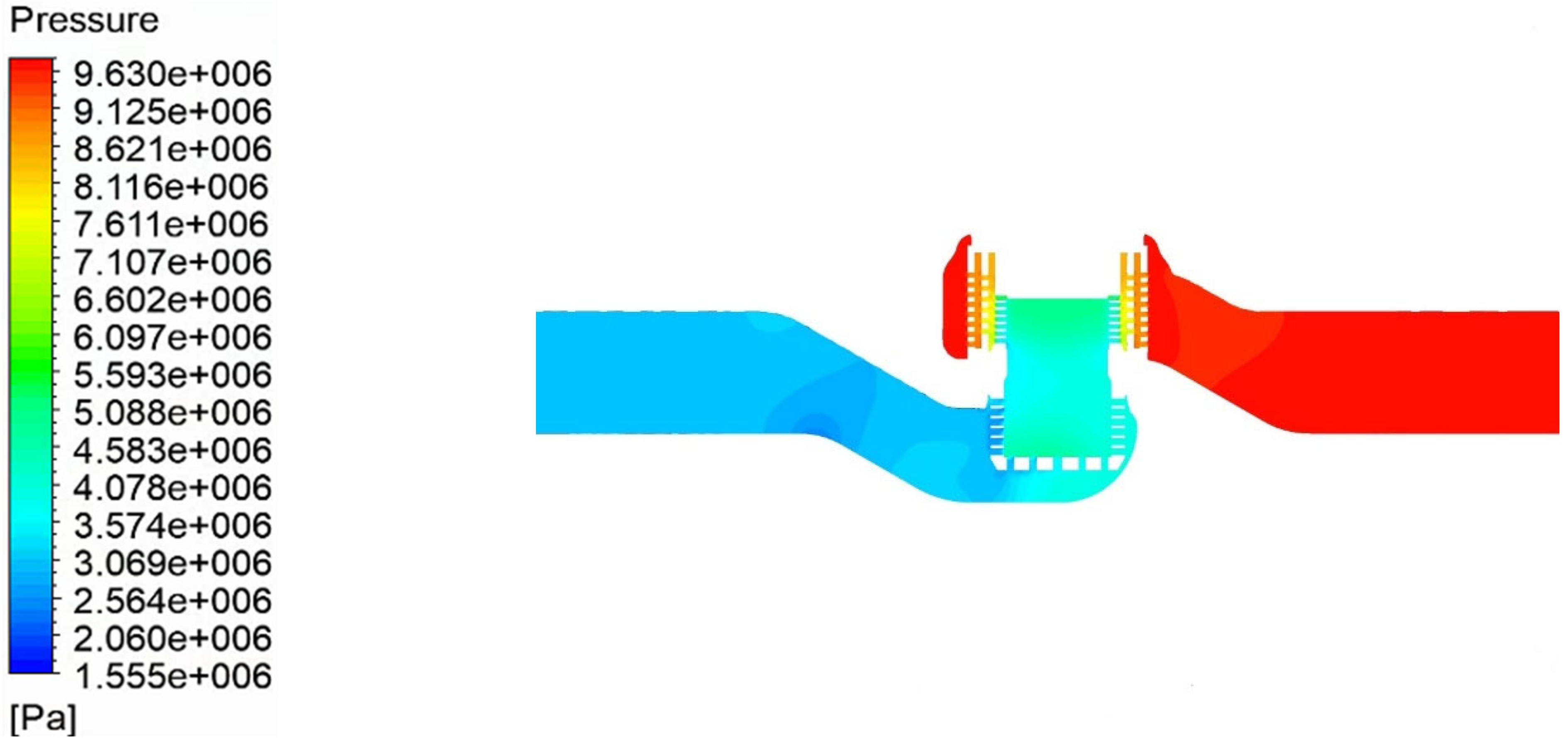
5.1.3. Analysis of the Full Opening Pressure of a Valve

Figure 11 shows the static pressure distribution clouds of steam in the x-y plane of the flow route to examine the static pressure distribution of steam in the flow path of a high-parameter multi-stage sleeve control valve. As shown in Figure 11, all three layers of the sleeve exhibit pressure drop effects; however, the pressure drop in the first layer is not noticeable, and the pressure loss in the third layer is the largest. Following the turn, the flow rate and pressure both recover, which is consistent with the velocity diagram.

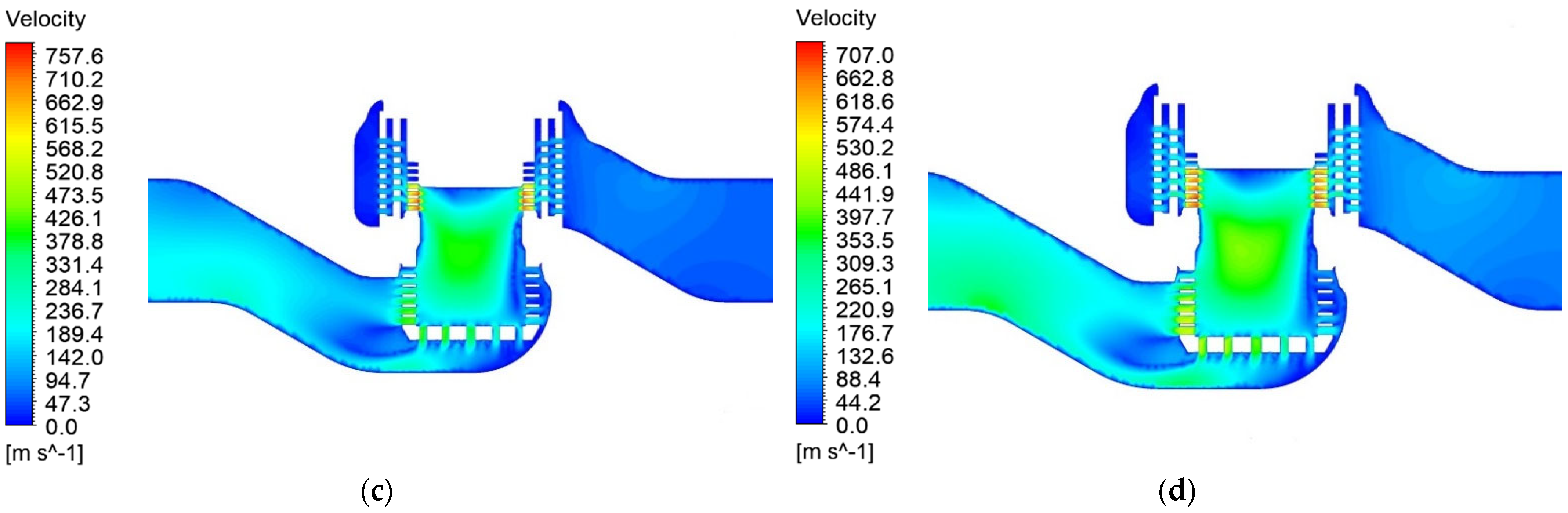
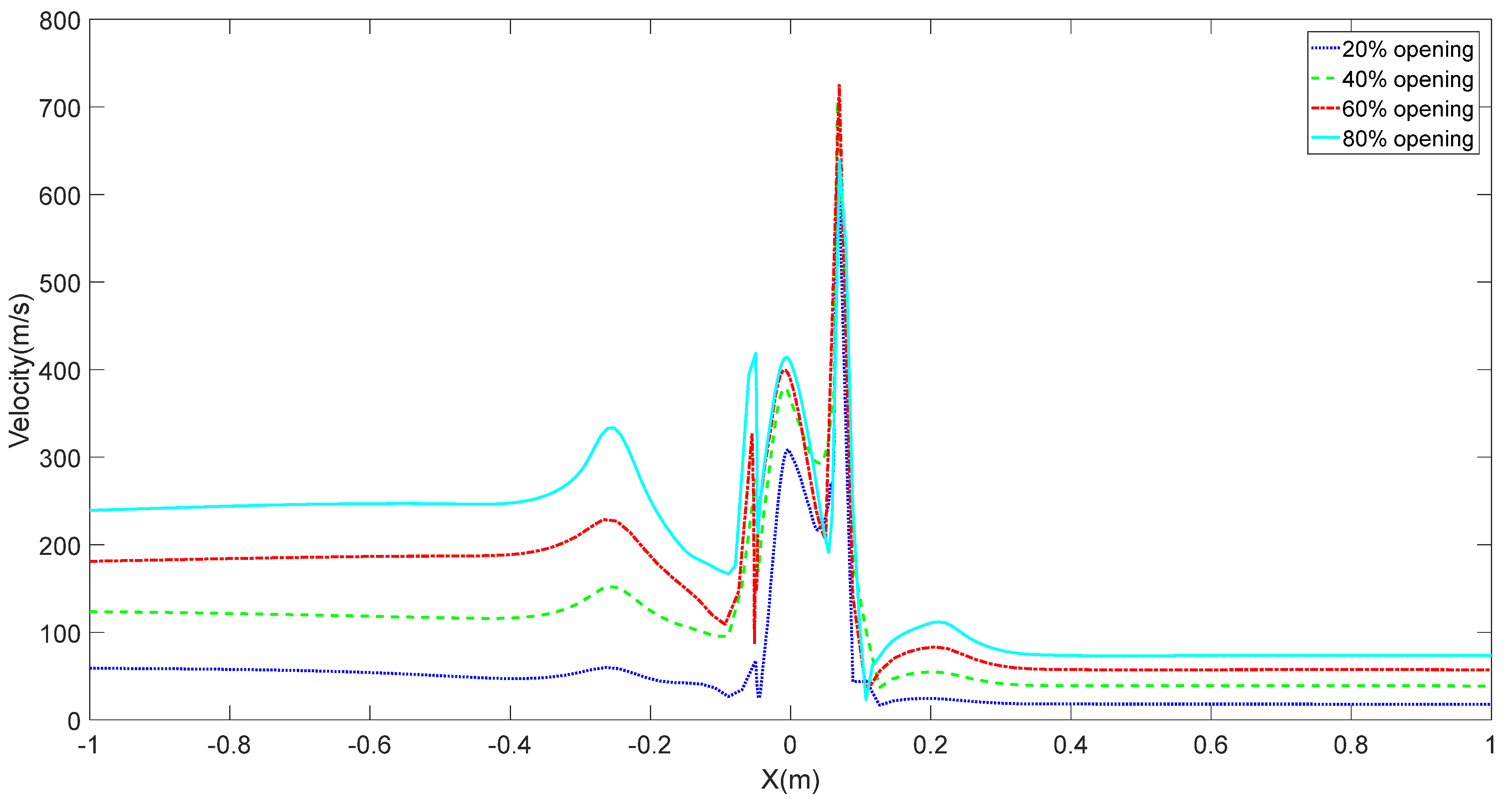
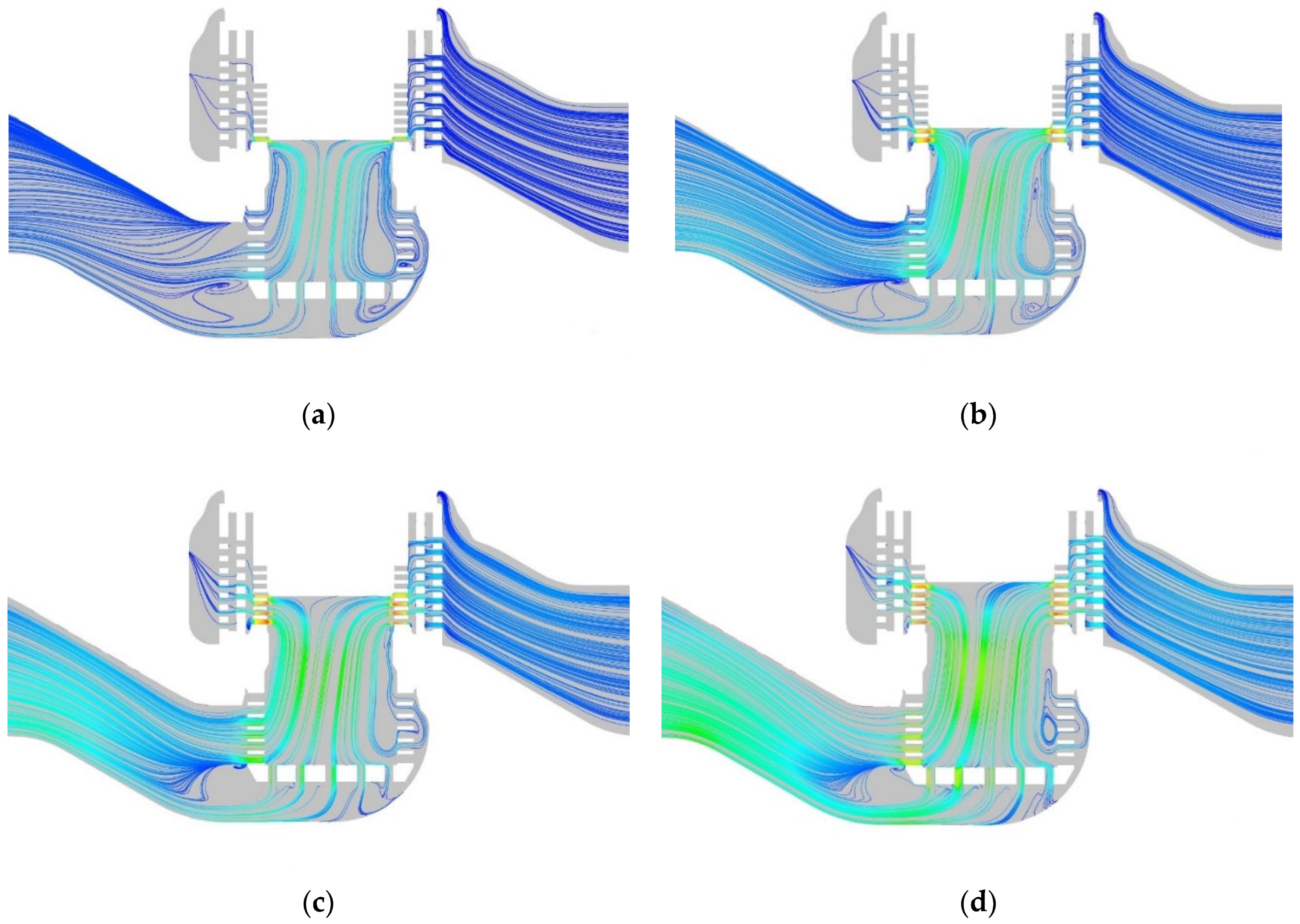
5.2. Analysis of the Velocity Field with Varying Degrees of Opening

For flow field computations, control valve openings of 20%, 40%, 60%, and 80% are chosen based on the actual working conditions of the control valve. Figure 12 shows the throttling velocity of the three layers of the sleeve from the outside to the inside in increasing order, with the third layer of the sleeve having the largest throttling effect when the valve opening approaches 20%. The velocity in the central zone steadily increases as the opening degree increases, whereas the high flow velocity region gradually expands. Because of the complex flow within the multi-stage pressure-drop control valve, the monitoring curve is set from the inlet to the outlet, as shown in Figure 13, with four peak points: x = 0.1 is the maximum peak point corresponding to the inlet side of the sleeve throttle hole; the x = 0 peak point corresponds to the internal area of the sleeve; the x = −0.1 corresponds to the throttle hole of the valve seat in the direction of the outlet; and the point at x = −0.25 corresponds to the outlet bend. The flow rate at the sleeve throttle hole does not comply with this law because the opening degree is different, and the number of throttle holes connected to the sleeve part is different, resulting in different circulation areas. Therefore, this does not comply with the expected trend of faster flow rates with higher opening degrees.

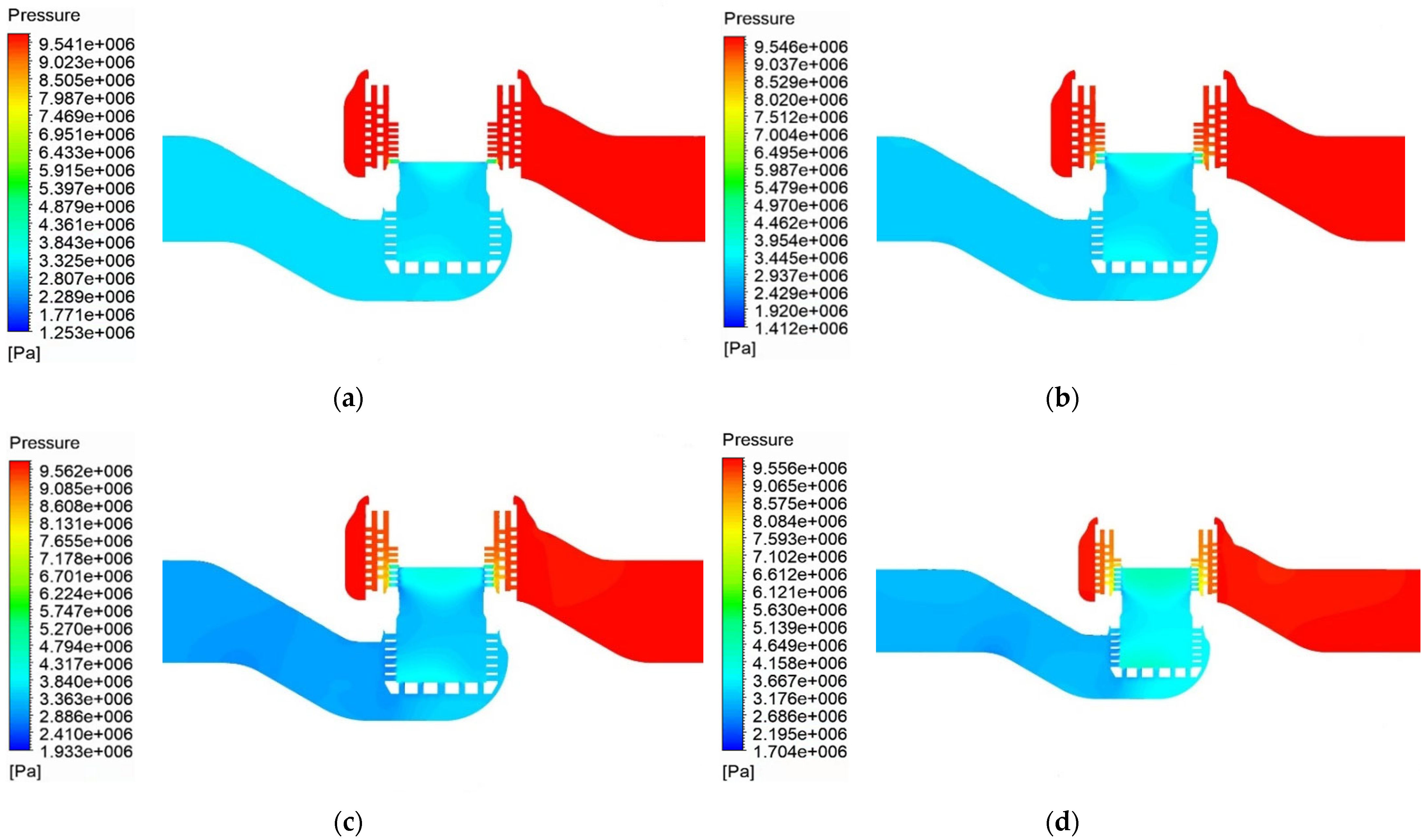
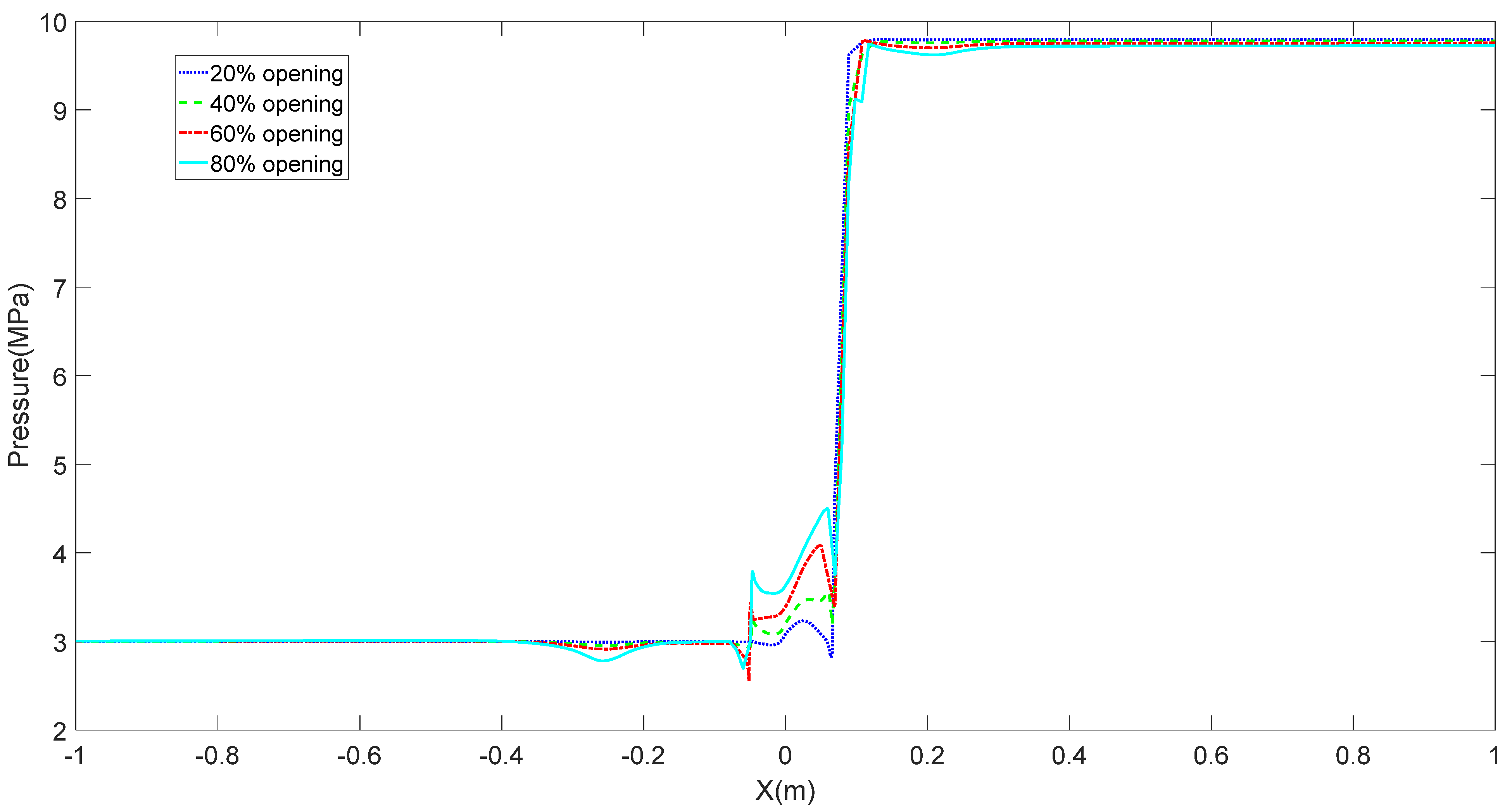
5.3. Analysis of the Pressure Field with Different Opening Degrees

Regulating valves openings of 20%, 40%, 60%, or 80% are selected for the pressure field simulations based on the real working conditions of the regulating valve. The valve x-y plane pressure distribution is shown in Figure 14 to illustrate the pressure changes after the steam enters the regulating valve. From the inlet to outlet monitoring curve shown in Figure 15, the pressure cloud from the inlet to the outlet exhibits a downward trend. The opening of the first two layers of the sleeve reduces the role of the pressure drop with the opening of the first two layers of the sleeve to reduce the role of the pressure. The monitoring curve clearly shows that, at an opening of 80% at x = 0.15 m, the second layer sleeve still has a definite pressure decrease, while the middle two openings have modest changes in slope but no clear steps. Through the throttling effect, a pressure of 9 MPa can be decreased to roughly 3.5 MPa. This is also seen in the velocity detection curve, which is quite acute at the larger pressure drop and corresponds to the pressure detection curve. The local high pressure generated at the top and bottom of the valve cavity can be observed in the pressure cloud diagram, and the range of the high-pressure area gradually broadens as the opening degree increases. The two peaks of the pressure monitoring curve, x = 0.05 and x = −0.05, indicate that as the opening degree increases, the pressure values at the top and bottom of the valve chamber also increase. In general, the impact on the pressure drop of the high-parameter multi-stage sleeve adjustment valve is visible, and the pressure fluctuation is not significant.

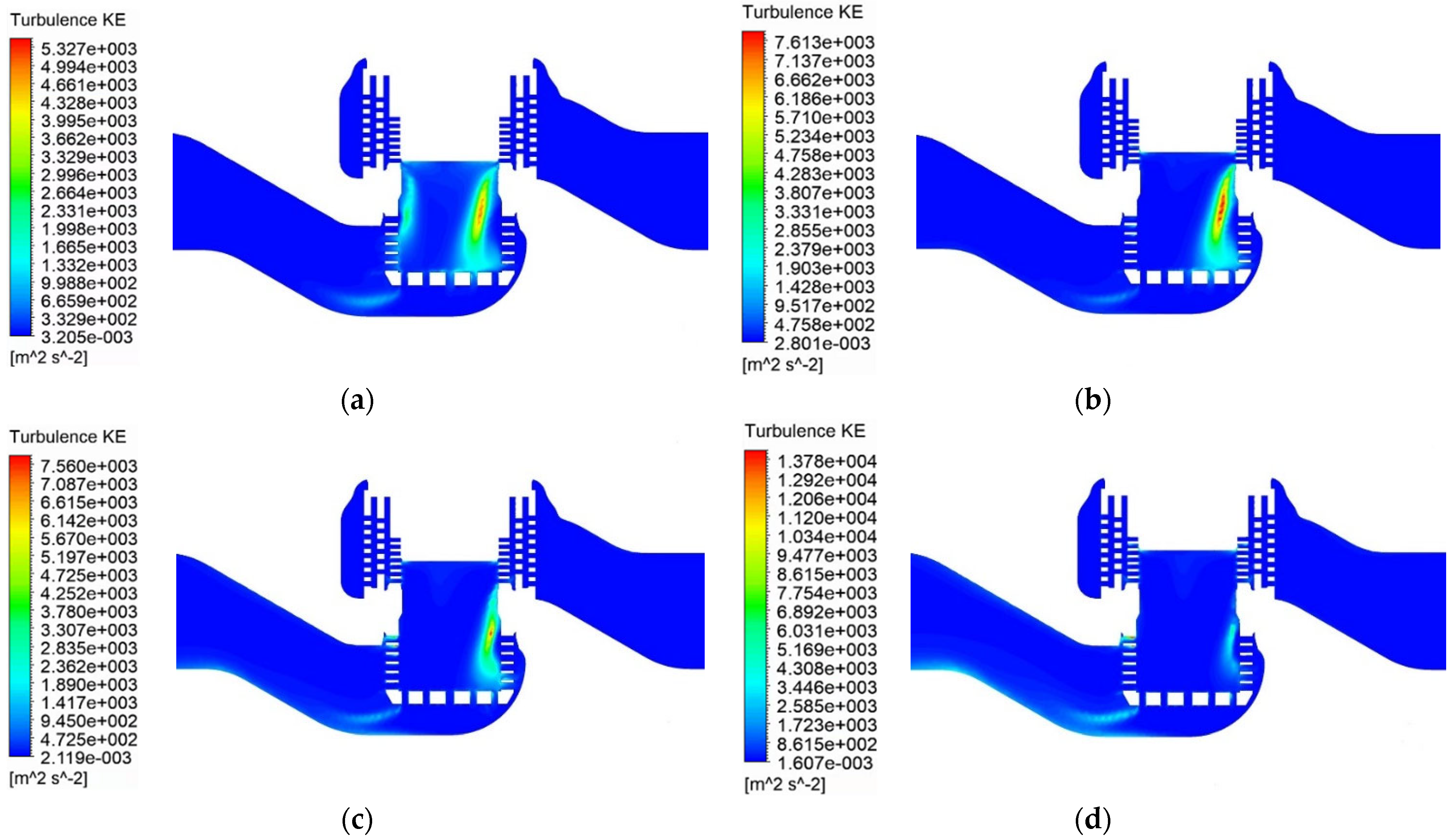
5.4. Analysis of the Turbulent Kinetic Energy for Various Opening Degrees

The pressure field simulation computation is carried out by selecting openings of the regulating valve of 20%, 40%, 60%, and 80% depending on the actual working conditions of the regulating valve. The distribution of the turbulent kinetic energy in the x-y plane of the valve is shown in Figure 16. According to the previous discussion of turbulent kinetic energy, the generation of turbulent kinetic energy is often directly related to the vortex. Therefore, to show the media flow line in the valve in the x-y plane, the turbulent kinetic energy cloud is shown in Figure 17. The results show that the lower the opening percentage, the larger the region of turbulent kinetic energy; however, the extreme value is reduced. The equivalent surface in the upper part of the throttle hole of the valve seat in the outlet direction determines the extreme value points, and the maximum turbulent kinetic energy area is more clearly visible under an opening of 80%, where the extreme value is larger, but the influence range is very small. The rear wall surface of the valve chamber and the bottom of the valve body in the outlet direction have a larger influence range. Figure 17 shows that these two locations have significant vortex formation, and the complete opening is an excellent match for the turbulence energy analysis.

6. Conclusions

This study primarily used flow resistance experiments to determine the C_v of the target regulating valve, and the results were compared to the calculated and simulated C_v values to verify the accuracy of the numerical simulation. CFX software was used to analyse the flow characteristics of the fully open high-parameter multi-stage sleeve regulating valve as an example, compared with openings of 20%, 40%, 60%, and 80%. The effects of adjusting the valve opening degree on the flow characteristics can be summarised as follows:

• The velocity of each portion of the valve increases with the opening degree of the valve. The velocity at the sleeve throttle hole, on the other hand, is slightly different, with a higher opening in the middle and a lower opening on both sides.
• The pressure at each component of the valve increased as the opening degree increased, and the pressure drop effect in the first two layers of the sleeve intensifies.
• The extreme value of turbulence energy increases as the opening degree increases; the vortex range shrinks; and the extreme point of turbulence energy is located in the throttle hole at the top of the valve seat output direction.

A large range of vortex formation occurs primarily in the valve cavity back wall surface and the bottom of the valve body in the outlet direction. Vortexes are an important factor in the generation of turbulence and cause of aerodynamic noise; therefore, reducing the control valve aerodynamic noise can focus on the two large vortex areas, reduce the impact of the vortex range, and achieve comprehensive noise reduction. A throttling orifice can be added at the outlet, which can effectively reduce the noise in the direction of the outlet. The thickness of the valve body can also be increased, which can effectively reduce noise penetration.

The outlet vortex flushes the bottom of the spherical valve body, and after a wide range of vortices, erosion of the valve seat throttle hole in the valve chamber will occur. The top and bottom of the valve cavity have a local high pressure generated after sleeve throttling owing to the vortex effect, which forms a distinct low-pressure area, and the corresponding spool, stem, and plug will be subjected to increased force; the subsequent design should consider these essential elements. The steam streaming from the sleeve is turbulent, which will readily disrupt the components inside the valve, generating vibration, which is another major source of noise.

References

1. Ogawa, K. Effect of semicircular fins on noise reduction in butterfly valve cavitation under a biased velocity distribution condition. Proc. Int. Instrum. Symp. 2010, 482, 1–30. [Google Scholar]
2. Youn, C.; Asano, S. Flow Characteristics of Pressure Reducing Valve with Radial Slit Structure for Low Noise. J. Vis. 2008, 11, 357–364. [Google Scholar] [CrossRef]
3. Qian, J.Y.; Zhang, M. Mach number analysis on multi-stage perforated plates in high pressure reducing valve. Energy Convers. Manag. 2016, 119, 81–90. [Google Scholar] [CrossRef]
4. Tu, S.; Wang, C. Study on flow-induced vibration of cage type control valve. Am. Inst. Phys. 2013, 1547, 131–135. [Google Scholar]
5. Wang, Y.; Hu, J.H. Design and research of noise elimination and vibration reduction sleeve in control valve. Fluid Mach. 2013, 41, 19–22. [Google Scholar]
6. Xu, X.G.; Wang, T.L. High temperature and high pressure drop multistage sleeve regulator noise suppression research. Autom. Instrum. 2016, 1, 4–6. [Google Scholar]
7. Jin, Z.J.; Wei, L.; Chen, L.L.; Qian, J.Y.; Zhang, M. Numerical simulation and structure improvement of double throttling in a high parameter pressure reducing valve. J. Zhejiang Univ. Sci. A 2013, 14, 137–146. [Google Scholar] [CrossRef] [Green Version]
8. Hou, C.W.; Qian, J.Y.; Chen, F.Q.; Jiang, W.K.; Jin, Z.J. Parametric analysis on throttling components of multi-stage high pressure reducing valve. Appl. Therm. Eng. 2018, 128, 1238–1248. [Google Scholar] [CrossRef]
9. Jin, Z.J.; Chen, F.Q. Numerical analysis of flow and temperature characteristics in a high multi-stage pressure reducing valve for hydrogen refueling station. Int. J. Hydrogen Energy 2016, 41, 5559–5570. [Google Scholar] [CrossRef]
10. Yu, J.M.; Gao, G.; Zhang, H. Analysis of the influence of sleeve structure on throttling characteristics of valves. Reneng. Dongli. Gongcheng. 2019, 34, 14–20. [Google Scholar]
11. Rammohan, S.; Saseendran, S.; Kumaraswamy, S. Effect of multi jets on cavitation performance of globe valves. J. Fluid Sci. Technol. 2009, 4, 128–137. [Google Scholar] [CrossRef] [Green Version]
12. Tang, Y.; Zheng, J.H. Analysis on flow characteristics of multi-stage control valve based on CFD. J. Chengdu Aeronaut. Vocat. Tech. Coll. 2016, 32, 56–58. [Google Scholar]
13. Sreekala, S.K.; Thirumalini, S. Effect of cage configurations on flow characteristics of globe valves. World J. Eng. 2016, 13, 61–65. [Google Scholar]
14. Kim, H.S. Analysis of Flow Characteristics and Effects of Turbulence Models for the Butterfly Valve. Appl. Sci. 2021, 11, 6319. [Google Scholar]
15. Qiu, C.; Jiang, C.H.; Zhang, H. Pressure Drop and Cavitation Analysis on Sleeve Control Valve. Processes 2019, 7, 829. [Google Scholar] [CrossRef] [Green Version]
16. Chern, M.J.; Hsu, P.H.; Cheng, Y.J. Numerical study on cavitation occurrence in globe valve. J. Energy Eng. 2013, 139, 25–34. [Google Scholar] [CrossRef]
17. Yaghoubi, H.; Madani, S.A.H.; Alizadeh, M. Numerical study on cavitation in a globe control valve with different numbers of anti-cavitation trims. J. Cent. South Univ. 2018, 25, 2677–2687. [Google Scholar] [CrossRef]
18. Huovinen, M.; Kolehmainen, J.; Koponen, P. Experimental and numerical study of a choke valve in a turbulent flow. Flow Meas. Instrum. 2015, 45, 151–161. [Google Scholar] [CrossRef]
19. Beune, A.; Kuerten, J.G.M.; Schmidt, J. Numerical calculation and experimental validation of safety valve flows at pressures up to 600 bar. AIChE J. 2011, 57, 3285–3298. [Google Scholar] [CrossRef]
20. Chattopadhyay, H.; Kundu, A.; Saha, B.K. Analysis of flow structure inside a spool type pressure control valve. Energy Convers. Manag. 2012, 53, 196–204. [Google Scholar] [CrossRef]
21. Zhe, L.; Ma, C.; Xu, H. Numerical and experimental studies on hydrodynamic characteristics of sleeve control valves. Flow Meas. Instrum. 2017, 53, 279–285. [Google Scholar]
22. Asim, T.; Mishra, R.; Oliveira, A. Effects of the geometrical features of flow paths on the flow capacity of a control valve trim. J. Pet. Sci. Eng. 2018, 172, 124–138. [Google Scholar] [CrossRef] [Green Version]
23. Chern, M.J.; Wang, C.H.; Lu, G.T. Design of cages in globe valve. Proc. Inst. Mech. Eng. Part C 2015, 229, 476–484. [Google Scholar] [CrossRef]
24. Pan, X.; Wang, G.; Lu, Z. Flow field simulation and a flow model of servo-valve spool valve orifice. Energy Convers. Manag. 2011, 52, 3249–3256. [Google Scholar] [CrossRef]
25. Rafaqat, R.; Khan, A.A. MHD compressible fluid with variable thermal conductivity through a ciliated channel. Adv. Mech. Eng. 2021, 13, 16878140211010003. [Google Scholar] [CrossRef]
26. Khan, A.A.; Rafaqat, R. Effects of radiation and MHD on compressible Jeffrey fluid with peristalsis. J. Therm. Anal. Calorim. 2021, 143, 2775–2787. [Google Scholar] [CrossRef]
27. Launder, B.E.; Spalding, D.B. Lectures in Mathematical Models of Turbulence; Academic Press: New York, NY, USA, 1972; pp. 152–162. [Google Scholar]
28. Hongwei, W. Fluid Mechanics as l Understand It, 2nd ed.; National Defense Industry Press: Beijing, China, 2019; pp. 88–99. [Google Scholar]
29. Jiong, W.; Minghua, L. GB/T 17213.2–2017. Industrial Process Control Valves Part 2–1: Flow Capacity Formula for Calculating Fluid Flow under Installation Conditions; Shanghai Industrial Automation Instrumentation Research Institute: Shanghai, China, 2017. [Google Scholar]
Figure 1. 3D model of the multi-stage sleeve control valve.
Processes 10 01504 g001
Figure 2. 3D flow channel model.
Processes 10 01504 g002
Figure 3. Residual monitoring.
Processes 10 01504 g003
Figure 4. Flow monitoring.
Processes 10 01504 g004
Figure 5. Grid independence verification.
Processes 10 01504 g005
Figure 6. Flow and resistance-to-flow test bench.
Processes 10 01504 g006
Figure 7. Schematic of the test bench.
Processes 10 01504 g007
Figure 8. Comparison of experimental and simulated values.
Processes 10 01504 g008
Figure 9. Valve speed simulations at full opening: (a) x-y plane velocity cloud; (b) x-y plane velocity streamlines; (c) sleeve cross-section x-z velocity cloud; (d) valve seat x-z cross-sectional velocity cloud.
Processes 10 01504 g009
Figure 10. Turbulent kinetic energy cloud of the fully open valve.
Processes 10 01504 g010
Figure 11. Static pressure distribution cloud map of a fully open valve.
Processes 10 01504 g011
Figure 12. Velocity clouds for different opening percentages: (a) 20%; (b) 40%; (c) 60%; (d) 80%.
Processes 10 01504 g012aProcesses 10 01504 g012b
Figure 13. Velocity monitoring.
Processes 10 01504 g013
Figure 14. Pressure clouds with different opening percentages: (a) 20% opening; (b) 40% opening; (c) 60% opening; (d) 80% opening.
Processes 10 01504 g014
Figure 15. Pressure monitoring curve.
Processes 10 01504 g015
Figure 16. Turbulent kinetic energy clouds with different opening degrees: (a) 20% opening; (b) 40% opening; (c) 60% opening; (d) 80% opening.
Processes 10 01504 g016
Figure 17. Streamline diagrams with different opening degrees: (a) 20% opening; (b) 40% opening; (c) 60% opening; (d) 80% opening.
Processes 10 01504 g017