
Exploring Systemic Risk Dynamics in the Chinese Stock Market: A Network Analysis with Risk Transmission Index

Abstract
:1. Introduction
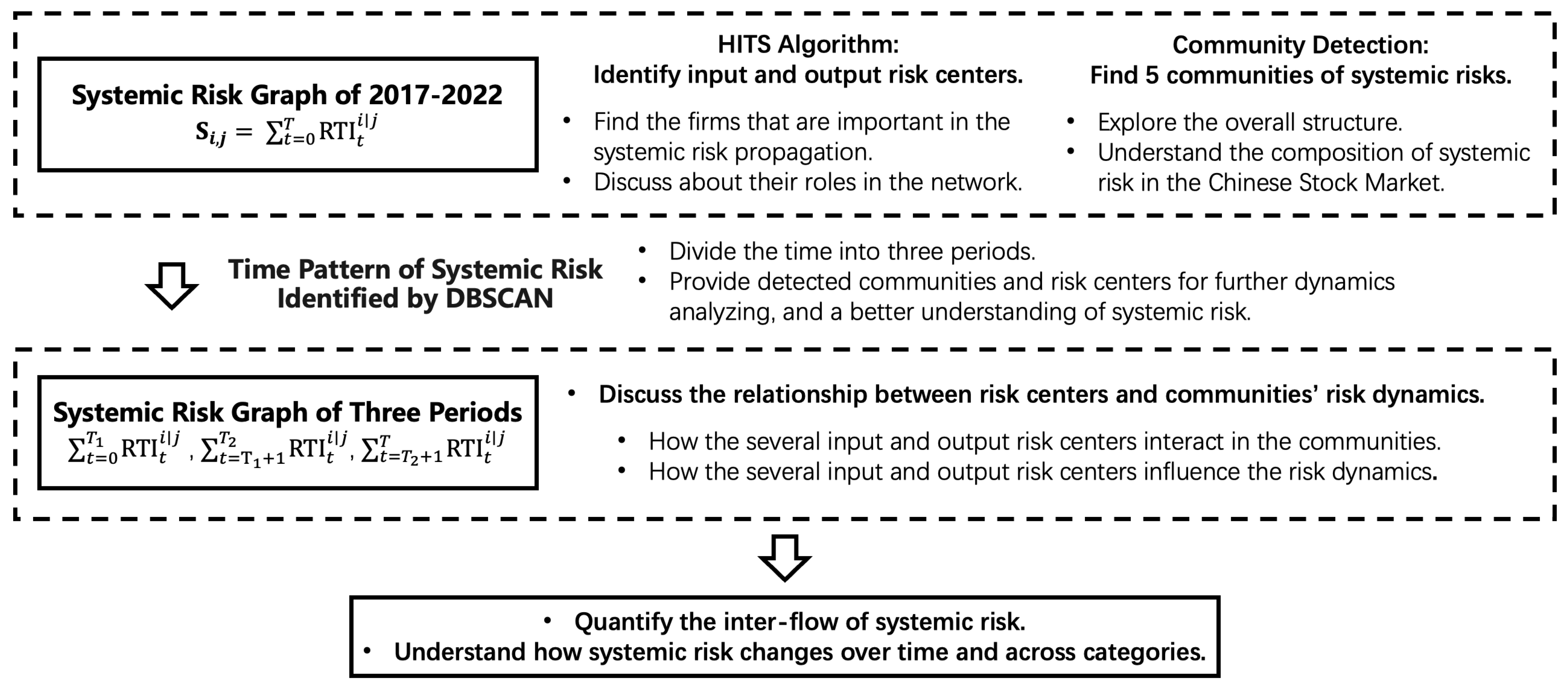
- How can we quantify the inter-flow of systemic risk in the network of Chinese stock markets? We construct a systemic risk network for individual stocks, observe how systemic risk propagates within the stock market, explore the major risk output and input centers, and analyze the primary constituents of systemic risk in the Chinese stock market.
- How does the major systemic risk contributors influence the systemic risk across communities and over time? We employ clustering algorithm on the risk dynamics over time to obtain small time periods, and then find out how the major risk centers behave regarding both detected communities and time periods in the system risk network we construct for the Chinese stock market.
2. Materials and Methods
2.1. CoVaR Based on a Single Index Model
2.1.1. Estimation of VaR and CoVaR
2.1.2. Risk Fluid in the Network
2.2. Systemic Risk Network Analysis
2.2.1. Identifying Input and Output Risk Centers by HITS Algorithm
| Algorithm 1 HITS |
|
2.2.2. Identify Constituents of Systemic Risk by Community Detection Algorithm
| Algorithm 2 Community detection. |
|
2.2.3. Identify Time Pattern of Systemic Risk by DBSCAN Algorithm
| Algorithm 3 DBSCAN |
|
3. Results
3.1. Sample and Data
3.1.1. Data Description
- The “Pareto Principle” or the “80/20 Rule” is evident in the Chinese stock market. This principle, first proposed by the renowned Italian economist Vilfredo Pareto in 1897, states that 20% of the population holds 80% of the wealth. In the context of the stock market, this translates to the fact that 20% of the stocks tend to be profitable in the long term, while the remaining 80% often incur losses (Wu et al. 2010). This suggests that using a smaller subset of stocks to represent the overall market is reasonable. By calculating the long-term returns for each stock based on the annual average closing prices in 2012 and 2022, we observe that approximately 73% of the stocks in the market have zero or negative returns, which aligns with the “80/20 Rule”.
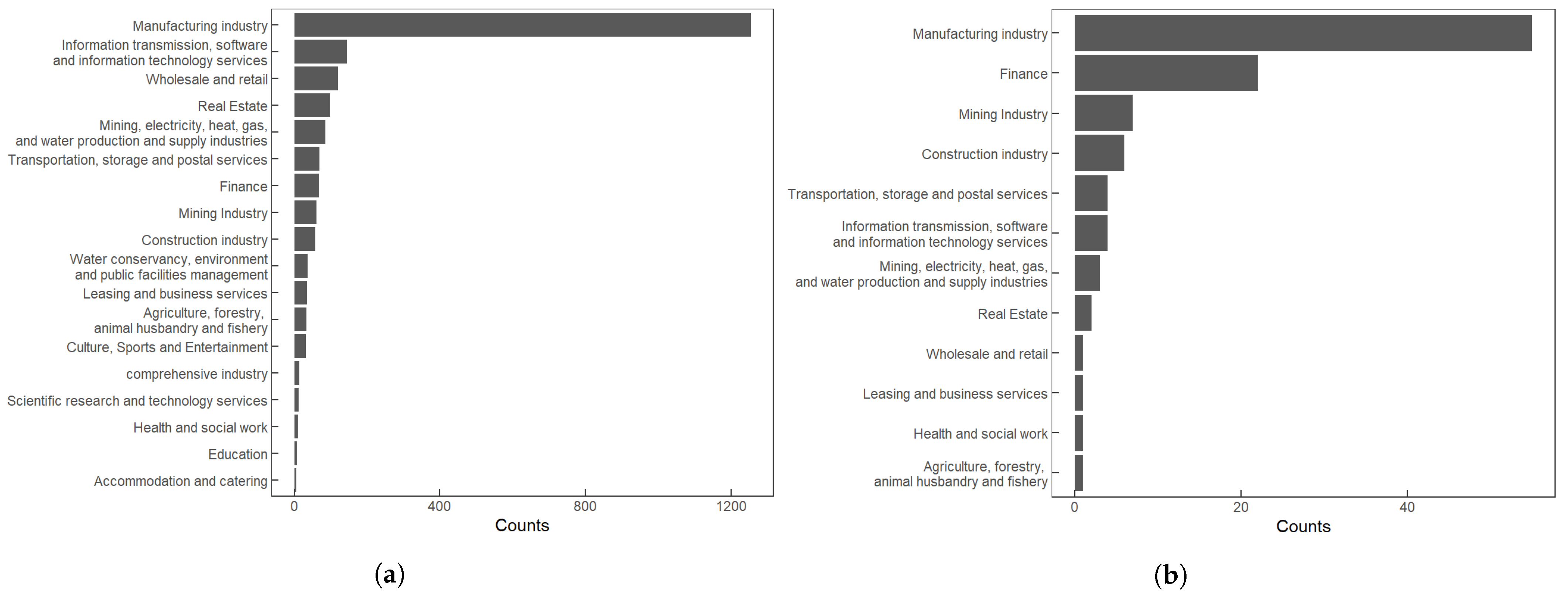
- The industry distribution of the selected stocks is similar to that of the broader market. As depicted in Figure 3a,b, the industry distribution of the 107 stocks chosen in this study closely mirrors the industry distribution of the overall market, effectively reflecting the operational characteristics of the securities market.
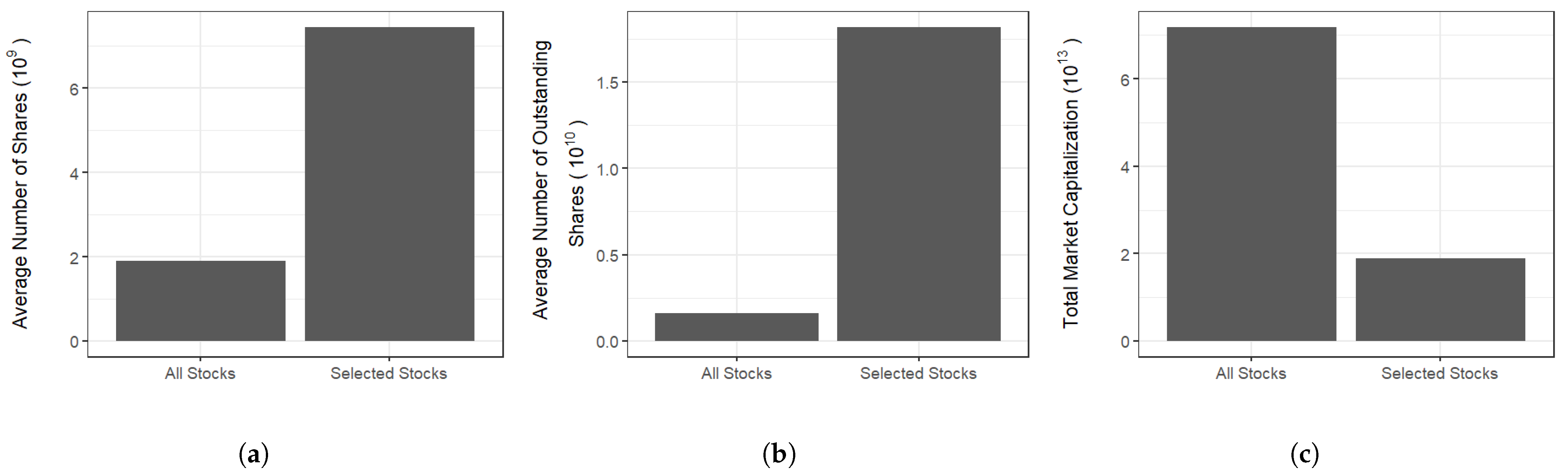
- The selected stocks in our study exhibit significant market capitalization and liquidity. As shown in Figure 2a,b, using the average number of shares per company as a measure of market size, the selected stocks in this study have an average number of shares that is 3.91 times higher than the market average. Additionally, using the latest available data on the number of outstanding shares as a measure of liquidity, the average number of outstanding shares for the selected stocks in this study is 11.42 times higher than the market average.We do not choose the Shanghai 50, CSI 300, or STAR 50 for the following reasons:
- Shanghai 50: The selection criteria for Shanghai 50 are essentially the same as those for Shanghai 180, but it comprises only 50 stocks, which provides a less comprehensive representation of the stock market due to its smaller sample size.
- CSI 300: Within the CSI 300, 30% of the stocks come from the financial industry, which does not align well with the industry distribution of the overall market.
- STAR 50: The STAR 50 index consists of the 50 largest STAR Market-listed companies, which are relatively newer and may not provide sufficient data for analysis due to their recent establishment.
3.1.2. Macroeconomic Indicators
- Foreign Trade Indicators reflect the foreign trade status of a country or region, the level of foreign trade activities, and international competitiveness.
- Real Estate-Related Indicators reflect the activities and investment conditions in the real estate market.
- Consumer-Related Indicators reflect the consumption behavior and capacity of residents, indicating the strength of economic consumption activities and changes in consumer confidence.
- Energy Logistics-Related Indicators reflect the activity level and demand situation in the financial market’s energy and logistics sectors.
- Commodity-Related Indicators reflect the supply and demand relationships, cost pressures, and market price fluctuations of commodities. They hold significant reference value for economic analysis and decision-making.
- Financial Market Indicators reflect the operational status of the financial market and interest rate levels.
- Macroeconomic Overall Indicators reflect the overall economic scale and growth conditions of a country or region, indicating the overall economic development and the relative contributions of various industries.
3.1.3. Data Preprocessing
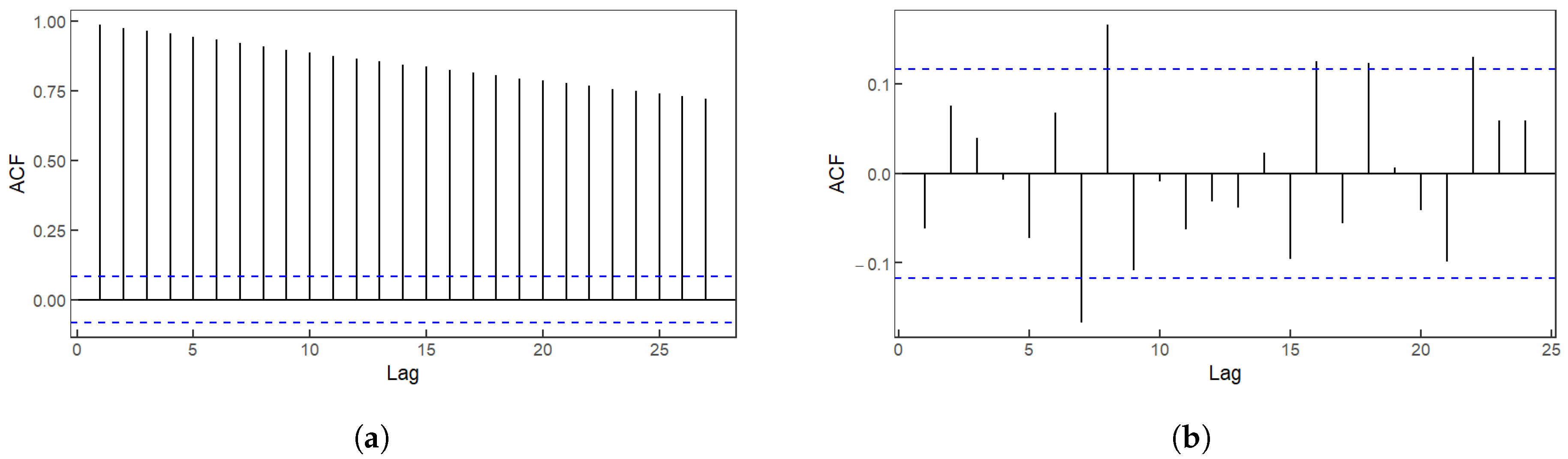
- Unprocessed Stock Price Data. Before any transformation, the ADF tests show that only five stocks’ price series out of all the stocks are stationary. Subsequently, we take the logarithm of the price data and then differentiate it. The ADF tests are performed again, and the results indicate that, after the stationarity transformation, all stocks reject the non-stationary null hypothesis, thus rendering the price series stationary. Consequently, we utilize the rolling forecast to obtain biweekly stock price data with the rolling window being 5 years. We illustrate the transformation progress with the ACF plot of Shanghai Pudong Development Bank (C600000, Shanghai, China) before and after stationarity transformation in Figure 4.
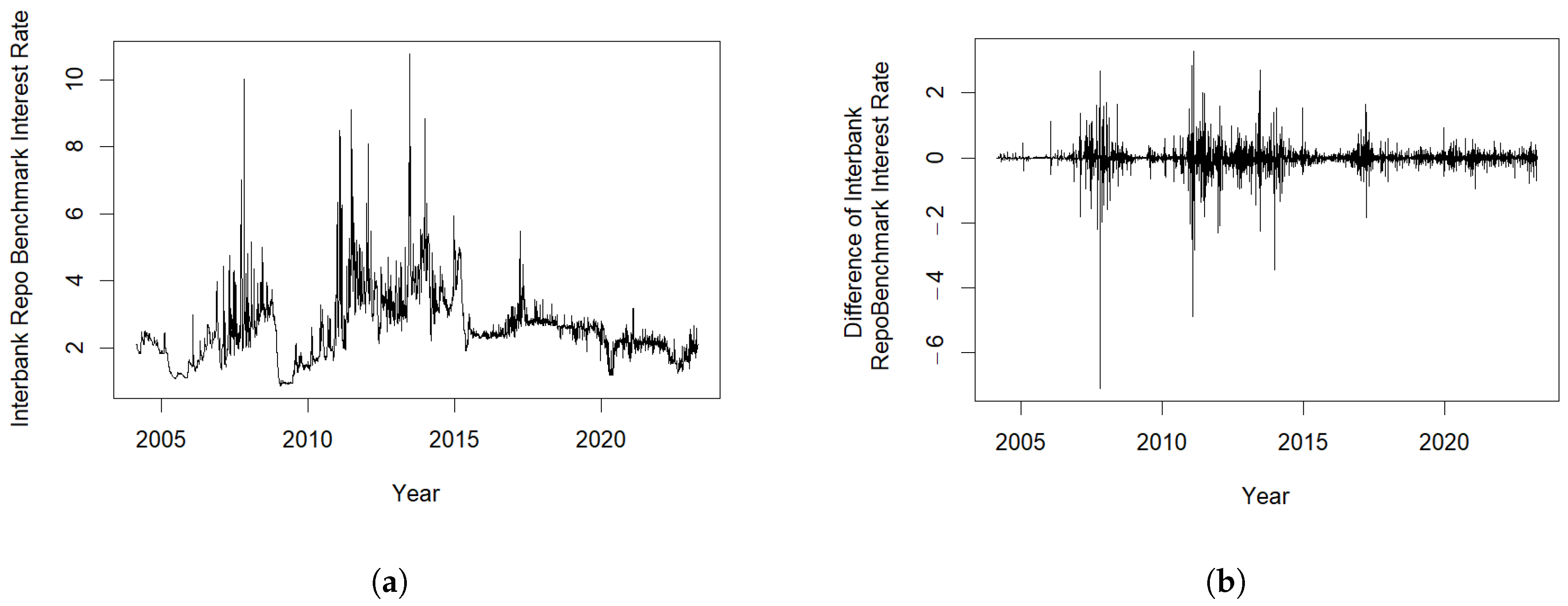
- Macroeconomic Indicators. Among all the daily and monthly data, only the monthly CPI data pass the ADF test. By observing ACF and PACF plots and relying on empirical knowledge, we determine the appropriate transformation methods for each indicator. After applying these transformations, all data become stationary.Regarding quarterly data, due to the large time intervals and relatively limited data spanning only 10 years with 45 data points, the ADF test alone cannot effectively confirm the stationarity of the data. Additionally, there is significant volatility in the quarterly data during the period from 2020 to 2022, which we believe can influence the overall stationarity of the data. Therefore, we employ empirical rules and refer to ACF and PACF plots as well as the reduction in p-values from the ADF tests to decide on the data transformation methods, which partially improve data stationarity. The specific methods used for stationarity transformation of the macroeconomic data are detailed in Table 1. Moreover, we illustrate such effect of 1st difference for Interbank Repo Benchmark Interest Rate in Figure 5.Finally, we utilize cubic spline interpolation to adjust all indicators to a biweekly time cycle.
- Three-factor Model and Balance Sheet. The ADF tests show that all the data are stationary at a significance level of 0.05, and no further stationarity processing is required.
3.2. Systemic Risk Network Analysis of the Chinese Stock Market
3.2.1. Feasibility Testing of QR–Lasso Model
3.2.2. Feasibility Testing of Systemic Risk Network
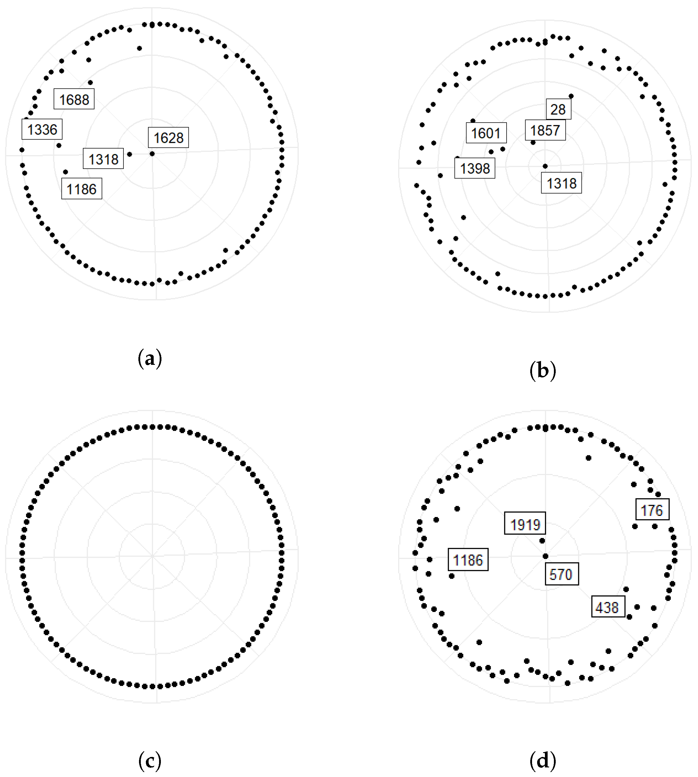
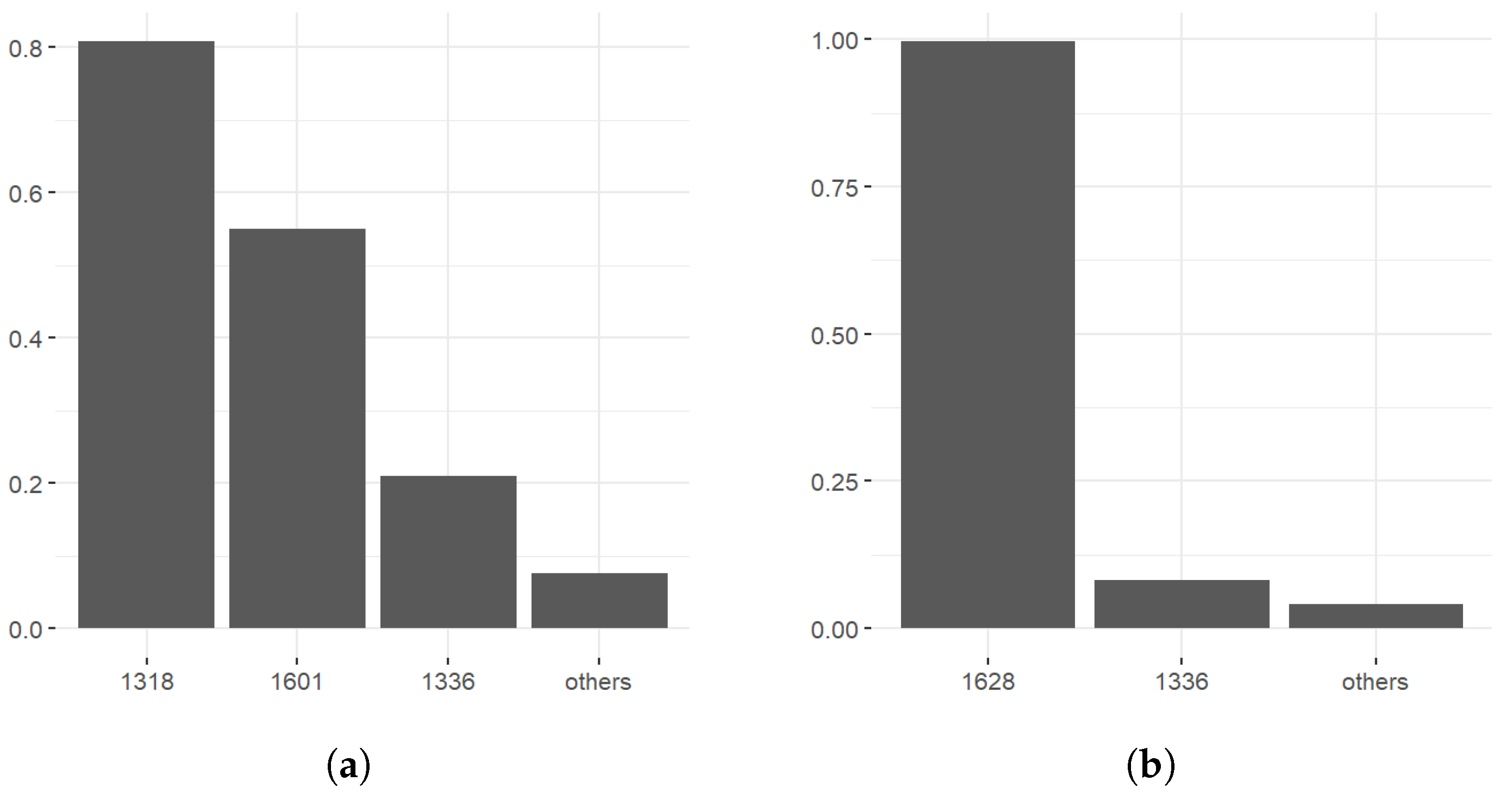
3.2.3. Primary Output and Input Centers of Systemic Risk
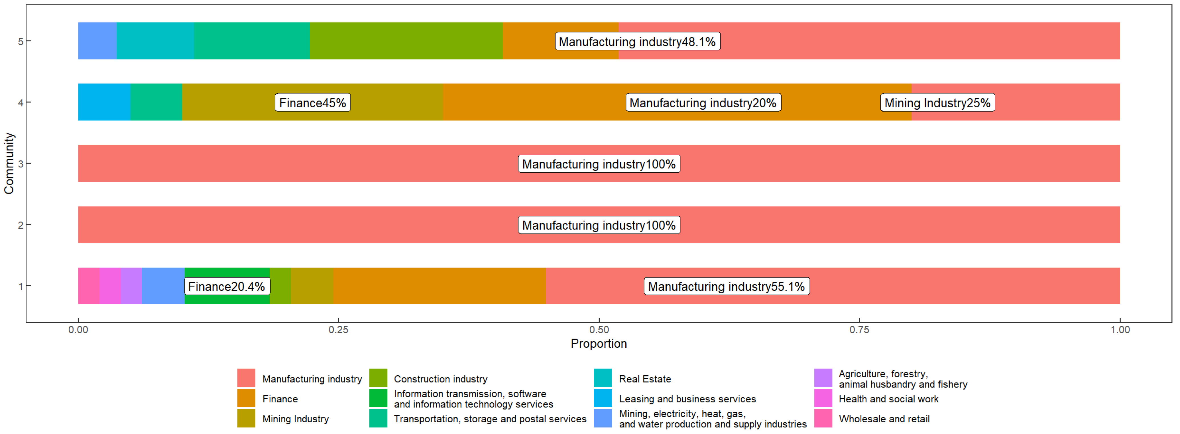
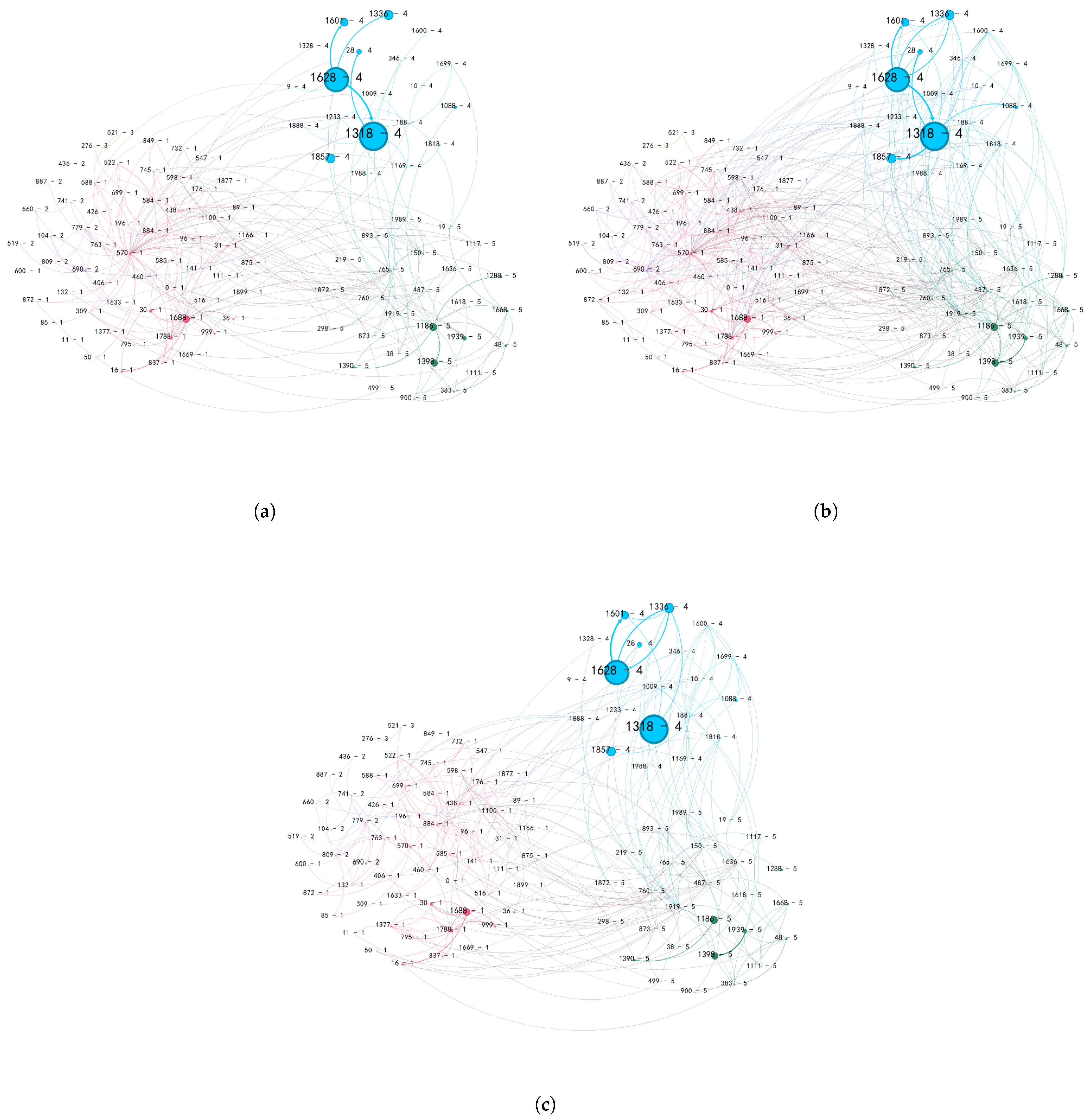
3.2.4. Industry Composition of Systemic Risk
- Communities 1, 2, and 3 exhibit a diverse composition, encompassing emerging industries such as fin-tech, biopharmaceuticals, optical fiber, and emerging manufacturing sectors. Community 2 comprises automotive manufacturing entities, exemplified by corporations such as SAIC Motor Group (104, Shanghai, China) and Fuyao Glass Industry Group Company Ltd (660, Fuzhou, China). Conversely, Community 3 is primarily characterized by healthcare enterprises, notably encompassing pharmaceutical companies such as Hengrui Pharmaceutical (276, Lianyungang, China) and Huahai Pharmaceutical (521, Taizhou, China).
- Community 4 is primarily led by the insurance industry, including PingAn, CPIC and NCI.
- Community 5 is primarily dominated by real estate, transportation, construction, and manufacturing sectors, with some closely associated entities in the banking industry. This sector includes enterprises such as the China Railway Construction Corporation 1186, Beijing, China), China Shipbuilding Industry Company Limited, and Industrial and Commercial Bank of China (ICBC, 1398, Beijing, China).
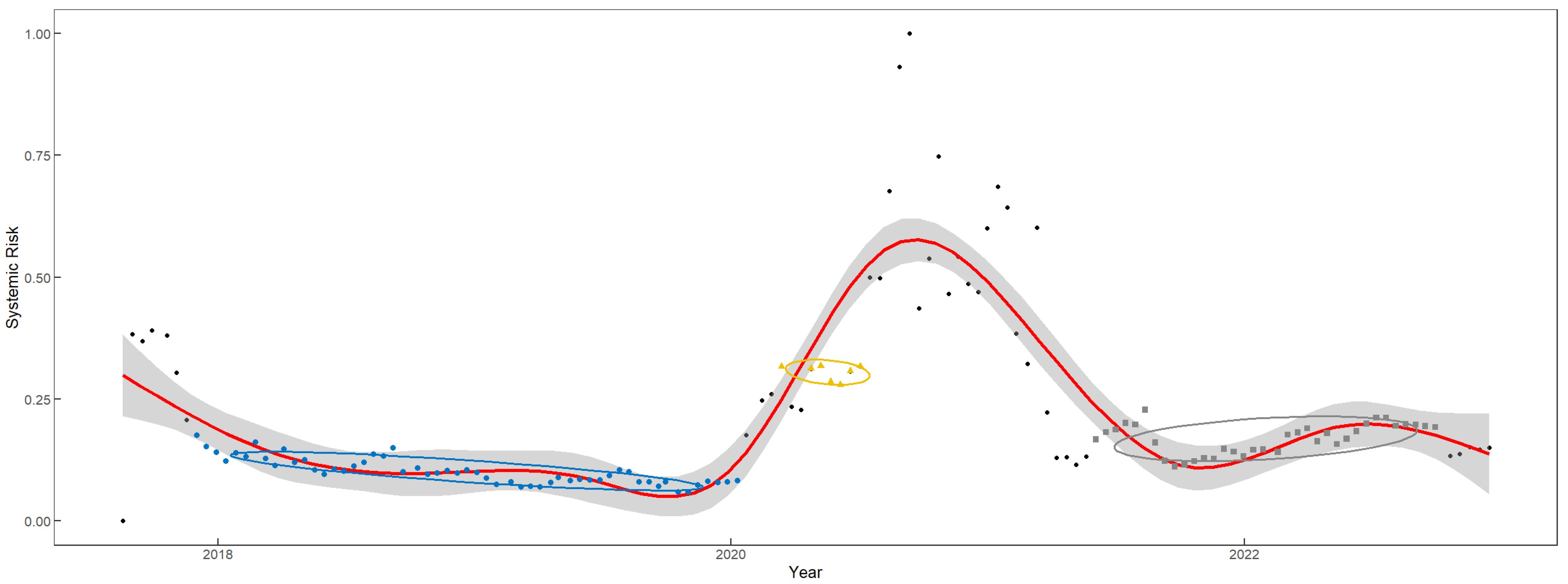
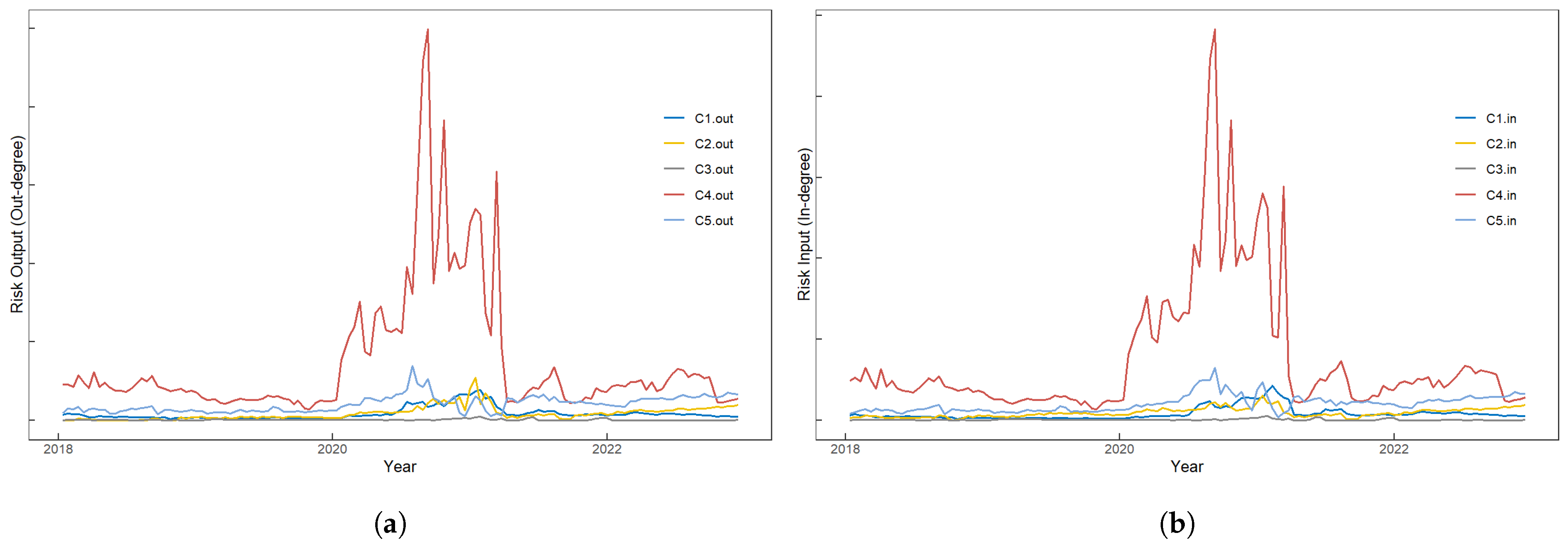
3.2.5. Systemic Risk over Time
3.2.6. Dynamics of Systemic Risk Structures in Chinese Stock Market
4. Discussion
4.1. Conclusions
- By analyzing the four conventional network metrics—in-degree, out-degree, closeness centrality, and betweenness centrality—insurance companies serve both as the main contributors and major receivers of the systemic risk in the Chinese stock. No single stock significantly influences the others, but companies like Hang Seng Electronics play a pivotal role in risk propagation.
- By analyzing the main risk output and input centers obtained from the HITS algorithm, we find that the biggest risk output centers are PingAn, CPIC and NCI; the biggest risk input centers are CLIC and NCI.
- By examining the temporal evolution of systemic risk in the Chinese stock market, we conclude that a pre-2020 period is characterized by relatively low systemic risk. However, the onset of the COVID-19 pandemic’s initial wave instigates significant shifts. Stringent pandemic control measures precipitate disruptions in the supply chain, production halts in select industries, and a pervasive sense of market tension, thereby engendering a noteworthy upsurge in systemic risk within the Chinese stock market. After the implementation of effective COVID-19 control measures, systemic risk reverts to normal levels in early 2021.
- Moreover, an exploration of community characteristics derived from a community detection algorithm underscores that the sources of risk in the Chinese stock market from 2018 to 2022 predominantly manifest within sectors such as the secondary industry, emerging industries, and insurance. Each of these categories exhibits a pronounced internal correlation. The classification approach employed herein primarily hinges on the interplay of risk among companies, differing from conventional categorizations such as insurance, financial services, and others. Within this framework, the principal sources of risk emanate from the insurance sector. It is plausible that events such as pandemics can induce systemic risk in the insurance industry, and as these entities engage in non-traditional business activities, such endeavors may further contribute to systemic risks within the network.
4.2. Limitation and Further Work
Author Contributions
Funding
Institutional Review Board Statement
Informed Consent Statement
Data Availability Statement
Conflicts of Interest
Abbreviations
| ACF | Autocorrelation Function |
| ADF | Augmented Dickey–Fuller |
| CLIC | China Life Insurance Company Ltd. |
| CNPC | PetroChina Company Ltd. |
| CPIC | China Pacific Insurance Company Ltd. |
| CoES | Conditional Expected Shortfall |
| CoVaR | Conditional Value at Risk |
| DBSCAN | Density-Based Spatial Clustering of Applications with Noise |
| ES | Expected Shortfall |
| HITS | Hyperlink-Induced Topic Search |
| MES | Marginal Expected Shortfall |
| NCI | Xinhua Insurance |
| RTI | Risk Transmission Index |
| PACF | Partial Autocorrelation Function |
| PingAn | Ping An Insurance |
| SCAD | Smoothly Clipped Absolute Deviation |
| SES | Systemic Expected Shortfall |
| SIFI | Systemic Important Financial Institution |
| SZ180 | Shanghai 180 Index |
| VaR | Value at Risk |
| 1 | Ping An Bank is listed on the Shenzhen Stock Exchange, so we didn’t include it in our research. |
References
- Acharya, Viral V., Lasse H. Pedersen, Thomas Philippon, and Matthew Richardson. 2017. Measuring systemic risk. The Review of Financial Studies 30: 2–47. [Google Scholar] [CrossRef]
- Artzner, Philippe, Freddy Delbaen, Jean-Marc Eber, and David Heath. 1999. Coherent measures of risk. Mathematical Finance 9: 203–28. [Google Scholar] [CrossRef]
- Blondel, Vincent D., Jean-Loup Guillaume, Renaud Lambiotte, and Etienne Lefebvre. 2008. Fast unfolding of communities in large networks. Journal of Statistical Mechanics: Theory and Experiment 10: 10008. [Google Scholar] [CrossRef]
- Bo, Lin, and Zheng Li. 2016. Research on the Measurement and Monitoring of Systemic Risk in Finance. Nankai Journal: Philosophy, Social Sciences Edition 4: 150–60. [Google Scholar]
- Brownlees, Christian, and Robert F. Engle. 2017. SRISK: A conditional capital shortfall measure of systemic risk. The Review of Financial Studies 1: 48–79. [Google Scholar] [CrossRef]
- Diebold, Francis X., and Kamil Yılma. 2014. On the network topology of variance decompositions: Measuring the connectedness of financial firms. Journal of Econometrics 182: 119–34. [Google Scholar] [CrossRef]
- Duffie, Darrell, and Jun Pan. 1997. An overview of value at risk. Journal of Derivatives 4: 7–49. [Google Scholar] [CrossRef]
- Ester, Martin, Hans-Peter Kriegel, Jörg Sander, and Xiaowei Xu. 1996. A density-based algorithm for discovering clusters in large spatial databases with noise. In kdd. München: Institute for Computer Science, University of Munich, Oregon: AAAI Press, vol. 96, pp. 226–31. [Google Scholar]
- Fan, Jianqing, and Runze Li. 2001. Variable selection via nonconcave penalized likelihood and its oracle properties. Journal of the American Statistical Association 96: 1348–60. [Google Scholar] [CrossRef]
- Fang, Yi, Shengmin Zhao, and Daoping Wang. 2012. Measurement of Systemic Risk in China’s Financial Institutions: A Study Based on the DGC-GARCH Model. Financial Regulation Research 11: 26–42. [Google Scholar]
- Hautsch, Nikolaus, Julia Schaumburg, and Melanie Schienle. 2015. Financial network systemic risk contributions. Review of Finance 19: 685–738. [Google Scholar] [CrossRef]
- Härdle, Wolfgang Karl, Weining Wang, and Lining Yu. 2016. Tenet: Tail-event driven network risk. Journal of Econometrics 192: 499–513. [Google Scholar] [CrossRef]
- Kaufman, George G., and Kenneth E. Scot. 2003. What is systemic risk, and do bank regulators retard or contribute to it? The Independent Review 7: 371–91. [Google Scholar]
- Kleinberg, Jon M. 1999. Authoritative sources in a hyperlinked environment. Journal of the ACM (JACM) 46: 604–32. [Google Scholar] [CrossRef]
- Kupiec, Paul H. 1995. Techniques for Verifying the Accuracy of Risk Measurement Models. Washington, DC: Division of Research and Statistics, Division of Monetary Affairs, Federal Reserve Board, vol. 95, pp. 73–84. [Google Scholar]
- Lai, Juan. 2011. Research on Systemic Risk in China’s Finance and Its Prevention. Doctoral dissertation, Jiangxi University of Finance and Economics, Nanchang, China. [Google Scholar]
- Li, Zhihui, Yuan Li, and Zheng Li. 2016. Research on Monitoring Systemic Risk in China’s Banking Industry: Implementation and Optimization Based on SCCA Technology. Financial Research 429: 92–106. [Google Scholar]
- Lin, Yuanlong. 2023. The Impact of the COVID-19 Pandemic on the Chinese Stock Market. Master’s thesis, Jilin University, Jilin, China. [Google Scholar]
- Tobias, Adrian, and Markus K. Brunnermeier. 2016. CoVaR. The American Economic Review 106: 1705. [Google Scholar]
- Wu, Qingwei, Tao Hong, and Jun Ma. 2010. A Review of the Long Tail Theory. Journal of Zhoukou Normal University 27: 124–29. [Google Scholar]
- Zhang, Yuanping, and Gang Sun. 2003. Theoretical Analysis and Empirical Study on Financial Crisis Early Warning System. International Financial Research 10: 32–38. [Google Scholar]


| Macroeconomic Indicators | Frequency | Category | Stationarity Transformation |
|---|---|---|---|
| Export Value (Current value) | Monthly | Foreign Trade Indicators | Log 1st Difference |
| Import Value (Current value) | Monthly | Log 1st Difference | |
| Real Estate Development Composite Prosperity Index (Current value) | Monthly | Real Estate Related Indicators | 1st Difference |
| Fixed Asset Investment Completed Value (Accumulated YoY) | Monthly | 1st Difference | |
| Real Estate Development Investment Completed Value (Accumulated value) | Monthly | 12th Difference | |
| Total Retail Sales of Consumer Goods (Current YoY) | Monthly | Consumer Related Indicators | 1st Difference |
| Consumer Price Index (CPI) (Current YoY) | Monthly | None | |
| Consumer Confidence Index (Current value) | Monthly | 1st Difference | |
| Per Capita Disposable Income of Urban Residents (Accumulated value) | Quarterly | 4th Difference | |
| Per Capita Consumption Expenditure of Urban Residents (Accumulated value) | Quarterly | 4th Difference | |
| Value Added of Wholesale and Retail Trade (Current YoY) | Quarterly | 4th Difference | |
| Electricity Generation Output (Accumulated value) | Monthly | Energy Logistics Related Indicators | 12th Difference |
| Total Freight Volume (Accumulated value) | Monthly | 12th Difference and 1st Difference | |
| Railway Freight Volume (Accumulated YoY) | Monthly | 1st Difference | |
| Purchasing Price Indices of Raw Material (PPIRM) (Current value) | Monthly | Commodity Related Indicators | 1st Difference |
| Retail Price Index (RPI) (Current YoY) | Monthly | 1st Difference | |
| Producer Price Index (PPI) (Current YoY) | Monthly | 1st Difference | |
| Corporate Goods Price Index (CGPI) (Current YoY) | Monthly | 1st Difference | |
| China Commodity Price Index (Current value) | Monthly | 1st Difference | |
| Money & Quasi-money(M2) | Monthly | 1st Difference | |
| Interbank Repo Benchmark Interest Rate (Current value) | Daily | Financial Market Indicators | 1st Difference |
| Weighted Average Overnight Interbank Borrowing Rate (Current value) | Monthly | 1st Difference | |
| China Government Bond Yield (10-year) | Monthly | 1st Difference | |
| Total Outstanding Loans of Financial Institutions (Domestic and Foreign Currency) (Current YoY) | Monthly | 1st Difference | |
| Total Social Financing Scale (Stock) (Current YoY) | Monthly | 1st Difference | |
| Keqiang Index (Accumulated value) | Monthly | Macroeconomic Overall Indicators | 1st Difference |
| Gross Domestic Product (GDP) (Current value) | Quarterly | Log 1st Difference | |
| Value Added of the Primary Industry (Current value) | Quarterly | 4th Difference | |
| Value Added of the Secondary Industry (Current value) | Quarterly | 4th Difference | |
| Value Added of the Tertiary Industry (Current value) | Quarterly | 4th Difference |
| Model | 25% Quantile of Proportion Exceeding Estimated VaR | 75% Quantile of Proportion Exceeding Estimated VaR | Proportion Passing Backtesting (0.05) |
|---|---|---|---|
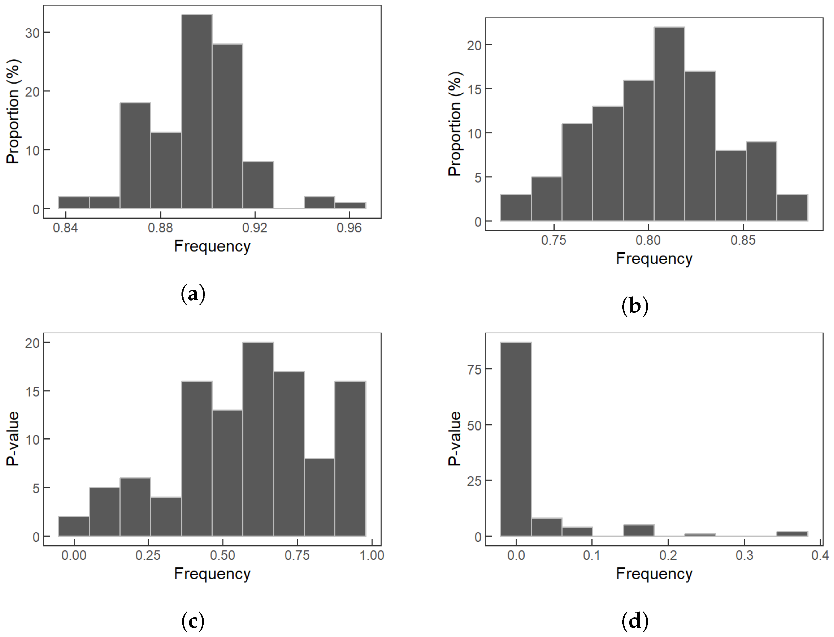
| QR–Lasso Model | 0.88 | 0.91 | 98.1% |
| Quantile Regression Model | 0.78 | 0.82 | 14.0% |
| Indicator | Definition | Interpretation |
|---|---|---|
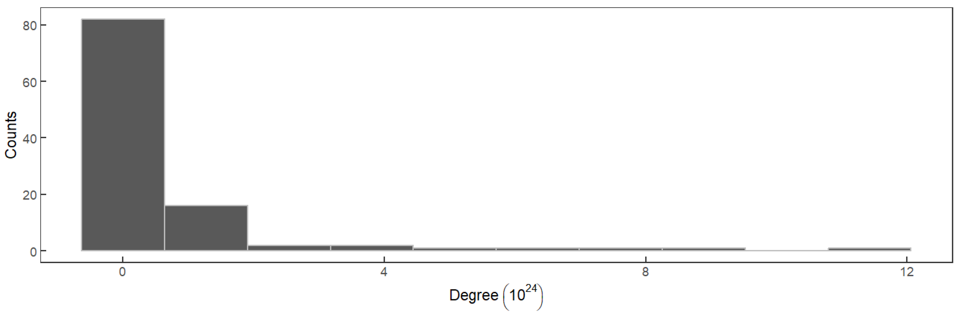
| Degree | Judge if the network follows a power-law distribution | |
| In-degree | Total systemic risk transmitted by individual stocks | |
| Out-degree | Total systemic risk received by individual stocks | |
| Closeness Centrality | where is the shortest path from i to j | Indicates whether a stock has a dominant role in other stocks’ CoVaR |
| Betweenness Centrality | where calculates if i lies on the shortest path between s and v | Measures a stock’s ability to propagate risk within the system |
Disclaimer/Publisher’s Note: The statements, opinions and data contained in all publications are solely those of the individual author(s) and contributor(s) and not of MDPI and/or the editor(s). MDPI and/or the editor(s) disclaim responsibility for any injury to people or property resulting from any ideas, methods, instructions or products referred to in the content. |
© 2024 by the authors. Licensee MDPI, Basel, Switzerland. This article is an open access article distributed under the terms and conditions of the Creative Commons Attribution (CC BY) license (https://creativecommons.org/licenses/by/4.0/).
Share and Cite
Zeng, X.; Hu, Y.; Pan, C.; Hou, Y. Exploring Systemic Risk Dynamics in the Chinese Stock Market: A Network Analysis with Risk Transmission Index. Risks 2024, 12, 56. https://doi.org/10.3390/risks12030056
Zeng X, Hu Y, Pan C, Hou Y. Exploring Systemic Risk Dynamics in the Chinese Stock Market: A Network Analysis with Risk Transmission Index. Risks. 2024; 12(3):56. https://doi.org/10.3390/risks12030056
Chicago/Turabian StyleZeng, Xiaowei, Yifan Hu, Chengjun Pan, and Yanxi Hou. 2024. "Exploring Systemic Risk Dynamics in the Chinese Stock Market: A Network Analysis with Risk Transmission Index" Risks 12, no. 3: 56. https://doi.org/10.3390/risks12030056