
Adding Shocks to a Prospective Mortality Model


1
Prim’Act, 75017 Paris, France
2
ISFA, Institut de Science Financière et d’Assurances (ISFA), Laboratoire SAF EA2429, Université de Lyon, Université Claude Bernard Lyon 1, 69366 Lyon, France
*
Author to whom correspondence should be addressed.
Risks 2024, 12(3), 57; https://doi.org/10.3390/risks12030057
Submission received: 2 January 2024
/
Revised: 12 March 2024
/
Accepted: 15 March 2024
/
Published: 20 March 2024
(This article belongs to the Special Issue Advancement in Mortality Forecasting and Mortality/Longevity Risk Management)
Abstract
:This work proposes a simple model to take into account the annual volatility of the mortality level observed on the scale of a country like France in the construction of prospective mortality tables. By assigning a frailty factor to a basic hazard function, we generalise the Lee–Carter model. The impact on prospective life expectancies and capital requirements in the context of a life annuity scheme is analysed in detail.
1. Introduction
The construction of life expectancy projections has been the subject of many works since the seminal article by Lee and Carter (Lee and Carter 1992).
For the purpose of extrapolating trends observed in the past into the future, most of the approaches that have been proposed are based on a “mortality surface”, which measures mortality forces by age and year at a given time, and smoothly extrapolates these into the future.
The models inspired by Lee and Carter start by reducing dimensions by performing a PCA and then extrapolating one or two time series associated with the projection on the principal axes (see Plat 2009 for a detailed discussion).
Bongaarts (Bongaarts 2004) proposed a different approach, based on parametric adjustments by year of time vs. year of age and extrapolation of the estimated coefficients each year.
In Bongaarts (2004), however, the author uses a rather simple parametric representation (Thatcher’s model, see Thatcher 1999), which does not allow all ages to be included. Moreover, he limits his extrapolation to two out of three parameters (the age structure of the mortality is assumed to be independent of time), treating them independently, which is a questionable approximation (time varying coefficients for accident and aging should be dependent).
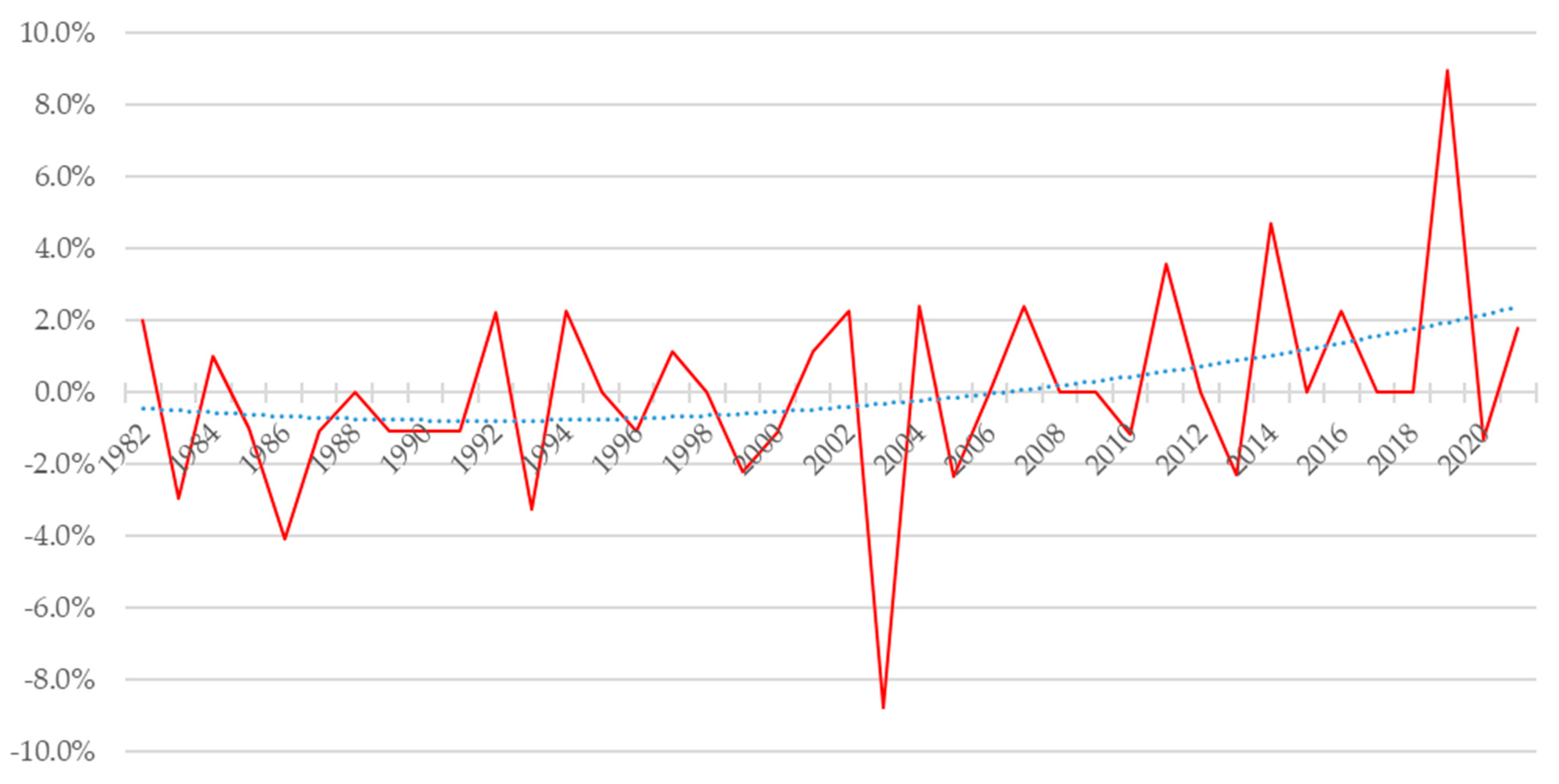
This type of model projects a smooth series. Given and the risk exposures , we compute the annual global mortality rate in France, . When looking at annual variations in this mortality rate from 1982 to 2022 (see Figure 1), we see a rather high degree of volatility. On this figure, the red line is the annual variation of mortality, whereas the blue line is a quadratic fit of this annual variation.
The classic models described above cannot easily account for these short-term variations. The “probabilistic version” of the Lee–Carter model proposed by Brouhns et al. (2002) could be used as a stochastic mortality model, but at the cost of being somewhat cumbersome to implement. What is more, the uncertainty included in this model refers solely to the estimation risk, whereas here we are seeking to account for a different kind of uncertainty, relating to the underlying mortality itself. Proposed approaches for this have been put forward, for example, in Guette (2010) or Currie et al. (2003), but with a slightly different objective, as these works propose to model catastrophes (rare high-intensity events) such as wars or severe epidemics. More recently, an approach using regime-switching models was proposed in Robben and Antonio (2023).
However, our aim here is not to model rare events, but to incorporate the above volatility into the model, in order to provide a more accurate assessment of residual life expectancies when an unbiased estimate of mortality rates is available. We are not concerned here with trend risk, for which there are many models (see Juillard et al. 2008; Juillard and Planchet 2006; Plat 2009), but only with the short-term shift in mortality trend.
Therefore, a specific approach is proposed here, with the aim of accounting for this short-term volatility and measuring its impact on the anticipation of prospective residual life expectancies in a parsimonious way.
We draw inspiration here from the frailty models proposed by Vaupel and his co-authors (Vaupel et al. 1979) by applying to a regular base hazard function a shock that depends only on time, under a proportional hazards assumption. This model was generalised by Barbi (1999), who proposed a heterogeneity model called “combined fragility”, still assuming proportional fragility initially distributed according to a Gamma distribution. It is used in Barbi et al. (2003), for example, to study the extreme age of survival.
Very recently, Carannante et al. (2023) offered a frailty version of the Lee–Carter model which is very close to ours.
The frailty factor is not used here to consider population heterogeneity, as is usually the case, but to introduce uncertainty into the model’s basic hazard function. The frailty factor is thus designed to account for annual shifts around a steady mortality trend.
For further references, reader may look at (Debonneuil 2015; Guilbaud 2018; Planchet and Thérond 2011).
2. Proposed Stochastic Mortality Model
The proposed specification is described below, followed by a method for estimating the parameters within the framework of conditional maximum likelihood.
2.1. Specification
Consider the following specification of the (stochastic) hazard function for the year of time t:
with the semi-parametric form of the basic hazard function . The shocks at time are introduced through the random variable These shocks are assumed to be independent, identically distributed and mean-centred, i.e., . Because is assumed to be deterministic, this model differs from the one described in Plat (2009). What is more, in his article, Plat proposes interesting ways to model uncertainty about the mortality trend. Here, we are interested in short-term deviations in the level of mortality, with all ages combined. The two approaches are, therefore, complementary and do not consider the same risks.
We use the usual identifiability conditions for the basic hazard function, which are imposed1 as follows (cf. Brouhns et al. 2002):
and
This involves estimating the parameters of and the matrix , then extrapolating the time series .
2.2. Log-Likelihood Determination
For maximum likelihood estimation, we know that everything happens as if the number of deaths observed followed a Poisson distribution,
which leads to the following expression for the conditional likelihood for an observation, noting and :
Likelihood for one observation is easy to obtain:
We then choose a Gamma distribution of parameters a and b for the distribution of , i.e., , which leads to
Using the change of variable , we obtain the following expression for the likelihood of an observation
which gives
which in turn gives log-likelihood
with .
As a function of the parameters and conditional on , the log-likelihood for an observation is of the form with . Conditional on , the log-likelihood has the following form (with one additive constant):
which gives
Ultimately, this model aims to study the extent to which short-term volatility of mortality rates may impact prospective mortality rates. It is accomplished through the presence of parameters and in the log-likelihood, which can then be maximised by under the constraint given by Equations (2) and (3). This task is performed in the next section.
2.3. Parameter Estimation
Parameter estimation can be carried out in two stages: in the first stage, the frailty parameter is estimated, then, in the second stage, the above log-likelihood is maximised at .
The condition implies . We also have , so the disturbance control parameter is the inverse of the variance . A direct estimate of this parameter can be made as follows, observing that the mean annual output intensities are of the form
with
from which we derive , then . That last equation is equivalent to , with being the coefficient of variation of and being the standard deviation of .
It is then straightforward to use the usual estimator for :
with and corresponding to the Hoem estimator of the hazard function:
and
Given that and using Equation (15), the frailty parameter can be estimated as follows:
Once the frailty parameter has been estimated, the aim is to maximise the previously expressed log-likelihood. The partial derivatives of the log-likelihood for an observation are as follows:
with p one of the parameters . Since
and
it is possible to estimate , as a solution of the following first-order conditions:
This system is non-linear.
2.4. Calculating Prospective Residual Life Expectancies
In the proposed model, the calculation of prospective life expectancy proceeds as follows
Given the linearity of expectancy in a finite sum and knowing that the shocks are assumed to be independent, the prospective life expectancy takes the form
We then have
because the Laplace transform of a Gamma distribution is . As , we deduce that:
Note that and then we find the classic formula
3. Numerical Application
We use data for metropolitan France for the period of 2000 to 2020, with ages 0 to 105 included, from the Agalva and Blanpain (2021) study. The choice of these data is motivated by the desire to be consistent with the work of estimating future mortality of INSEE, which provided us with the data. The year 2020, which sees a significant increase in mortality compared to 2019 (which was, on the contrary, a year of particularly low mortality), is logically included in the study, as it is one of the non-catastrophic events (in the sense defined above) that we want to include in the modelling.
All calibration was performed in R 4.3.1.
Prospective analyses are then carried out over the entire age range and for the years of 2021 to 2060, to enable comparisons to prospective tables compiled by INSEE.
3.1. Model Adjustment
All of these steps are discussed in turn in the following subsections. Throughout the study, all of the results obtained are compared to those given by a Lee–Carter model calibrated on the same data.
3.1.1. Estimation of Gamma Distribution Parameters
The estimation of the pair of parameters has been made with the raw data, and we find that , i.e., .
3.1.2. Estimation of Model Parameters
The calibration of under constraints was then carried out using the2 Rsolnp package, and more specifically the solnp function (see Ghalanos and Theussl 2015). This function is based on the solver by Yinyu Ye (see Ye 1987).
In order to carry out this calibration, the results of a Lee–Carter model were chosen as initial parameters, calibrated using the lca function from the3 demography package (see Hyndman 2023). All of these coefficients are transcribed in Appendix A.
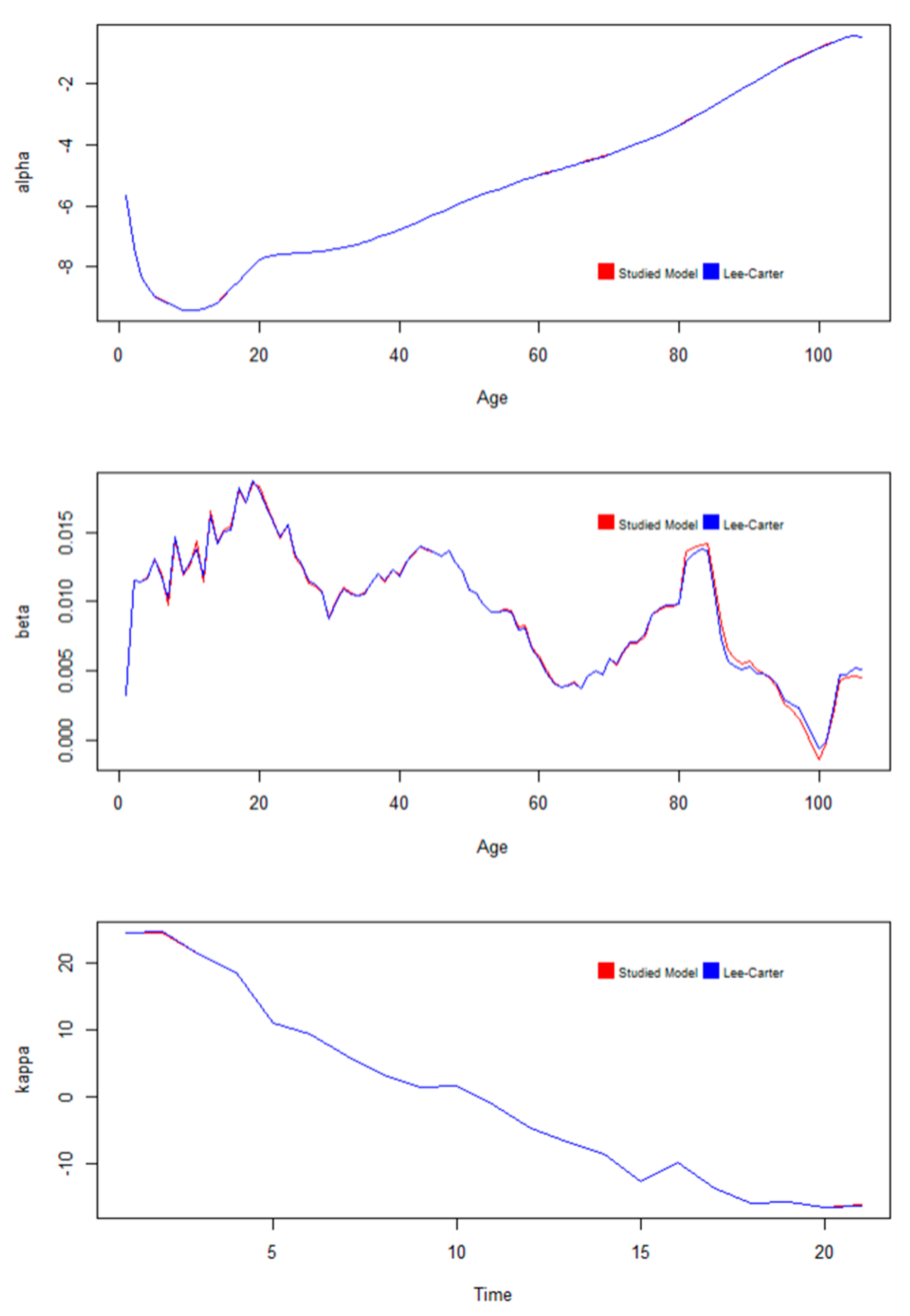
As shown in the following figure (Figure 2), this leads to coefficients that are very close to those of the referenced Lee–Carter model:
It can be seen that the time parameter shows a slower rate of decline from the 18th year of the observation period.
3.1.3. Extrapolation of Time Coefficients
Whether in the model studied here or in the Lee–Carter model used as a reference, the projection of coefficients for beyond the calibration range have been performed by linear regression, by fitting the following equation to the calibrated parameters:
In both cases, we find the coefficients shown in the following table (Table 1):
The results are logically very similar in both cases.
3.2. Projected Mortality Forces
Here, we compare projected mortality forces with and without shocks integrated into the model, as a function of age and year.
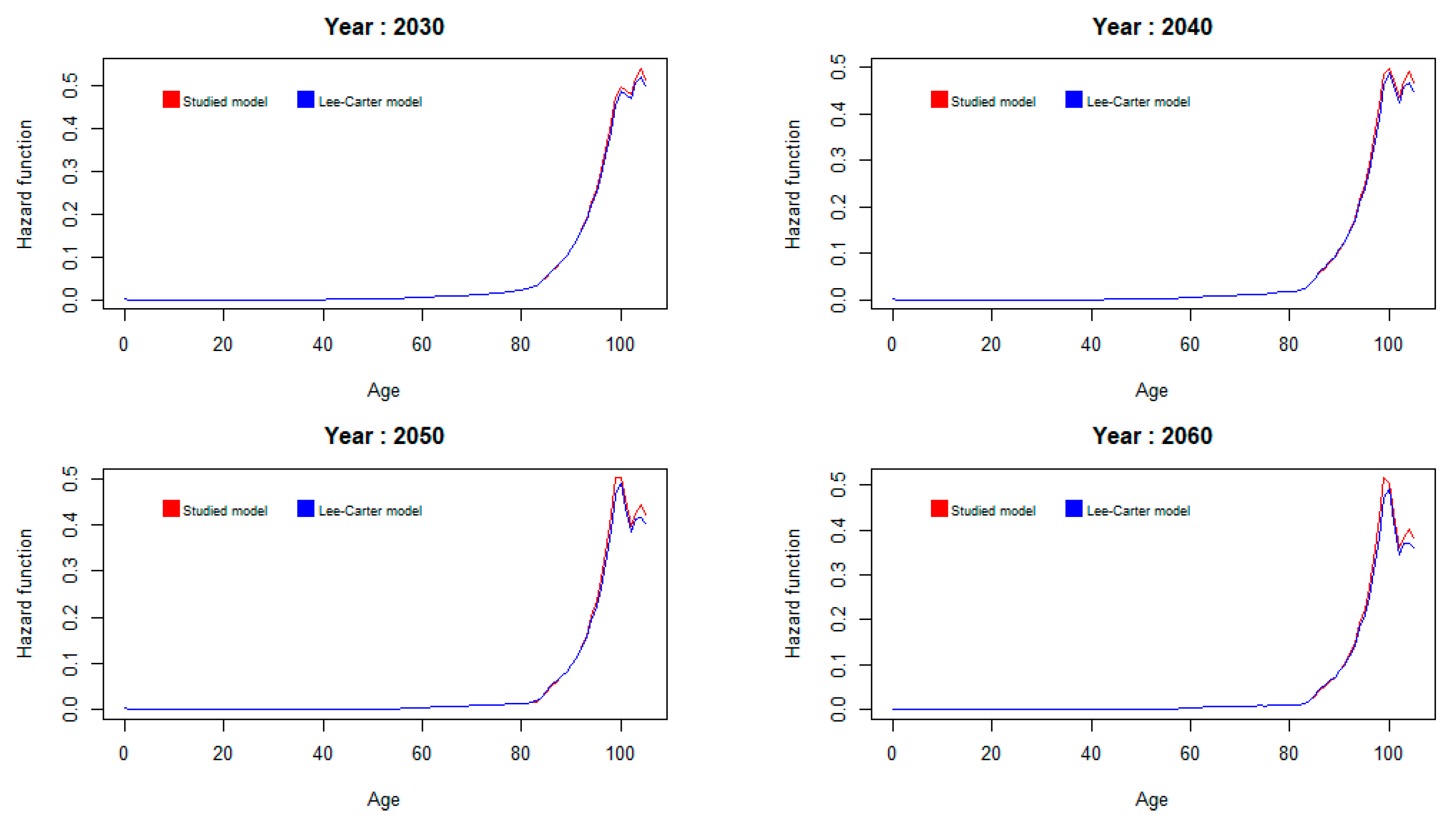
First, we look at the evolution of the mortality force as a function of age, for a few fixed years, as show in Figure 3:
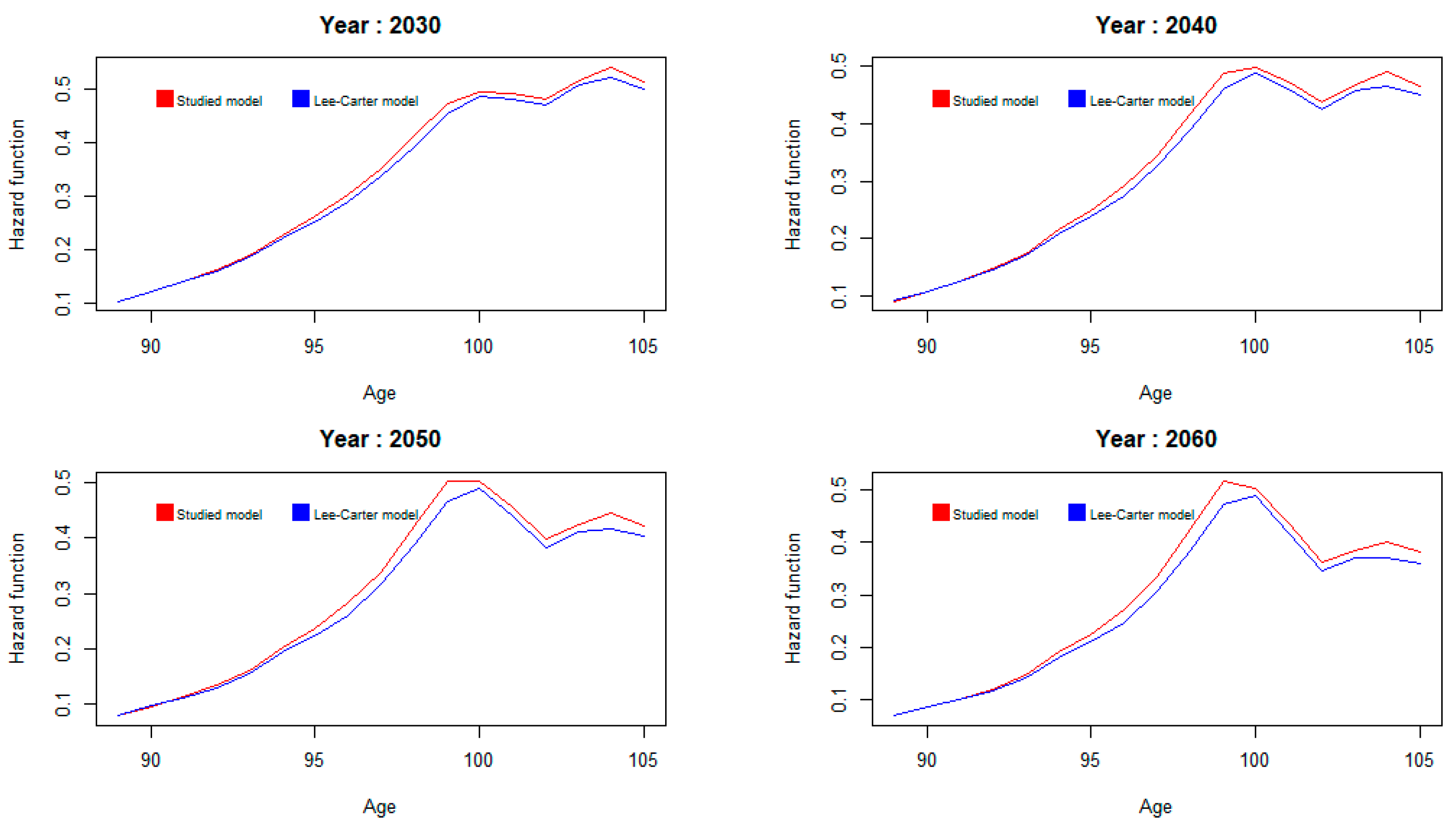
The mortality forces of the two models are very close, except at the highest ages, where the model with shocks tends to predict higher mortality forces. A closer look at the age range [90; 105] reveals the Figure 4:
The maximum relative deviation over the entire prospective range is 3.6% at age 80 for the year 2060.
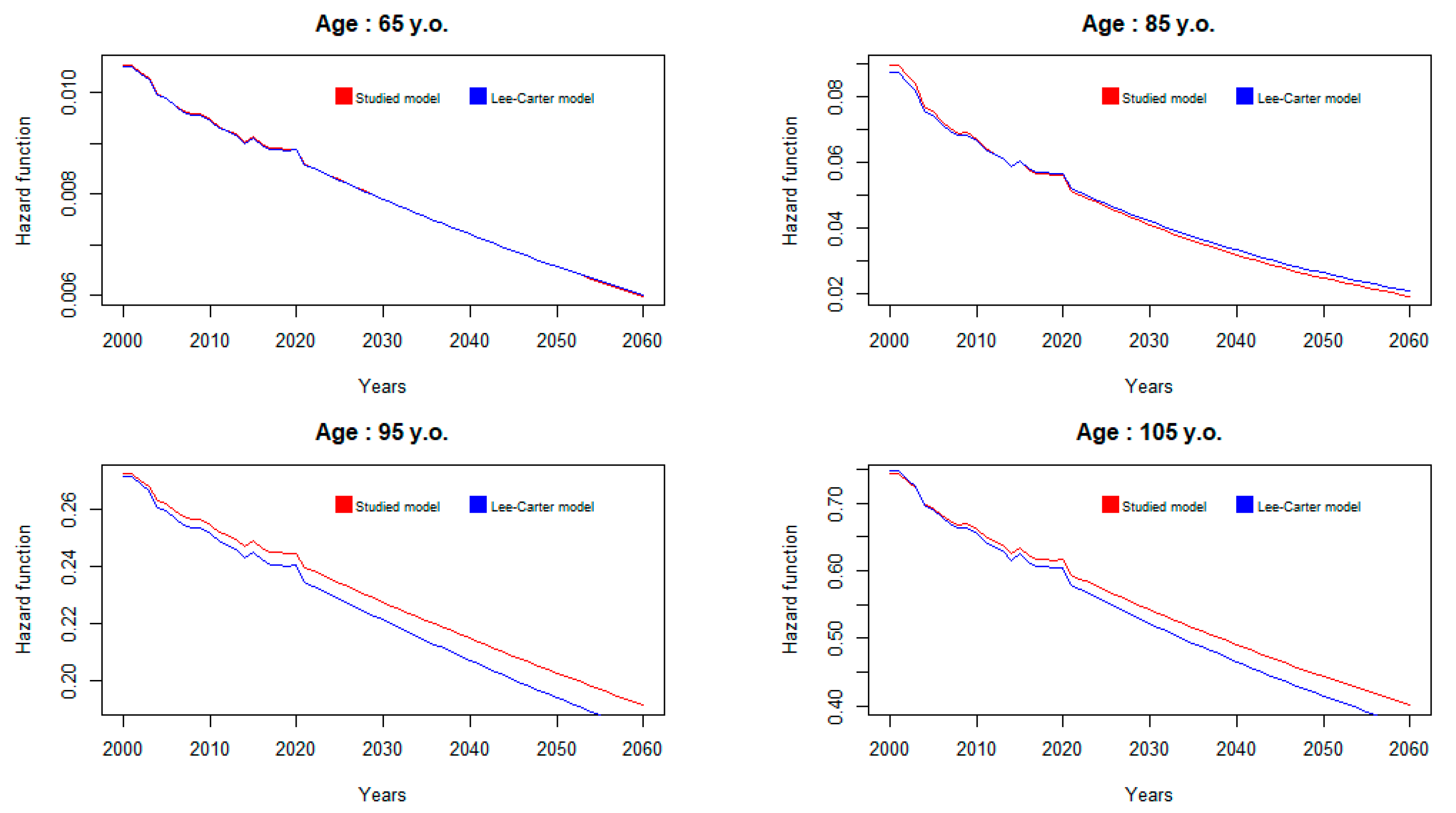
We now compare the mortality forces of the two models over the entire prospective analysis period, for a few selected ages. This comparison is performed in Figure 5:
Overall, the mortality model studied tends to predict higher mortality forces than the referenced Lee–Carter model at older ages, and the gap increases over time.
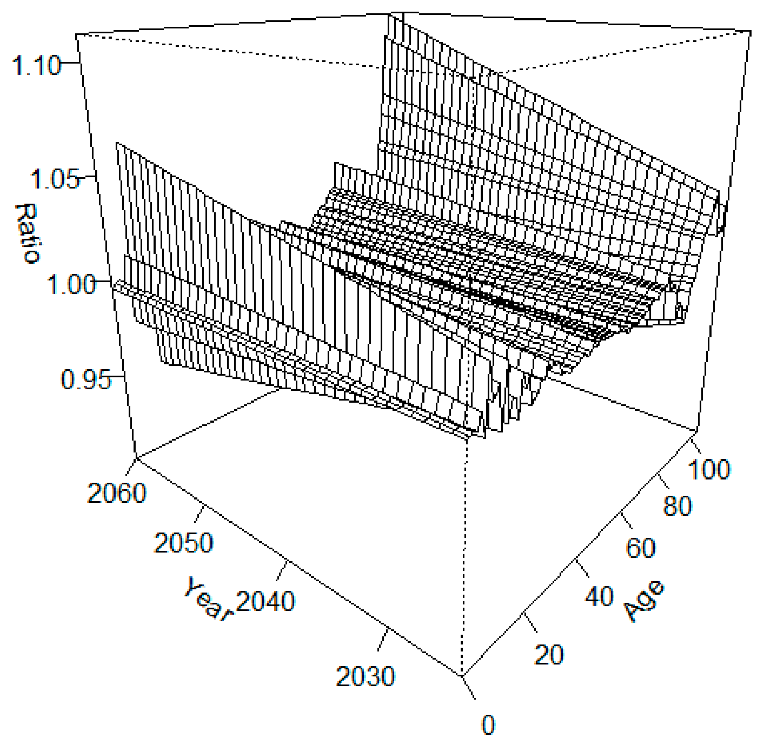
Before calculating prospective residual life expectancies, it is worth looking at the overall impact on mortality forces. To this end, we calculate the following ratio:
with , the mortality force derived from the referenced Lee–Carter model and model. This ratio is shown in the following figure (Figure 6):
The average value of this ratio for all ages and years combined is 100%, which means that the model studied is equivalent to the Lee–Carter model. This reflects the assumption made that the expectation of the frailty factor is equal to one.
The impact of the introduction of shocks on adjustment is, therefore, negligible when assessed on a very global basis. However, the difference increases over time, leading the two models to diverge in the medium term and at older ages.
If we restrict ourselves to ages over 65, we obtain a weighted average equal to 99.8%.
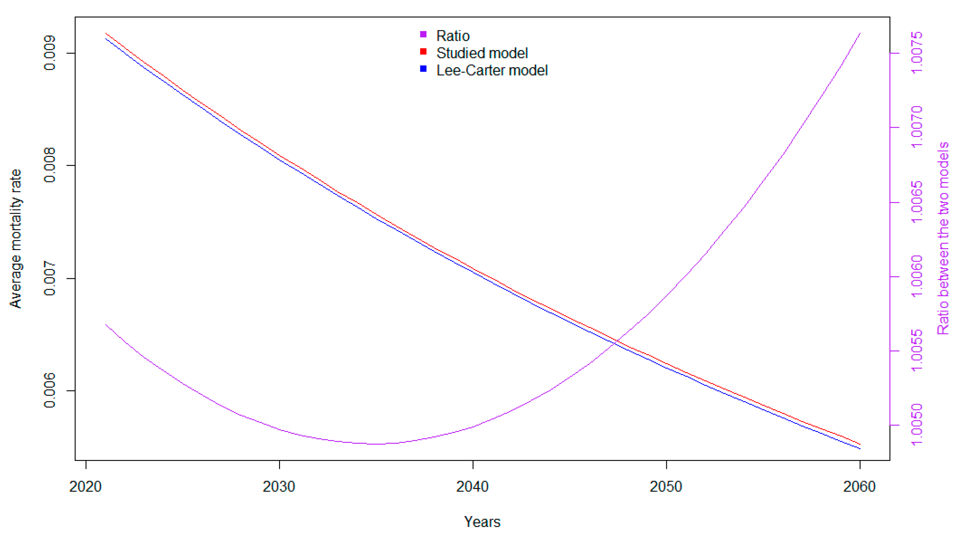
In addition, the average mortality rate of the population, calculated on the basis of exposure to risk in 2020, evolves as represented on Figure 7:
It can be seen that the model studied is on average more pessimistic than the Lee–Carter model on mortality improvement in future mortality, with a projected average mortality rate that is slightly higher than that derived from the Lee–Carter model.
3.3. Estimating Prospective Residual Life Expectancies
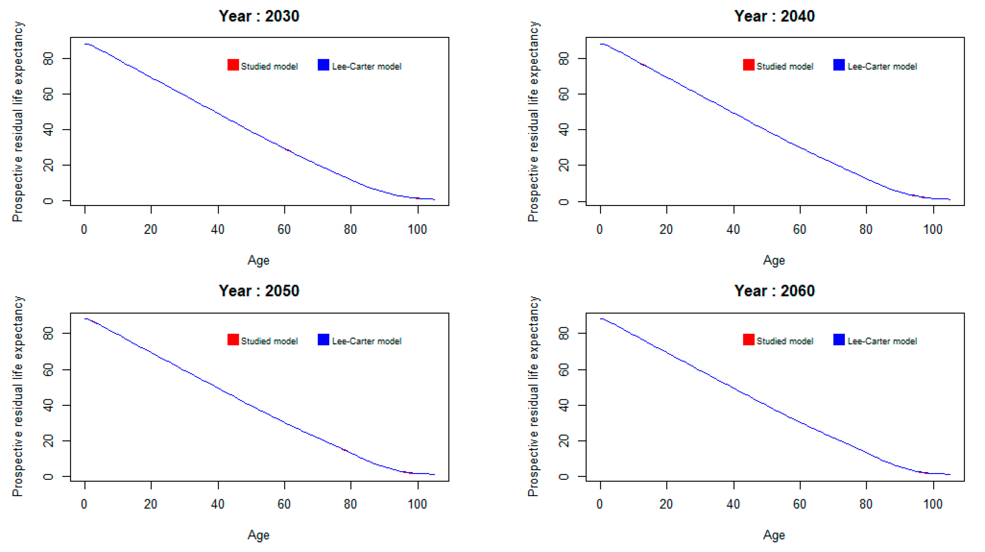
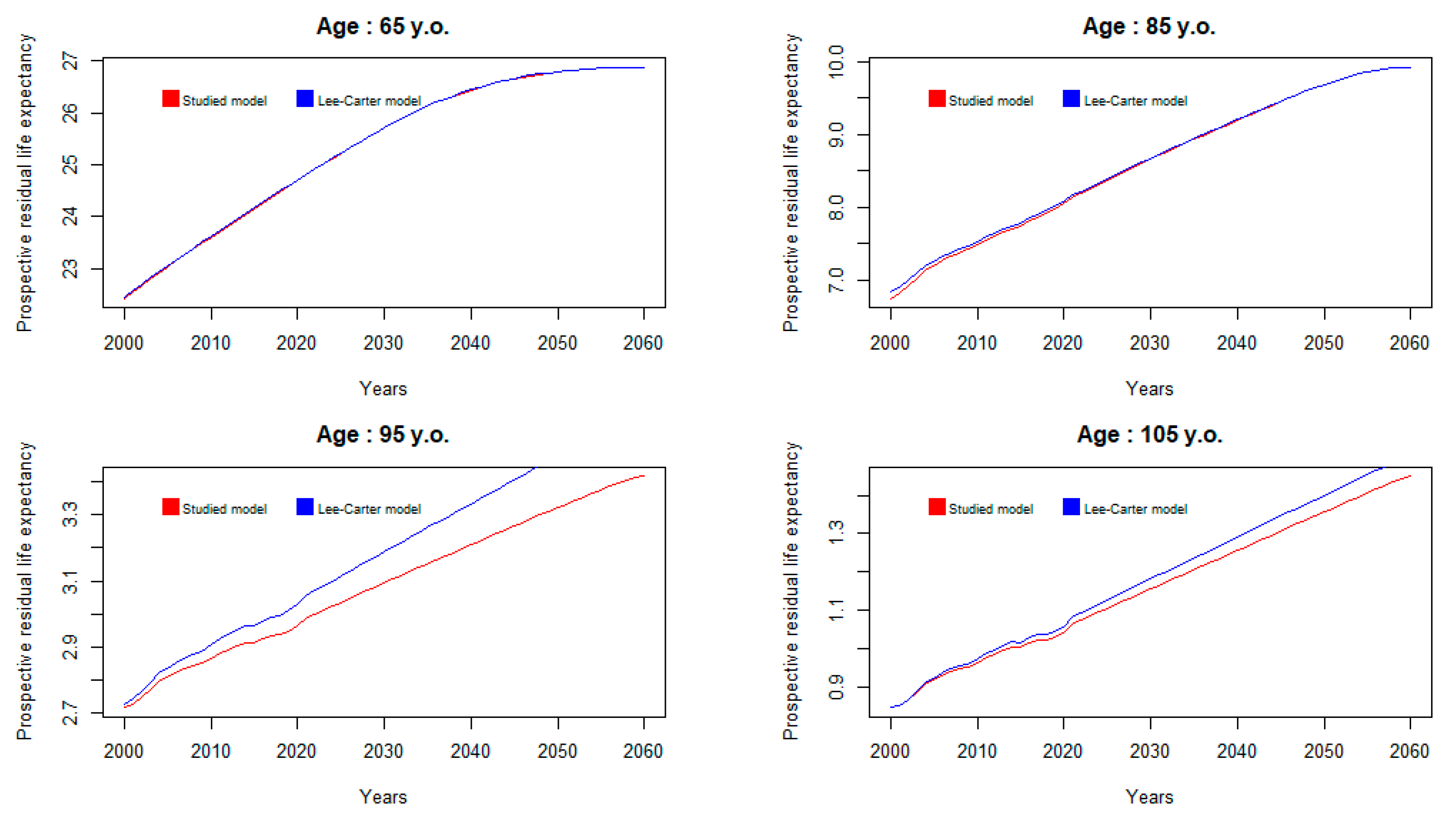
It is then possible to look at the consequences of the mortality model studied on prospective residual life expectancies, first by variable age for a few fixed years, then by variable year for a few fixed ages.
As shown in Figure 8, it appears that the mortality model studied does not greatly change prospective residual life expectancies compared to the reference mortality model, except possibly at high ages:
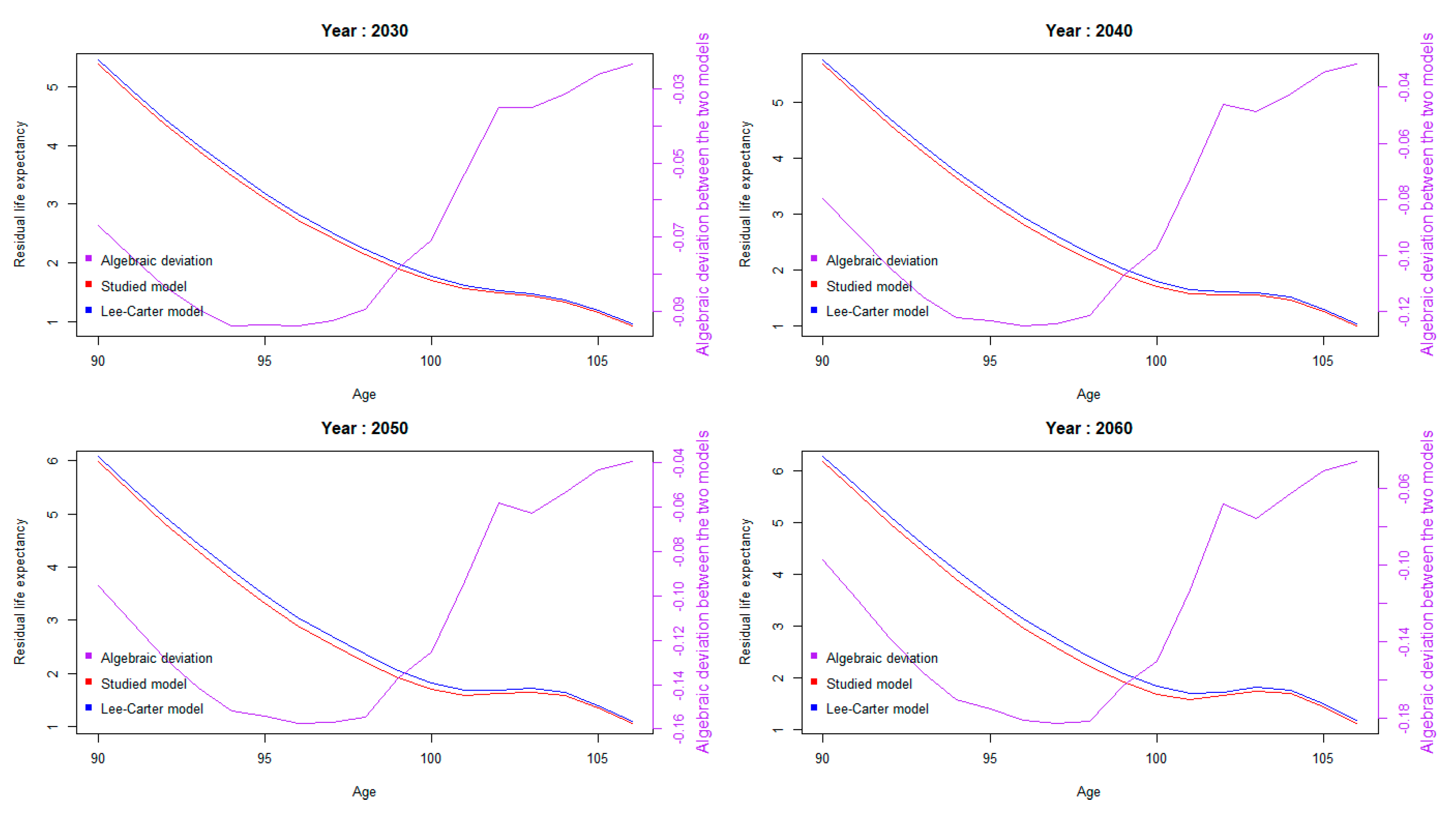
An enlargement of these graphs at older ages is shown below on Figure 9, with the algebraic difference between the two models for each year:
The maximum absolute difference between the two models is found at age 96 for the year 2060, and it is worth 0.18, or around 65 days.
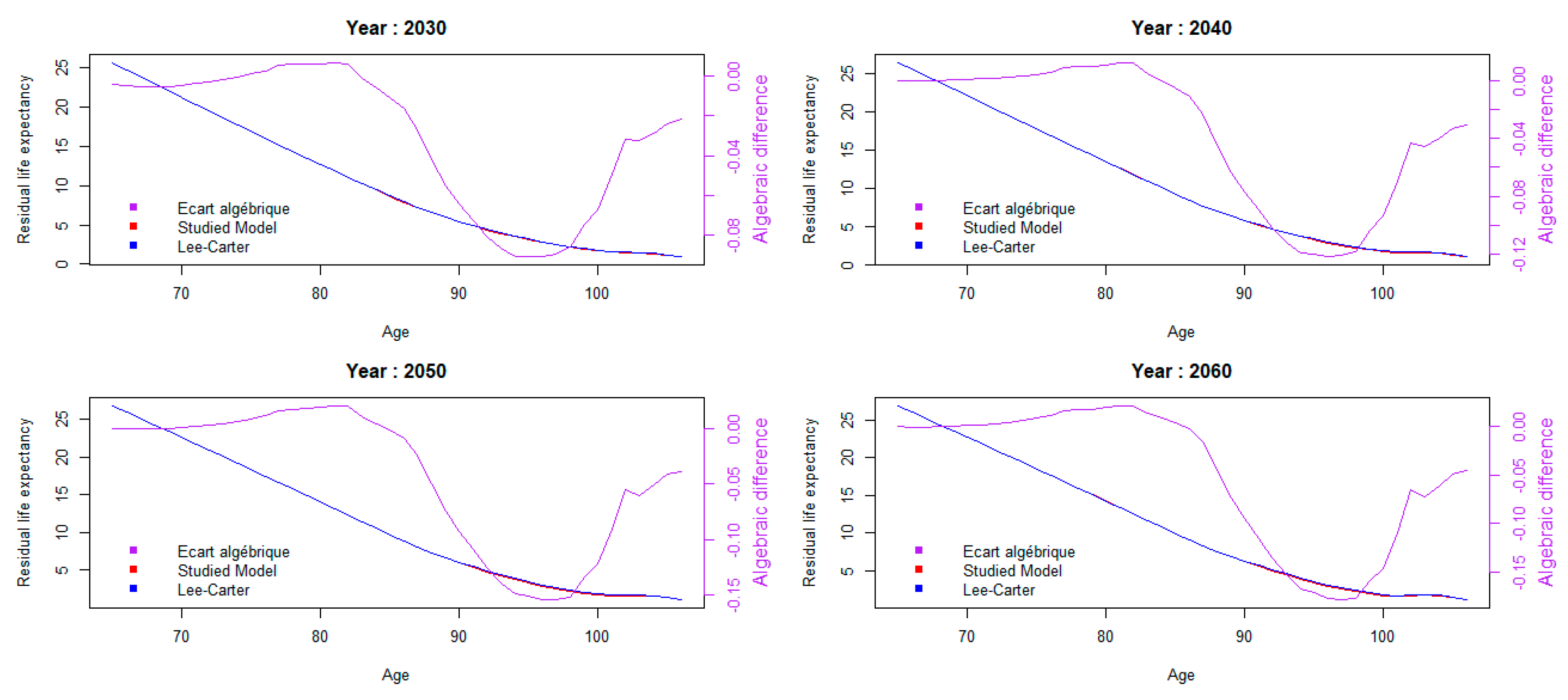
In this analysis, we return to the observation made in the previous section: he difference from the referenced Lee–Carter model is most marked for older ages, as shown on Figure 10.
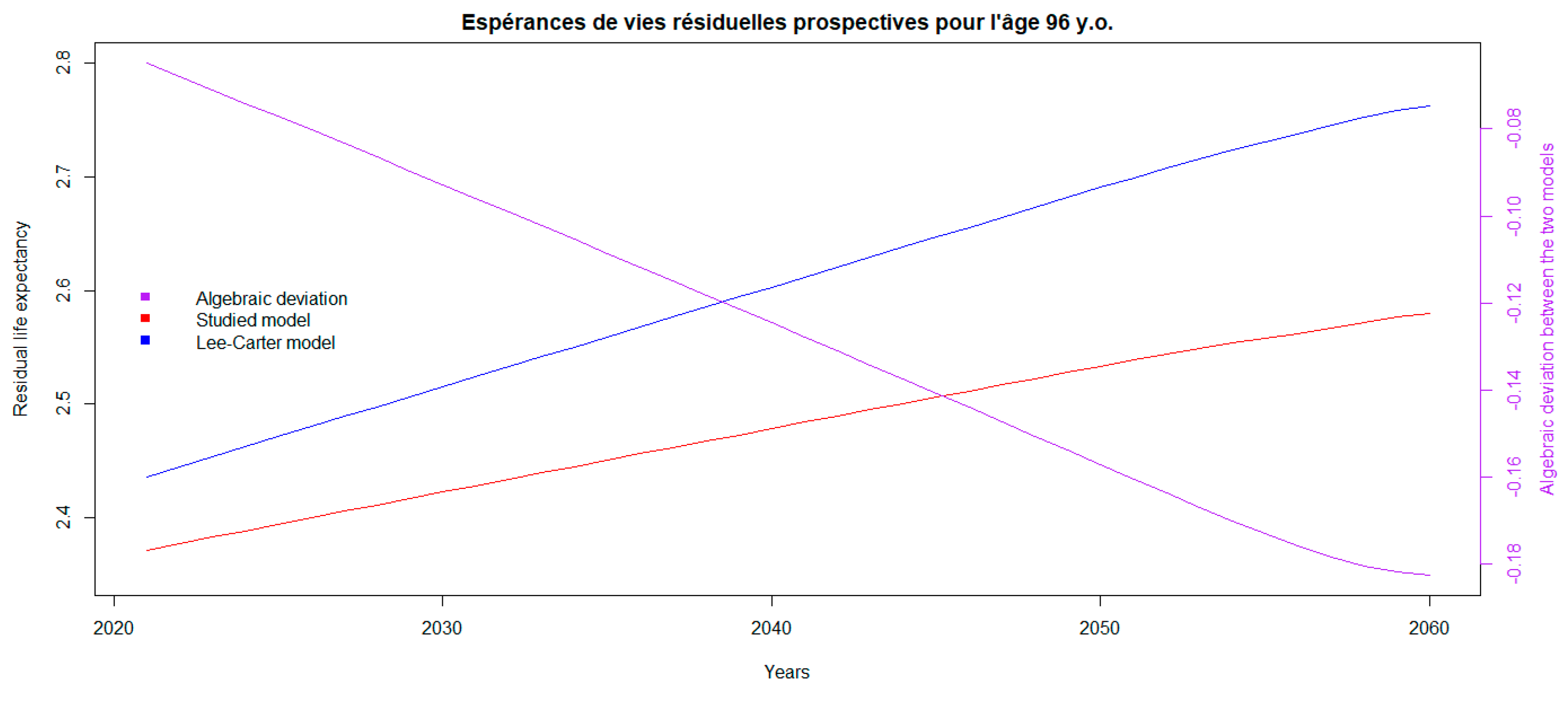
Below on Figure 11 is an enlargement for age 96 with the algebraic difference between the two models:
3.4. Sensitivity to Frailty Parameter
The volatility of frailty is estimated at 4.3%; however, over a longer period, this parameter can be higher. For example4, from 1982 to 2022 it comes out at 5.5%.
With this level of volatility, we note that . Noting that 9% is the excess mortality rate5 for the year 2020, we can deduce that the probability of observing excess mortality at this level is of the order of 5%. Furthermore, , which corresponds to the mortality shock for the “mortality” risk module of the Solvency 2 delegated regulation. In other words,
- -
- the severity of the COVID-19 pandemic remains below the Solvency 2 bicentennial event. It is associated with a 10-fold higher probability of occurrence.
- -
- the calibration of frailty with a volatility of 5.5% is consistent with that of the Solvency 2 standard formula for mortality risk.
Based on the central table adjusted above, the prospective residual life expectancies associated with a volatility coefficient of 5.5% are recalculated using
which leads to the results presented on Figure 12:
There is no significant difference between the two models with this new volatility setting.
3.5. Consequences for the Capital Requirement of an Annuity Plan
The presence of the frailty factor, therefore, has no material impact on central tendency indicators (mortality forces, residual life expectancies, etc.).
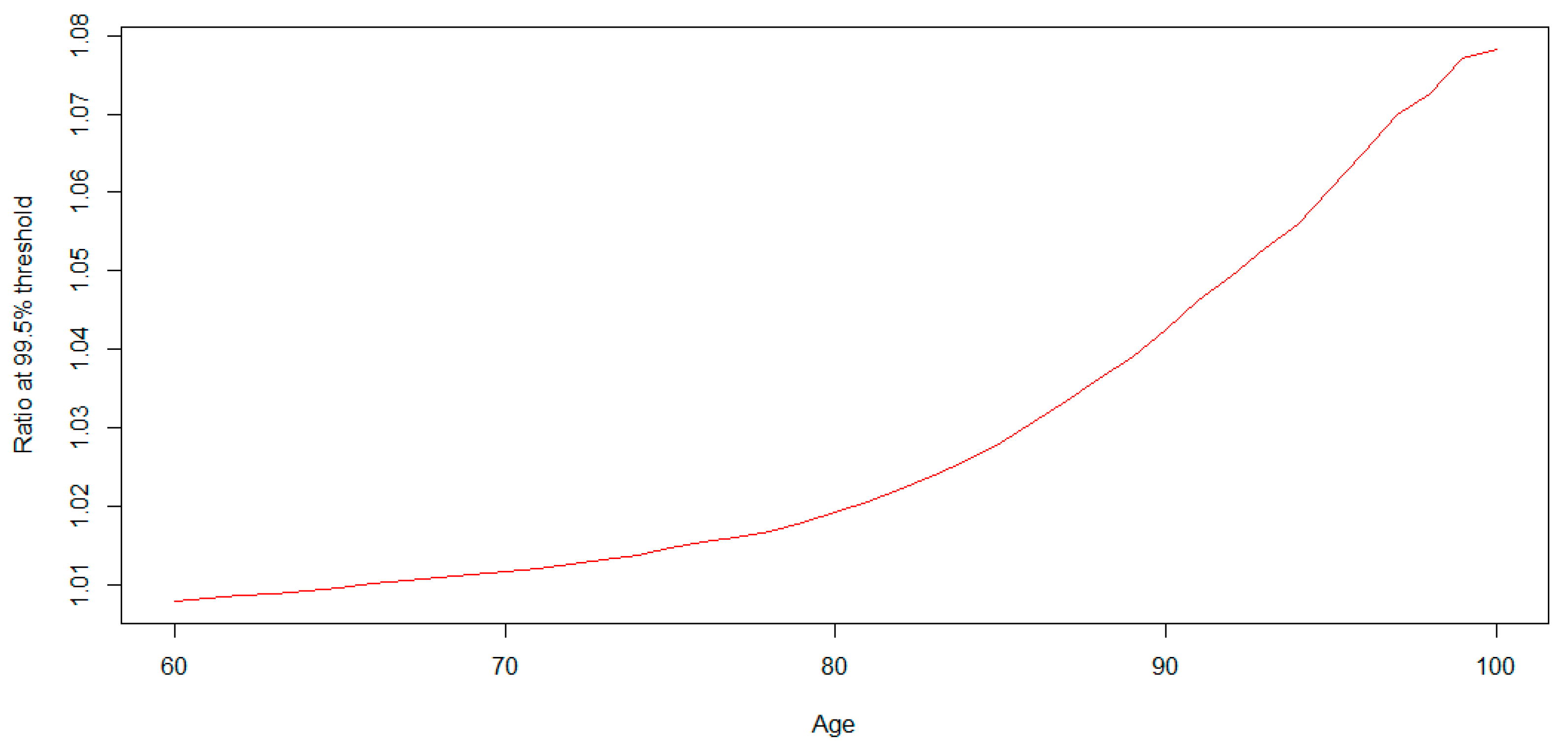
However, the random nature of the mortality distribution in a given year has consequences for the assessment of the capital required to protect against adverse deviations in mortality. In the specific context of a life annuity plan, following a logic analogous to that of the Solvency 2 standard, we are led to consider the 99.5% quantile of the distribution of residual life expectancies induced by frailty as a proxy for the SCR6. For each age from 60 to 100, we obtain the following results (Figure 13) for the ratio between this quantile and the expectation, from a direct Monte-Carlo approach:
Weighted by the age structure of the French population, the average ratio is around 101.3%.
For its part, the delegated regulation7 imposes a 20% discount on death rates when calculating the SCR associated with longevity risk (cf. art. 138 of delegated regulation EU n°2015/35), which leads to a capital requirement equal to 10% of the expectation.
This means that the volatility observed in annual death rates explains around 12% of the longevity SCR.
4. Conclusions and Discussion
The use of a Gamma frailty model enables us to correctly account for the annual variations in mortality levels observed throughout France.
Incorporating these variations into the fitting of a forward-looking log-Poisson model poses no major difficulty, and a two-stage parameter estimation process enables us to use conventional likelihood maximisation algorithms.
The results obtained show that the impact of this additional volatility is negligible on the central tendency indicators. However, those results follow the assumption that the shocks are mean-centred. This document provides a more general structure to perform prospective analyses under situations of durable deterioration or amelioration of mortality (i.e., consider ).
On the other hand, there is a material impact on the capital requirement associated with longevity risk, with just under 15% of this requirement being induced by the presence of this volatility. The remainder is associated with uncertainty about the trend in death rates.
Thus, while the main hazard associated with the construction of a prospective mortality table remains the uncertainty attached to the determination of the trend (see Juillard et al. (2008), Juillard and Planchet (2006) and Plat (2009) for detailed analyses on this point), considering these short-term fluctuations in mortality levels provides a better understanding of the determinants of longevity risk.
Finally, an important limitation of the proposed model is that the annual shock is applied with the same intensity to all ages. The determinants of shocks of this type over the last 40 years (typically heatwaves and/or flu epidemics or COVID-19) mainly concern older age groups (over 65). The model should, therefore, be refined on this point. However, this limitation needs to be put into perspective, as applications of this model mainly concern pension schemes, where participants are older.
Author Contributions
Conceptualization, F.P.; Methodology, G.G.d.L.P.; Software, G.G.d.L.P.; Data curation, G.G.d.L.P.; Writing—original draft, F.P.; supervision—F.P. All authors have read and agreed to the published version of the manuscript.
Funding
This research received no external funding.
Data Availability Statement
The data presented in this study are available on request from the corresponding author.
Conflicts of Interest
Authors Frédéric Planchet and Guillaume Gautier de la Plaine were employed by the company Prim’Act. The authors declare that the research was conducted in the absence of any commercial or financial relationships that could be construed as a potential conflict of interest. The company Prim’Act had no role in the design of the study; in the collection, analyses, or interpretation of data; in the writing of the manuscript, or in the decision to publish the results.
Appendix A

Table A1.
Calibrated model coefficients (1/3).
| Alpha | ||||||||
|---|---|---|---|---|---|---|---|---|
| Age | Model Studied | LC Reference Model | Age | Model Studied | LC Reference Model | Age | Model Studied | LC Reference Model |
| 0 | −5.6542 | −5.6553 | 36 | −7.0173 | −7.0186 | 72 | −4.0422 | −4.0456 |
| 1 | −7.3447 | −7.3457 | 37 | −6.9390 | −6.9396 | 73 | −3.9592 | −3.9625 |
| 2 | −8.2790 | −8.2804 | 38 | −6.8474 | −6.8480 | 74 | −3.8668 | −3.8713 |
| 3 | −8.6679 | −8.6695 | 39 | −6.7630 | −6.7633 | 75 | −3.7867 | −3.7882 |
| 4 | −8.9672 | −8.9721 | 40 | −6.6729 | −6.6733 | 76 | −3.6851 | −3.6862 |
| 5 | −9.0765 | −9.0803 | 41 | −6.5862 | −6.5867 | 77 | −3.5790 | −3.5803 |
| 6 | −9.1958 | −9.2028 | 42 | −6.4878 | −6.4880 | 78 | −3.4774 | −3.4791 |
| 7 | −9.2892 | −9.2924 | 43 | −6.3872 | −6.3877 | 79 | −3.3674 | −3.3679 |
| 8 | −9.4087 | −9.4124 | 44 | −6.2849 | −6.2854 | 80 | −3.2163 | −3.2216 |
| 9 | −9.3935 | −9.4009 | 45 | −6.1800 | −6.1803 | 81 | −3.0838 | −3.0881 |
| 10 | −9.4223 | −9.4329 | 46 | −6.0917 | −6.0922 | 82 | −2.9510 | −2.9556 |
| 11 | −9.3577 | −9.3662 | 47 | −5.9813 | −5.9817 | 83 | −2.8178 | −2.8236 |
| 12 | −9.2768 | −9.2809 | 48 | −5.8840 | −5.8845 | 84 | −2.6937 | −2.7014 |
| 13 | −9.1674 | −9.1742 | 49 | −5.7947 | −5.7952 | 85 | −2.5725 | −2.5850 |
| 14 | −8.9411 | −8.9443 | 50 | −5.7068 | −5.7077 | 86 | −2.4381 | −2.4498 |
| 15 | −8.6907 | −8.6949 | 51 | −5.6157 | −5.6166 | 87 | −2.3015 | −2.3126 |
| 16 | −8.4690 | −8.4721 | 52 | −5.5399 | −5.5411 | 88 | −2.1619 | −2.1733 |
| 17 | −8.2022 | −8.2047 | 53 | −5.4596 | −5.4605 | 89 | −2.0266 | −2.0390 |
| 18 | −7.9805 | −7.9814 | 54 | −5.3712 | −5.3722 | 90 | −1.8871 | −1.9001 |
| 19 | −7.7424 | −7.7441 | 55 | −5.2853 | −5.2866 | 91 | −1.7522 | −1.7651 |
| 20 | −7.6642 | −7.6654 | 56 | −5.2062 | −5.2078 | 92 | −1.6216 | −1.6351 |
| 21 | −7.6042 | −7.6051 | 57 | −5.1270 | −5.1289 | 93 | −1.4936 | −1.5072 |
| 22 | −7.5935 | −7.5952 | 58 | −5.0598 | −5.0611 | 94 | −1.3657 | −1.3777 |
| 23 | −7.5824 | −7.5837 | 59 | −4.9902 | −4.9925 | 95 | −1.2453 | −1.2594 |
| 24 | −7.5520 | −7.5540 | 60 | −4.9156 | −4.9178 | 96 | −1.1239 | −1.1367 |
| 25 | −7.5513 | −7.5531 | 61 | −4.8551 | −4.8570 | 97 | −1.0154 | −1.0262 |
| 26 | −7.5195 | −7.5211 | 62 | −4.7853 | −4.7877 | 98 | −0.9056 | −0.9177 |
| 27 | −7.4982 | −7.4995 | 63 | −4.7165 | −4.7182 | 99 | −0.8059 | −0.8166 |
| 28 | −7.4795 | −7.4816 | 64 | −4.6552 | −4.6571 | 100 | −0.7093 | −0.7208 |
| 29 | −7.4393 | −7.4409 | 65 | −4.5875 | −4.5894 | 101 | −0.6286 | −0.6345 |
| 30 | −7.3880 | −7.3899 | 66 | −4.5141 | −4.5163 | 102 | −0.5389 | −0.5481 |
| 31 | −7.3594 | −7.3607 | 67 | −4.4558 | −4.4580 | 103 | −0.4581 | −0.4679 |
| 32 | −7.3008 | −7.3012 | 68 | −4.3774 | −4.3802 | 104 | −0.4095 | −0.4185 |
| 33 | −7.2536 | −7.2544 | 69 | −4.2982 | −4.3005 | 105 | −0.4625 | −0.4652 |
| 34 | −7.1764 | −7.1771 | 70 | −4.2170 | −4.2209 | |||
| 35 | −7.1106 | −7.1110 | 71 | −4.1381 | −4.1415 | |||
Table A2.
Calibrated model coefficients (2/3).
| Beta | ||||||||
|---|---|---|---|---|---|---|---|---|
| Age | Model Studied | LC Reference Model | Age | Model Studied | LC Reference Model | Age | Model Studied | LC Reference Model |
| 0 | 0.0033 | 0.0033 | 36 | 0.0120 | 0.0120 | 72 | 0.0070 | 0.0071 |
| 1 | 0.0115 | 0.0115 | 37 | 0.0115 | 0.0115 | 73 | 0.0070 | 0.0071 |
| 2 | 0.0114 | 0.0114 | 38 | 0.0123 | 0.0123 | 74 | 0.0075 | 0.0077 |
| 3 | 0.0118 | 0.0117 | 39 | 0.0119 | 0.0118 | 75 | 0.0090 | 0.0091 |
| 4 | 0.0130 | 0.0131 | 40 | 0.0129 | 0.0129 | 76 | 0.0094 | 0.0094 |
| 5 | 0.0121 | 0.0118 | 41 | 0.0134 | 0.0135 | 77 | 0.0097 | 0.0097 |
| 6 | 0.0097 | 0.0102 | 42 | 0.0140 | 0.0140 | 78 | 0.0096 | 0.0097 |
| 7 | 0.0145 | 0.0146 | 43 | 0.0137 | 0.0137 | 79 | 0.0099 | 0.0098 |
| 8 | 0.0119 | 0.0121 | 44 | 0.0135 | 0.0136 | 80 | 0.0136 | 0.0129 |
| 9 | 0.0126 | 0.0127 | 45 | 0.0132 | 0.0133 | 81 | 0.0139 | 0.0134 |
| 10 | 0.0144 | 0.0138 | 46 | 0.0136 | 0.0137 | 82 | 0.0141 | 0.0137 |
| 11 | 0.0114 | 0.0118 | 47 | 0.0128 | 0.0127 | 83 | 0.0142 | 0.0137 |
| 12 | 0.0165 | 0.0162 | 48 | 0.0122 | 0.0122 | 84 | 0.0115 | 0.0107 |
| 13 | 0.0143 | 0.0142 | 49 | 0.0108 | 0.0108 | 85 | 0.0083 | 0.0073 |
| 14 | 0.0151 | 0.0151 | 50 | 0.0106 | 0.0106 | 86 | 0.0065 | 0.0057 |
| 15 | 0.0155 | 0.0151 | 51 | 0.0099 | 0.0099 | 87 | 0.0059 | 0.0054 |
| 16 | 0.0180 | 0.0182 | 52 | 0.0093 | 0.0093 | 88 | 0.0056 | 0.0052 |
| 17 | 0.0171 | 0.0171 | 53 | 0.0093 | 0.0093 | 89 | 0.0057 | 0.0054 |
| 18 | 0.0185 | 0.0187 | 54 | 0.0095 | 0.0094 | 90 | 0.0051 | 0.0049 |
| 19 | 0.0183 | 0.0180 | 55 | 0.0093 | 0.0092 | 91 | 0.0049 | 0.0048 |
| 20 | 0.0170 | 0.0169 | 56 | 0.0082 | 0.0080 | 92 | 0.0044 | 0.0046 |
| 21 | 0.0158 | 0.0158 | 57 | 0.0082 | 0.0081 | 93 | 0.0039 | 0.0041 |
| 22 | 0.0146 | 0.0146 | 58 | 0.0067 | 0.0066 | 94 | 0.0026 | 0.0030 |
| 23 | 0.0156 | 0.0156 | 59 | 0.0061 | 0.0059 | 95 | 0.0023 | 0.0027 |
| 24 | 0.0132 | 0.0134 | 60 | 0.0050 | 0.0049 | 96 | 0.0016 | 0.0024 |
| 25 | 0.0126 | 0.0127 | 61 | 0.0042 | 0.0041 | 97 | 0.0008 | 0.0014 |
| 26 | 0.0113 | 0.0115 | 62 | 0.0039 | 0.0038 | 98 | −0.0005 | 0.0004 |
| 27 | 0.0111 | 0.0112 | 63 | 0.0040 | 0.0039 | 99 | −0.0013 | −0.0006 |
| 28 | 0.0107 | 0.0108 | 64 | 0.0042 | 0.0042 | 100 | −0.0002 | −0.0001 |
| 29 | 0.0088 | 0.0088 | 65 | 0.0038 | 0.0038 | 101 | 0.0018 | 0.0022 |
| 30 | 0.0103 | 0.0102 | 66 | 0.0046 | 0.0046 | 102 | 0.0044 | 0.0047 |
| 31 | 0.0111 | 0.0110 | 67 | 0.0050 | 0.0051 | 103 | 0.0046 | 0.0048 |
| 32 | 0.0107 | 0.0106 | 68 | 0.0047 | 0.0047 | 104 | 0.0046 | 0.0053 |
| 33 | 0.0105 | 0.0104 | 69 | 0.0059 | 0.0059 | 105 | 0.0046 | 0.0051 |
| 34 | 0.0106 | 0.0105 | 70 | 0.0055 | 0.0055 | |||
| 35 | 0.0114 | 0.0113 | 71 | 0.0063 | 0.0064 | |||
Table A3.
Calibrated model coefficients (3/3).
| Kappa | |||||
|---|---|---|---|---|---|
| Age | Model Studied | LC Reference Model | Age | Model Studied | LC Reference Model |
| 2000 | 24.4565 | 24.4761 | 2030 | −43.8008 | −43.8043 |
| 2001 | 24.4627 | 24.5265 | 2031 | −45.9908 | −45.9945 |
| 2002 | 21.2073 | 21.2070 | 2032 | −48.1809 | −48.1847 |
| 2003 | 18.4710 | 18.4083 | 2033 | −50.3709 | −50.3750 |
| 2004 | 10.9651 | 10.9513 | 2034 | −52.5610 | −52.5652 |
| 2005 | 9.4399 | 9.4231 | 2035 | −54.7510 | −54.7554 |
| 2006 | 6.0386 | 6.0366 | 2036 | −56.9410 | −56.9456 |
| 2007 | 3.1599 | 3.1578 | 2037 | −59.1311 | −59.1358 |
| 2008 | 1.4649 | 1.4631 | 2038 | −61.3211 | −61.3260 |
| 2009 | 1.6981 | 1.6984 | 2039 | −63.5112 | −63.5163 |
| 2010 | −1.1863 | −1.1865 | 2040 | −65.7012 | −65.7065 |
| 2011 | −4.7123 | −4.7140 | 2041 | −67.8912 | −67.8967 |
| 2012 | −6.6593 | −6.6691 | 2042 | −70.0813 | −70.0869 |
| 2013 | −8.5651 | −8.5639 | 2043 | −72.2713 | −72.2771 |
| 2014 | −12.6304 | −12.6243 | 2044 | −74.4614 | −74.4673 |
| 2015 | −9.8526 | −9.8338 | 2045 | −76.6514 | −76.6575 |
| 2016 | −13.5803 | −13.5743 | 2046 | −78.8414 | −78.8478 |
| 2017 | −15.8335 | −15.8386 | 2047 | −81.0315 | −81.0380 |
| 2018 | −15.6887 | −15.6650 | 2048 | −83.2215 | −83.2282 |
| 2019 | −16.4993 | −16.4493 | 2049 | −85.4116 | −85.4184 |
| 2020 | −16.1564 | −16.2296 | 2050 | −87.6016 | −87.6086 |
| 2021 | −24.0904 | −24.0924 | 2051 | −89.7916 | −89.7988 |
| 2022 | −26.2805 | −26.2826 | 2052 | −91.9817 | −91.9891 |
| 2023 | −28.4705 | −28.4728 | 2053 | −94.1717 | −94.1793 |
| 2024 | −30.6606 | −30.6630 | 2054 | −96.3618 | −96.3695 |
| 2025 | −32.8506 | −32.8532 | 2055 | −98.5518 | −98.5597 |
| 2026 | −35.0406 | −35.0435 | 2056 | −100.7418 | −100.7499 |
| 2027 | −37.2307 | −37.2337 | 2057 | −102.9319 | −102.9401 |
| 2028 | −39.4207 | −39.4239 | 2058 | −105.1219 | −105.1304 |
| 2029 | −41.6108 | −41.6141 | 2059 | −107.3120 | −107.3206 |
| 2060 | −109.5020 | −109.5108 | |||
| 1 | It should be remembered that Lee and Carter’s initial model is not a probabilistic model, and simply proposes a parsimonious decomposition of interactions between age and year in the structure of mortality rates across a country. |
| 2 | https://cran.r-project.org/web/packages/Rsolnp/index.html (accessed on 31 December 2023). |
| 3 | https://cran.r-project.org/web/packages/demography/index.html (accessed on 31 December 2023). |
| 4 | https://www.ressources-actuarielles.net/C1256F13006585B2/0/39B54166464089AFC12572B0003D88C2/$FILE/20230921_FP.pdf?OpenElement (accessed on 31 December 2023). |
| 5 | https://actudactuaires.typepad.com/laboratoire/2021/03/mortalit%C3%A9-en-france-en-2020-suite.html (accessed on 31 December 2023). |
| 6 | The SCR is the minimum capital required to control the probability of ruin at one year in the sense of the economic balance sheet at the level of 0.5%. |
| 7 | EU Delegated Regulation n°2015/35: https://eur-lex.europa.eu/legal-content/FR/TXT/?uri=CELEX:32015R0035 (accessed on 31 December 2023). |
References
- Agalva, Élisabeth, and Nathalie Blanpain. 2021. Projections de Population 2021–2070. Insee Résultats. Paris: INSEE. [Google Scholar]
- Barbi, Elisabetta. 1999. Eterogeneità Della Popolazione e Sopravvivenza Umana: Prospettive Metodologiche ed Applicazioni alle Generazioni Italiane 1870–1895. Ph.D. thesis, Dipartimento Statistico, Università degli Studi di Firenze, Florence, Italy; 91p. [Google Scholar]
- Barbi, Elisabetta, Graciella Casellic, and Jacques Vallin. 2003. Hétérogénéité des générations et âge extrême de la vie. Population 58: 45–68. [Google Scholar] [CrossRef]
- Bongaarts, John. 2004. Long-range trends in adults mortality: Models and projection methods. Demography 42: 23–49. [Google Scholar] [CrossRef] [PubMed]
- Brouhns, Natacha, Michael Denuit, and Jeroen K. Vermunt. 2002. A Poisson log-bilinear regression approach to the construction of projected lifetables. Insurance, Mathematic and Economics 31: 373–93. [Google Scholar] [CrossRef]
- Carannante, Maria, Valeria D’Amato, Steven Haberma, and Massimilliano Menzietti. 2023. Frailty-based Lee–Carter family of stochastic mortality models. Quality and Quantity. [Google Scholar] [CrossRef]
- Currie, Ian, Maria Durban, and Paul Eilers. 2003. Using P-splines to extrapolate two-dimensional Poisson data. Paper presented at the 18th International Workshop on Statistical Modelling, Leuven, Belgium, July 7–11. [Google Scholar]
- Debonneuil, Edouard. 2015. Parametric age-dependent mortality model, for applications to retirement portfolios. In Actuarial Thesis. Lyon: ISFA. [Google Scholar]
- Ghalanos, Alexios, and Stefan Theussl. 2015. Rsolnp: General Non-Linear Optimization. Available online: https://cran.r-project.org/package=Rsolnp (accessed on 31 December 2023).
- Guette, Vivien. 2010. La prise en compte des catastrophes dans la modélisation de la mortalité. In Actuary Thesis. Lyon: ISFA. [Google Scholar]
- Guilbaud, Corentin. 2018. Nouveaux modèles d’analyse et de projection de la mortalité, application a la population française. In Mémoire d’Actuaire. Paris: Dauphine. [Google Scholar]
- Hyndman, Rob. 2023. Demography: Forecasting Mortality, Fertility, Migration and Population Data. Available online: https://cran.r-project.org/package=demography/index.html (accessed on 31 December 2023).
- Juillard, Marc, and Frederic Planchet. 2006. Mesure de l’incertitude tendancielle sur la mortalité—Application à un régime de rentes. Assurances et Gestion des Risques 75: 357–74. [Google Scholar]
- Juillard, Marc, Frédéric Planchet, and Pierre E. Thérond. 2008. Perturbations extrêmes sur la dérive de mortalité anticipée. Assurances et Gestion des Risques 76: 1–11. [Google Scholar]
- Lee, Ronald D., and Lawrence R. Carter. 1992. Modeling and forecasting us mortality. Journal of the American Statistical Association 87: 659–71. [Google Scholar]
- Planchet, Frédéric, and Pierre E. Thérond. 2011. Modélisation Statistique des Phénomènes de Durée—Applications Actuarielles. Paris: Economica. [Google Scholar]
- Plat, Richard. 2009. On stochastic mortality modelling. Insurance: Mathematics and Economics 45: 393–404. [Google Scholar]
- Robben, Jens, and Katrien Antonio. 2023. Catastrophe risk in a stochastic multi-population mortality model. arXiv arXiv:2306.15271. [Google Scholar]
- Thatcher, A. R. 1999. The Long-term Pattern of Adult Mortality and the Highest Attained Age. Journal of the Royal Statistical Society 162: 5–43. [Google Scholar] [CrossRef] [PubMed]
- Vaupel, James W., Kenneth Manton, and Eric Stallard. 1979. The impact of heterogeneity in individual frailty on the dynamics of mortality. Demography 16: 439–54. [Google Scholar] [CrossRef] [PubMed]
- Ye, Yinyu. 1987. Interior Algorithms for Linear, Quadratic, and Linearly Constrained Non-Linear Programming. Ph.D. thesis, Department of EES Stanford University, Stanford, CA, USA. [Google Scholar]
Figure 1.
Annual variation in global mortality rate in France (1982 to 2022).

Figure 2.
Comparison of the coefficients to those of a Lee–Carter model.

Figure 3.
Mortality forces by age.

Figure 4.
Mortality rates by age from 90 to 105 years.

Figure 5.
Mortality rates by year for selected ages.

Figure 6.
Mortality force ratio over the entire age range and prospective analysis period (2021 to 2060).
Figure 6.
Mortality force ratio over the entire age range and prospective analysis period (2021 to 2060).

Figure 7.
Average mortality rate per year, all ages combined, from 2021 to 2060.

Figure 8.
Trends in prospective residual life expectancy by age.

Figure 9.
Change in prospective residual life expectancy from age 90 to 105.

Figure 10.
Prospective residual life expectancy by year.

Figure 11.
Trend in prospective residual life expectancy by year at age 96.

Figure 12.
Evolution of prospective residual life expectancies from age 65 to 105 for selected years, with a new volatility coefficient.
Figure 12.
Evolution of prospective residual life expectancies from age 65 to 105 for selected years, with a new volatility coefficient.

Figure 13.
Ratio between 99.5% quantile and expectation (SCR).

Table 1.
Results of the extension of the time coefficients k.
| m | p | |
|---|---|---|
| Model studied | −2.19 | 4401.98 |
| Lee–Carter reference model | −2.19 | 4402.33 |
Disclaimer/Publisher’s Note: The statements, opinions and data contained in all publications are solely those of the individual author(s) and contributor(s) and not of MDPI and/or the editor(s). MDPI and/or the editor(s) disclaim responsibility for any injury to people or property resulting from any ideas, methods, instructions or products referred to in the content. |
© 2024 by the authors. Licensee MDPI, Basel, Switzerland. This article is an open access article distributed under the terms and conditions of the Creative Commons Attribution (CC BY) license (https://creativecommons.org/licenses/by/4.0/).
Share and Cite
MDPI and ACS Style
Planchet, F.; Gautier de La Plaine, G. Adding Shocks to a Prospective Mortality Model. Risks 2024, 12, 57. https://doi.org/10.3390/risks12030057
AMA Style
Planchet F, Gautier de La Plaine G. Adding Shocks to a Prospective Mortality Model. Risks. 2024; 12(3):57. https://doi.org/10.3390/risks12030057
Chicago/Turabian StylePlanchet, Frédéric, and Guillaume Gautier de La Plaine. 2024. "Adding Shocks to a Prospective Mortality Model" Risks 12, no. 3: 57. https://doi.org/10.3390/risks12030057
Note that from the first issue of 2016, this journal uses article numbers instead of page numbers. See further details here.