Article

Two-Population Mortality Forecasting: An Approach Based on Model Averaging

1
Bayes Business School, City, University of London, London EC1Y 8TZ, UK
2
DEAMS, University of Trieste, 34127 Trieste, Italy
*
Author to whom correspondence should be addressed.
Risks 2024, 12(4), 60; https://doi.org/10.3390/risks12040060
Submission received: 13 February 2024 / Revised: 15 March 2024 / Accepted: 21 March 2024 / Published: 27 March 2024

Abstract

:
The analysis of residual life expectancy evolution at retirement age holds great importance for life insurers and pension schemes. Over the last 30 years, numerous models for forecasting mortality have been introduced, and those that allow us to predict the mortality of two or more related populations simultaneously are particularly important. Indeed, these models, in addition to improving the forecasting accuracy overall, enable evaluation of the basis risk in index-based longevity risk transfer deals. This paper implements and compares several model-averaging approaches in a two-population context. These approaches generate predictions for life expectancy and the Gini index by averaging the forecasts obtained using a set of two-population models. In order to evaluate the eventual gain of model-averaging approaches for mortality forecasting, we quantitatively compare their performance to that of the individual two-population models using a large sample of different countries and periods. The results show that, overall, model-averaging approaches are superior both in terms of mean absolute forecasting error and interval forecast accuracy.

1. Introduction

In recent decades, as a consequence of life expectancy improvements and social and behavioural changes that have taken place in various countries, pension funds, annuities, and other insurance products that provide retirement income have become increasingly important. However, since these products are subjected to longevity risk, which refers to the systematic trend of mortality rates decreasing over time, it has become necessary to find effective models for forecasting mortality rates. Notably, several models have been developed to address this issue, including the Lee-Carter model (Lee and Carter 1992), its extension the Renshaw-Haberman model (Renshaw and Haberman 2006), the Cairns-Blake-Dowd model (Cairns et al. 2006) and its extensions—the M6, M7, and M8 models (Cairns et al. 2009)—and the Plat model (Plat 2009). In all these models, the mortality rates depend on two types of quantities: fixed parameters that represent the effect of age on the mortality and stochastic factors that represent the effect of cohort year and calendar year. All these quantities must be estimated using statistical techniques based on past data. Finally, the mortality rates are forecasted, extrapolating the stochastic factors on the more recent period. Originally, these models had been designed to forecast the mortality rates of single populations. Later, they were implemented in a multi-population framework by Li and Lee (2005). This class of models has become increasingly popular because it allows researchers to work simultaneously with different populations that are to some extent related (e.g., males and females in the same country or region), obtaining coherent forecasts; see Dowd et al. (2011), Li (2013), Yang et al. (2016), Enchev et al. (2017), and Shang et al. (2022). This means that these models are able to respect limitations and constraints that we set such as the biological ones like the sex gap between the life expectancy of females and males. As an instance of practical application, we can refer to the longevity risk transfer products where it is necessary to quantify the basis risk that is the systematic difference between the population mortality and the pension fund mortality; see Villegas et al. (2017).
As researchers continue to make progress in developing single-population and multi-population mortality forecasting models, there has also been a growing interest in model-averaging approaches in recent years; see Shang et al. (2011), Shang (2012), and Benchimol et al. (2016). The idea behind them is that forecasts are obtained by averaging models’ predictions using various weighting schemes. By adopting a model-averaging approach, we can avoid some potential drawbacks of using single or multi-population mortality forecasting models; see Hinne et al. (2020) and Benchimol et al. (2016). These models are affected by a sort of over-confidence in that they assume the selected model is the only one correct and will produce precise forecasts in any situation. This implies an all-or-nothing mentality. They could lead to large-scale forecasting errors (outliers) and incoherence: in the presence of new data (mortality rates of a different country, for instance), the selected model may no longer be optimal among those studied. Indeed, the model accuracy, on which optimal model selection depends, is heavily influenced by the dataset used in the selection process.
This paper aims at introducing and comparing model-averaging approaches in a two-population mortality forecasting context and quantitatively evaluating them, highlighting their differences and comparing them to specific two-population models. We used truncated life expectancy and the Gini index as metrics to capture the location and dispersion of the residual lifetime distribution. Our main conclusions are that a simple, equally weighted approach performs just as well as more sophisticated averaging approaches, and model-averaging approaches are overall superior in terms of mean absolute forecasting error and interval forecast accuracy to most common two-population models by considering a range of combinations of test and training periods and countries.
The remainder of this paper is organised as follows. In Section 2, we revisit some existing stochastic multi-population models in the literature with a particular focus on the two-population case. In Section 3, model-averaging approaches applied to two-population mortality forecasting are introduced from a theoretical point of view. In Section 4, we list the datasets that we use in our practical examples. In Section 5, the procedure implemented to obtain the quantitative results is described step-by-step. In Section 6, the results are presented and discussed. Finally, in Section 7, we summarise the most important findings of the previous sections and provide a future outlook.

2. Two-Population Mortality Models

Let us consider two populations, denoted by p = m , f , that represent males and females of one specific country, and assume that for both of them, the force of mortality is constant over each calendar year and age, so that the force of mortality coincides with the central death rate m x , t ( p ) . The number of deaths D x , t ( p ) in population p, year t, and age x, conditionally on the central death rate m x , t ( p ) , is assumed to follow a Poisson distribution:
D x , t ( p ) P o ( N x , t ( p ) m x , t ( p ) ) ,
where N x , t ( p ) is the central exposure to risk. In order to forecast central death rates, several models have been proposed in the last three decades following the original idea of Lee and Carter (1992). In all these models, the natural logarithm of mortality rates m x , t ( p ) , or of probability of death q x , t ( p ) ,1 is expressed as a function of two different types of quantities: time-dependent stochastic factors and age-dependent parameters. A relevant selection of these models is considered in this paper in their two-population form and summarised in Table 1.2 More precisely, in any given population, the mortality rates of both females ( m x , t f ) and males ( m x , t m ) are specified by one of the equations in 1–9 in Table 1. These models can be broadly classified as follows: models where the age is treated as categorical (1, 2, 8, and 9), as a quantitative variable (3–6) or hybrid (7); models which consider a cohort effect (2, 4, and 7) or not; models with a stochastic time factor common to both females and males populations (8 and 9) or models where the dependence between sexes only stems from the correlation in stochastic time factors; and models with one (1, 2, and 8), two (3, 4, 6, 7, and 9) or three stochastic time factors (5).

2.1. Model Estimation

The parameters of the models in Table 1 are usually estimated by maximizing the joint Poisson log-likelihood:
= p x t d x , t ( p ) ln ( N x , t ( p ) m x , t ( p ) ) N x , t ( p ) m x , t ( p ) ln ( d x , t ( p ) ! )
where d x , t ( p ) are the observed deaths in population p, year t, and age x. The mortality rates m x , t ( p ) for each model can be obtained from the corresponding equations in Table 1. The optimisation is performed using numerical algorithms. Note that for models 1–7, the log-likelihood for each population can be maximised separately.

2.2. Stochastic Factor Assumptions

From Table 1, it can be seen that the models considered depend on a number of stochastic factors. More precisely, each model contains a combination of (one or more of) the following terms: population-specific time indices κ t ( i , p ) , common time index κ t , and population-specific cohort effects γ t ( p ) . Inspired by Li et al. (2015), for the time indices κ t ( i , p ) (models 1–7, 9) we consider a combination of a random walk with drift and first-order autoregression AR(1). The rationale of this choice is that there is a stable relation between the period indices of males and females.
  • κ t ( i , m ) = μ ( i , m ) + κ t 1 ( i , m ) + Z t ( i , m ) , i = 1 , 2 , 3
  • κ t ( i , f ) = κ t ( i , m ) + ϕ ( i , f ) ( κ t 1 ( i , f ) κ t 1 ( i , m ) ) + Z t ( i , f ) , i = 1 , 2 , 3
where μ ( i , m ) are the drift parameters, ϕ ( i , f ) are the autoregressive parameters, and ( Z t ( i , p ) ) p = m , f are normal iid innovations.
For the time index κ t (models 8–9), we consider a random walk with drift:
  • κ t = μ + κ t 1 + Z t ,
where μ is the drift parameter, ϕ is the autoregressive parameter, and Z t are normal iid innovations.
Finally, for the cohort terms γ t x ( p ) (models 2, 4–7), we consider a combination of ARIMA(1, 1, 0) (see Villegas et al. (2017) and Dowd et al. (2010)) and first-order autoregression AR(1) (see Li et al. (2015)). Again, the rationale is that there is a stable relation between the cohort effects of males and females.
  • γ u ( m ) = ( 1 + ϕ ( m ) ) γ u 1 ( m ) ϕ ( m ) γ u 2 ( m ) + Y u ( m )
  • γ u ( f ) = γ u ( m ) + ϕ ( f ) ( γ u 1 ( f ) γ u 1 ( m ) ) + Y u ( f )
where ϕ ( m ) and ϕ ( f ) are the autoregressive parameters of the process, while ( Y u ( p ) ) p = m , f are normal iid innovations.
In models 1–7, the dependence between female and male mortality is derived from the autoregressive components. In model 8, the dependence is given by the shared time index κ t between female and male populations. In model 9, the dependence is derived by both the shared time index and the autoregressive component.

3. Model-Averaging Approaches

Suppose we have historical data on mortality for the period [ t 0 , t s ] , and we are interested in forecasting some mortality metric on the period [ t s + 1 , t n ] . The purpose of model-averaging approaches is to obtain forecasts of a given metric
U t ( p ) = f ( ( m x , t ( p ) ) x = 0 , , ω 1 )
that can be expressed as a function of mortality rates, where ω is the ultimate age, as an average of the forecasted metrics obtained using L different models. Notice that in this paper, we consider individual models listed in Table 1, and L = 9 . As an example of the metric U t ( p ) , we can use the j-years survival probability p x , t ( p ) j = exp { ( m x , t ( p ) + m x + 1 , t ( p ) + + m x + j 1 , t ( p ) ) } .
Let the metric of interest for the population p, in year t, and model l be
U ^ t ( p , l ) = f ( ( m ^ x , t ( p , l ) ) x = 0 , , ω 1 ) , l = 1 , , L
where m ^ x , t ( p , l ) is the forecasted mortality rate at age x, for the population p, in year t, obtained using model l. Following Fletcher (2018) and Shang (2012), the averaged metric is calculated as
U ^ t ( p , a v e r a g e ) = λ 1 U ^ t ( p , 1 ) + + λ L U ^ t ( p , L )
where λ L , , λ L are non-negative weights calculated based on the model-averaging approach considered dependently on the performance of the models in the validation period.
In this paper, we consider the following four model-averaging approaches:
  • Equal weights (EW):
    λ l E W = 1 L , l = 1 , , L .
    This method is the most simple, as all models are assigned the same weight; see Shang (2012). There is no penalisation or reward depending on the performance in the validation period.
  • Proportional weights (PW):
    λ l P R = 1 g l k = 1 L 1 g k , l = 1 , , L
    where g l = g ( U ^ t ( p , l ) , U t ( p , l ) ; p = m , f ; t = t s h + 1 , , t s ) is a strictly positive performance measure representing the performance of the model l in the validation period [ t s h + 1 , t s ] ; see Shang (2012). In this way, models that have poor performance in the validation period are penalised with smaller weights.
  • Weights based on the the softmax function (SM):
    λ l S M = exp { g l } k = 1 L exp { g k } , l = 1 , , L .
    The concept is similar to the proportional weights model-averaging approach, but here we penalise less the models with poor performance in the validation period and reward less the models with good performance. See also Benchimol et al. (2016) for a similar formulation.
  • Weights based on trimming (TR):
    λ l T R = 1 L ^ , if l is among the L ^ best models in the validation period , 0 , otherwise ,
    where the best models are determined in terms of the measure g l ; see Samuels and Sekkel (2017) and Shang (2012). With this method, we reward only the L ^ models that have the best performance in the validation period, assigning the same weight ( 1 L ^ ) for each one of them. In the following, we set L ^ equal to 3.
In the remainder of this paper, for the definition of measure g used to evaluate the models’ performance in the validation period, we adopt the mean absolute forecasting error (MAFE)
MAFE l = p = m , f t = t s h + 1 t s | U ^ t ( p , l ) U t ( p , l ) | P · h
where t s h + 1 and t s are the first and last years of the validation period. Notice that alternative measures could also have been considered. For example, one that also takes into account the number of parameters in the model.
Finally, regarding the metric in (4), we choose the residual life expectancy at age 55 truncated at age 90, which represents a location metric of mortality rates; see Dickson et al. (2019),
e ˚ 55 : 35 , t = j = 1 35 p 55 , t j 1 ( 1 1 2 q 55 + j 1 , t )
and the Gini index, calculated between 55 and 89, that represents the dispersion of mortality rates3
G 55 : 35 , t = 1 2 e ˚ 55 : 35 , t x = 55 89 y = 55 89 q 55 , t x 55 | 1   q 55 , t y 55 | 1   | x y | .
The Gini index is a metric that varies between the limits of 0 (perfect equality) and 1 (perfect inequality). For a length of life distribution, it is equal to zero if all individuals die at the same age and equal to one if all people die at age 0 and one individual dies at an infinitely old age. The choice of the Gini index as a metric representing the dispersion of mortality depends on the fact that, unlike other metrics such as interquartile range, variance, and standard deviation, it possesses all the desirable properties for an inequality index: population-size independence, mean or scale independence, and transfer principle; see Shkolnikov et al. (2003) for more details.

4. Data

In the following, we implement the multi-population models and the model-averaging approaches with historical mortality data from ten pairs of populations, namely the female and male populations of Australia, Canada, France, England and Wales, Italy, Japan, Netherlands, Spain, Sweden, and the US. The choice of these countries depends on the fact that they are developed with large populations, and their data are complete and easily obtainable in the Human Mortality Database (HMD). For these countries, we considered the age range between 55 and 89 for the mortality rates. The reason for this choice derives from the fact that most of the deaths are concentrated after the age of 55 years and that after the age of 90 years, we have fewer data, especially for the older cohorts, so this could lead to biased estimations of the models. Furthermore, we note that, at ages over 90, there is evidence of age misstatements that may lead to biased estimates of mortality indices. Moreover, this age range is the most relevant from an actuarial point of view; see Cairns et al. (2006). Finally, concerning the periods considered, we have two cases: in the first one, we have a 30-year rolling training period from 1950–1979 to 1975–2004 and a 15-year rolling test period from 1980–1994 to 2005–2019 (last year for which the data are available at the time of writing this paper); in the second one, we have a variable length training period from 1966–2004 to 1985–2004 and a 15-year fixed test period 2005–2019.

5. Implementation

Step-By-Step Procedure
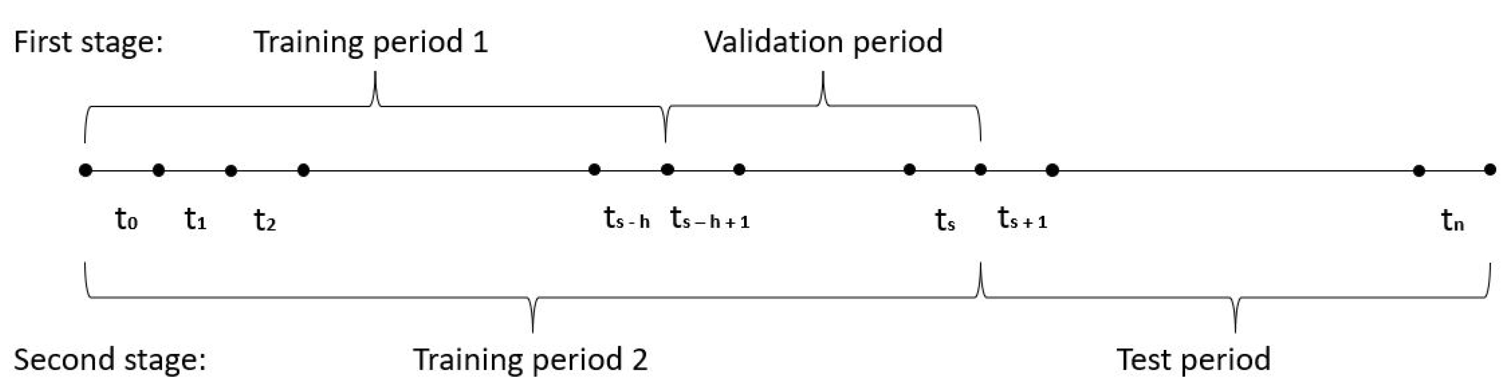
For a generic country, training period [ t 0 , t s ] , and test period [ t s + 1 , t n ] (see Figure 1), we follow the steps listed below:
  • First stage
    1.1
    We fit the two-population models (LC, RH, CBD, PLAT, M6, M7, M8, CF, and ACF) on the period [ t 0 , t s 10 ] (training period 1) using the StMoMo package; see Villegas et al. (2018). Notice that this implies h, i.e., the length of the validation period, is set equal to 10.
    1.2
    We simulate mortality rates for the period [ t s 9 , t s ] (validation period) using the models fitted in 1.1.
    1.3
    We calculate the corresponding truncated life expectancy and Gini index for each model as functions of the mortality rates obtained in 1.2 using Formulas (11) and (12).
    1.4
    We repeat steps 1.2 and 1.3 1000 times, and we obtain the forecasted truncated life expectancy and Gini index as the average of these for each model.
    1.5
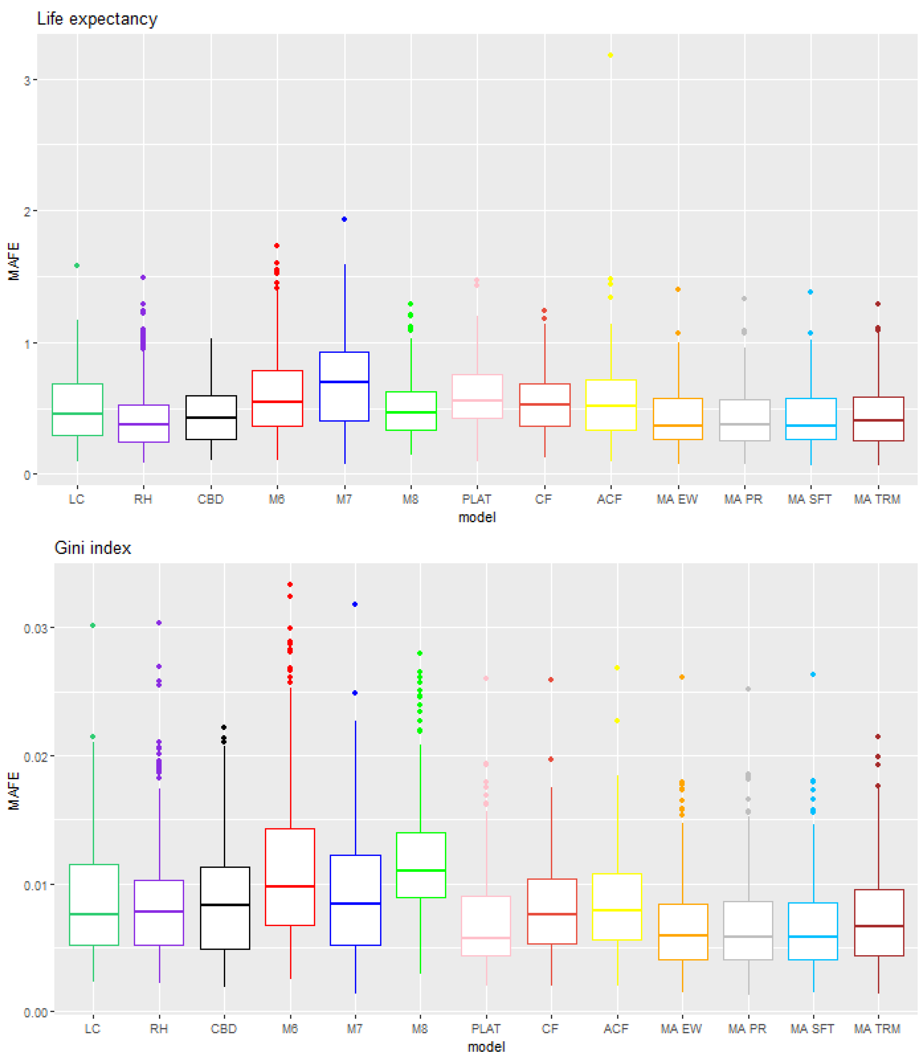
    We calculate the MAFE as the difference between forecasted truncated life expectancy and Gini index calculated in 1.4 and the historical ones (Formula (10)) for each model.
    1.6
    We calculate the weights of each model-averaging approach based on the MAFEs calculated in 1.5 using Formulas (6)–(9).
  • Second stage
    2.1
    We repeat step 1.1 using the period [ t 0 , t s ] (training period 2) instead of [ t 0 , t s 10 ] .
    2.2
    We repeat steps 1.2 and 1.3 using the period [ t s + 1 , t n ] (test period) instead of [ t s 9 , t s ] .
    2.3
    We repeat step 2.2 10,000 times4 and we obtain the forecasted truncated average life expectancy and Gini index as the average of these for each model.
    2.4
    For each model-averaging approach, we carry out 1 simulation from a multinomial distribution with parameters equal to 10,000, 9, and the vector of the weights obtained in 1.6. The result of this simulation will be a vector with 9 elements, which sum to 10,000, that represent the number of truncated life expectancy and Gini index trajectories that are considered in the model-averaging approach from the 9 two-population models.
    2.5
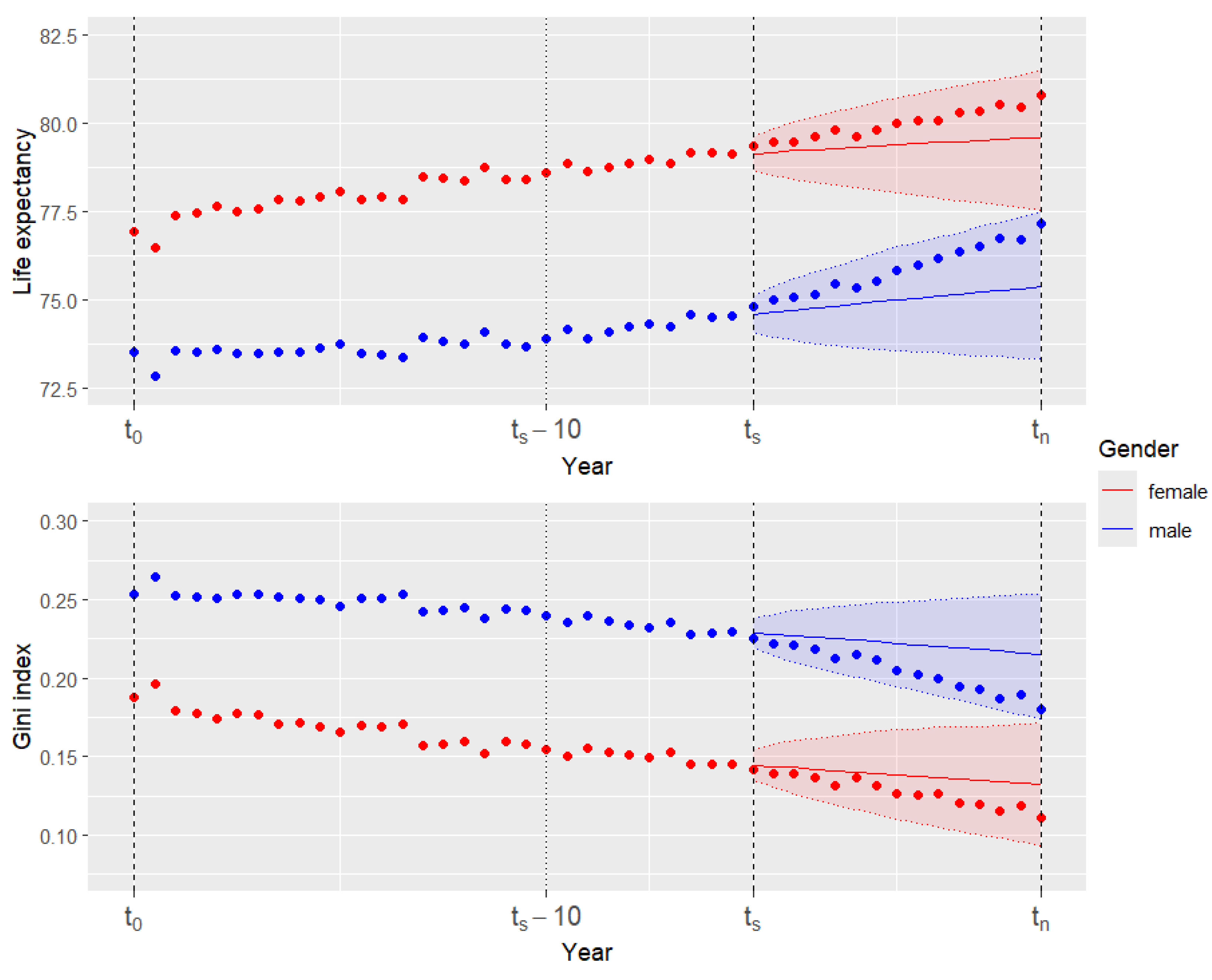
    Using the results of the simulation at point 2.4 as parameters, we resample by bootstrapping from the truncated life expectancy and Gini index trajectories obtained in step 2.3, and we average them using Formula (5) obtaining the forecasted truncated life expectancy and Gini index for all the model-averaging approaches. Similarly, we take the 5th and 95th percentile to build the 90% confidence forecasting intervals for the two metrics. See Figure 2 for an example of forecasted life expectancy and Gini index using the model-averaging approach with equal weights.
    2.6
    We calculate the MAFE as the difference between the forecasted truncated life expectancy and the Gini index calculated in 2.3 and 2.5 with the observed ones. Similarly, we compare the confidence forecasting intervals of the two metrics with the observed values in order to obtain the interval forecast accuracy that represents the proportion of times in which the observed truncated life expectancy and Gini index fall within the respective prediction intervals.

6. Results

Following Shang (2012), in order to evaluate the performance of each model, we must consider the goodness of both point and interval forecasts. For the first one, we consider the mean absolute forecasting error (MAFE; see Formula (10)), while for the second one, the interval forecast accuracy, here defined as the proportion of cases in which the observed life expectancy or Gini index falls within the 90% confidence forecasting interval, is considered. In Figure 3, we can find boxplots summarising the mean absolute forecasting errors for life expectancy and the Gini index obtained by all the models and model-averaging approaches previously mentioned in the rolling test period case. Figure 4 shows, for the rolling test period case, which is the best model, i.e., the one with the lowest MAFE, by period, country, and metric. Figure 5 and Figure 6 have the same content as Figure 3 and Figure 4 respectively, but for the fixed test period case. Finally, Table 2, Table 3, Table 4 and Table 5 and Table 6, Table 7, Table 8 and Table 9 report the interval forecast accuracy of the models by period, country, and metric, respectively, for rolling and fixed test period cases.

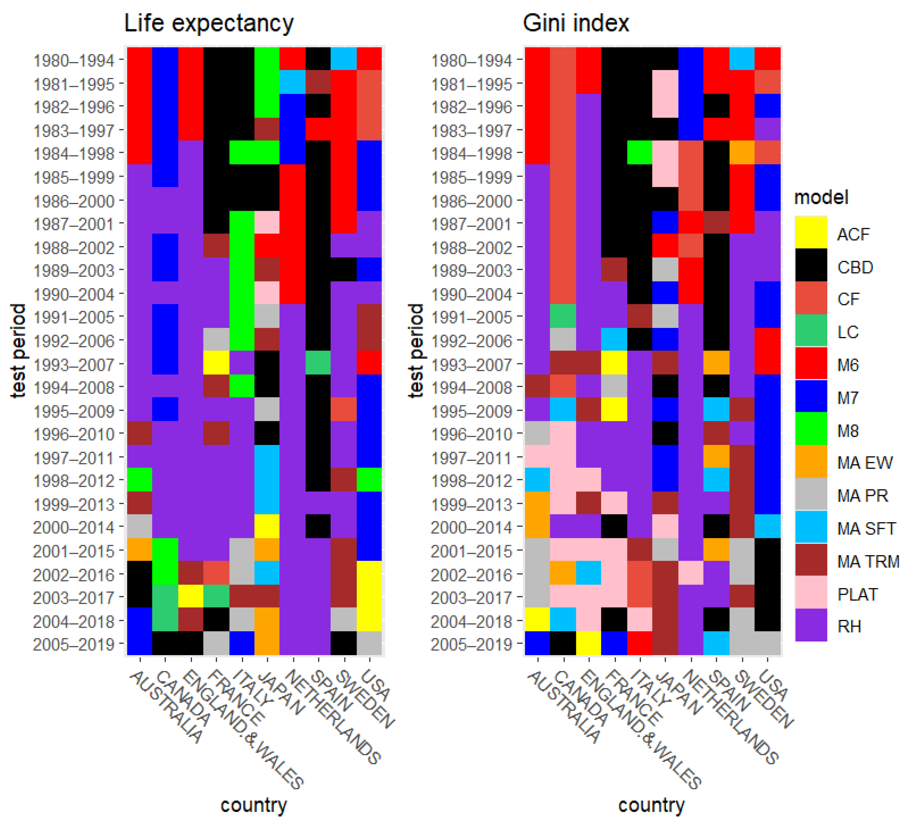
6.1. Rolling Test Period

Observing Figure 3, we can generally say that the best results, in terms of MAFE, are given by the model-averaging approaches based on equal and proportional weights and on the softmax function. They all present a median MAFE lower than 0.4 and 0.006, respectively, for life expectancy and the Gini index. The RH model is the third-best model (after model-averaging approaches with equal weights and with weights based on the softmax function) for life expectancy (but with weak performance for the Gini index), while the PLAT model is the best for the Gini index (but has weak performance for life expectancy). The model-averaging approach based on trimming has good overall performance as well. Indeed, it is overcome in terms of median MAFE only by the RH model for life expectancy and the PLAT model for the Gini index. Among the other models, good results are given by the CBD model regarding life expectancy and by the CF model for the Gini index. The worst results here are found in the M7 model for life expectancy and the M6 and M8 models for the Gini index. Other models, such as LC and ACF, do not show remarkable results.
Figure 4 shows the model with the lowest MAFE by country and period. The RH model has the highest number of best performances for both life expectancy and the Gini index (34% and 26%),5 followed by the CBD model (17% and 17%). It is interesting to notice how here the M7 model is the third-best model for life expectancy, despite it being the worst one in terms of median MAFE, and the M6 model is the third-best for the Gini index, despite being the second-worst one in terms of median MAFE. Focusing on the model-averaging approaches, it can be noted that they are seldom the best ones. Among them, the trimming averaging approach has the highest proportion of winning cases (7% and 8%). These results, even if they appear to contradict those in Figure 3, are easily explained. Indeed, model-averaging approaches have solid performance (ranking in the top five positions in terms of lowest MAFE) across all countries, periods, and metrics. On the contrary, individual models that are the best for specific combinations of countries and periods, such as M7 for life expectancy and M6 for the Gini index, are overall among the worst, as shown in Figure 3. Consequently, the advantage of model averaging is striking, in particular when several countries must be considered and models must be updated on different training periods.
Table 2, Table 3, Table 4 and Table 5 show the interval forecast accuracy results. As happened for the median MAFE analysis, the model-averaging approaches based on equal and proportional weights and on the softmax function are the best ones, with an interval forecast accuracy of 97% for the life expectancy and 98% for the Gini index. They are followed by the model-averaging approach based on trimming (93% and 94%). Among the other models, we have that the RH model has an interval forecast accuracy of 81% for the life expectancy (lower than the LC and CBD models), and the PLAT model has an interval forecast accuracy of 92% for the Gini index (the highest outside the model-averaging approaches, followed by M7 and LC models).
In the following, we report other findings from the tables and figures mentioned above, focusing particularly on the analysis by country, period, and metric considered. In Figure 4, we notice how the best model changes over time due to changes in mortality trends, such as the slowing down in mortality improvements observed in several developed countries since 2010; see Djeundje et al. (2022). Similar behaviour can also be noticed in Table 2 and Table 4 for the forecast interval accuracy. In this regard, the evolution of the RH model’s performance is enlightening. Indeed, it goes from being the best model for life expectancy in most periods considered to becoming the second-worst in the last test period (see Figure 5). This fact strengthens the motivation to choose a model-averaging approach that considers all or several models over a single model.
In Figure 4 and Table 3 and Table 5, we observe how most individual models have a good performance in terms of interval forecast accuracy and number of cases with the lowest MAFE, for at least one country. However, there are also countries where these models show poor performance, with low interval forecast accuracy and no cases in which they are the best. This is a consequence of the fact that each country has a specific mortality trend, which is fitted better by certain models than others. On the other hand, model-averaging approaches have more robust results with good performance in all the countries.
In conclusion, observing Table 2, Table 3, Table 4 and Table 5 and Figure 3 and Figure 4, we see how the performance of the models varies substantially based on whether we consider life expectancy or the Gini index, while for the model-averaging approaches there are no large-scale variations. This means that the latter are more robust even regarding the choice of the metric considered.

6.2. Fixed Test Period

Observing Figure 5, we see how, similarly to what happened with the rolling test period case, the model-averaging approaches based on equal and proportional weights and on the softmax function have the best results in terms of MAFE. They all present a median MAFE lower than 0.2 and 0.004 for life expectancy and the Gini index, respectively. Furthermore, notable performance in terms of median MAFE is obtained with the LC model for both the Gini index and life expectancy, while here the RH model is among the worst for life expectancy, and the Plat model is now overcome by other models regarding the Gini index. The model-averaging approach based on trimming has a higher MAFE, and it is outperformed by other models such as CBD and ACF for life expectancy and M7 and ACF for the Gini index. Indeed, the trimming based averaging approach heavily relies on the RH (for life expectancy) and PLAT (for Gini index) models, which have poor performance in the test period considered.
Figure 6 shows the model with the lowest MAFE by period and country. The RH model still has the highest number of best performances for life expectancy (16%),6 while the M7 model has the highest number for the Gini index (23%). All the model-averaging approaches here have good performance; indeed, they globally account for 40% for life expectancy and 37% for the Gini index, with the model-averaging approach with proportional weights showing the best results in both cases (12% and 17%). Other remarkable results are obtained with the CBD and M7 models for life expectancy, and the PLAT model regarding the Gini index. As in the rolling period case, the apparent discrepancy between between some results in Figure 5 and those in Figure 6 is explained by the superior robustness of the averaging approaches over the individual models.
Table 6, Table 7, Table 8 and Table 9 show the proportion of cases in which the observed metrics fall in the forecasting intervals. As was the case for the rolling test period case, the model-averaging approaches based on equal and proportional weights and on the softmax function have the highest interval forecast accuracy, with 98% for life expectancy and 99% for the Gini index. They are followed by the model-averaging approach based on trimming (94% and 93%). Among the other models, we find that the LC (90%) and ACF (87%) models show good results for life expectancy, while the M7 (91%) and LC (89%) models show good results for the Gini index. The RH model here is the worst model for life expectancy forecast accuracy as well as the Gini index (43% and 44%), while the PLAT model performance decreases for the Gini index (from 92% to 74%). This is an additional demonstration that it is not always optimal to rely on models that performed well previously.
To conclude, in Table 6, Table 7, Table 8 and Table 9 and Figure 5 and Figure 6, we notice that, compared with the rolling test period case, there is less variability in the models’ performance by training period as the test period remains fixed. A similar remark can be made with respect to the results by life expectancy and the Gini index. Instead, regarding the results by country, we observe how the performance variability remains, with many individual models performing well in some countries and badly in others. In contrast, the model-averaging approaches, except for the one based on trimming that is slightly weaker, show good results in all the countries considered.

7. Conclusions

In this paper, we compared the forecast performance of existing two-population models with those of four different model-averaging approaches. We considered ten countries and 46 different combinations of training and test periods, using truncated life expectancy and the Gini index as metrics. Our results show that model-averaging approaches outperformed the individual models, achieving superior results both in terms of MAFE (difference between the forecasted central truncated life expectancy and Gini index and the observed ones) and interval forecast accuracy (proportion of cases in which the observed values fall within the prediction interval). Among the model-averaging approaches, the best results are given by the ones with equal weights, proportional weights, and weights based on the the softmax function, while the one based on trimming shows a poorer performance, although it is still better than many individual models. The fact that the model-averaging approach based on trimming produces a higher MAFE on average is likely to be a consequence of changes in mortality trends: the models that perform well in the validation period do not necessarily perform equally well in the test period due to the speed up or slow down in the mortality improvements over the years. Finally, a further advantage of model-averaging approaches is that, while the performance of individual models is heavily affected by the choice of the metric (life expectancy or the Gini index), country, and period, the performance of the model-averaging approaches is shown to be more robust concerning this choice.
In terms of extensions of this research, a straightforward development could be considering multi-population models that simultaneously consider three or more populations rather than just two-population models. Furthermore, alternative measures of mean absolute forecasting error and interval forecast accuracy could be considered for comparing the goodness of forecasts of model-averaging approaches and traditional models.

Author Contributions

Conceptualization, P.M.; methodology, L.D.M., S.H. and P.M.; software, L.D.M. and P.M.; formal analysis, L.D.M.; investigation, L.D.M., S.H., P.M. and R.Z.; data curation, L.D.M.; writing—original draft preparation, L.D.M.; writing—review and editing, S.H., P.M. and R.Z.; supervision, S.H., P.M. and R.Z. All authors have read and agreed to the published version of the manuscript.

Funding

This research received no external funding

Data Availability Statement

The data presented in this study are available on request from the corresponding author.

Conflicts of Interest

The authors declare no conflicts of interest.

Notes

1
Probabilities of death q x can be calculated from the corresponding mortality rates m x by using the relation q x = m x / ( 1 + 1 2 m x ) , and vice versa, m x = q x / ( 1 1 2 q x ) .
2
For consistency, we use the Poisson distribution assumption coupled with the log-link function and mortality rates for models such as M6, M7, and M8, which usually are presented under a binomial assumption coupled with the logit-link function and probabilities of death.
3
The formula used here is an approximation for the Gini index at age 55, truncated at age 90, which includes an additional term accounting for the survival past age 90.
4
We carry out more simulations than in the first stage since here we consider the interval forecast accuracy in addition to the MAFE.
5
These percentages have been calculated as the ratio of the number of cases in which each model is the best over the total number of cases considered (260).
6
These percentages have been calculated as the ratio of the number of cases in which each model is the best over the total number of cases considered (200).

References

  1. Benchimol, Andrés Gustavo, Pablo J. Alonso, Juan Miguel Marín Díazaraque, and Irene Albarrán Lozano. 2016. Model Uncertainty Approach in Mortality Projection with Model Assembling Methodologies. Available online: https://e-archivo.uc3m.es/rest/api/core/bitstreams/cd474c81-da11-4ee0-92f2-04be244fc37e/content (accessed on 8 March 2024).
  2. Cairns, Andrew J. G., David Blake, and Kevin Dowd. 2006. A two-factor model for stochastic mortality with parameter uncertainty: Theory and calibration. Journal of Risk and Insurance 73: 687–718. [Google Scholar] [CrossRef]
  3. Cairns, Andrew J. G., David Blake, Kevin Dowd, Guy D. Coughlan, David Epstein, Alen Ong, and Igor Balevich. 2009. A quantitative comparison of stochastic mortality models using data from England and Wales and the United States. North American Actuarial Journal 13: 1–35. [Google Scholar] [CrossRef]
  4. Dickson, David C. M., Mary R. Hardy, and Howard R. Waters. 2019. Actuarial Mathematics for Life Contingent Risks. Cambridge: Cambridge University Press. [Google Scholar]
  5. Djeundje, Viani B., Steven Haberman, Madhavi Bajekal, and Joseph Lu. 2022. The slowdown in mortality improvement rates 2011–2017: A multi-country analysis. European Actuarial Journal 12: 839–78. [Google Scholar] [CrossRef]
  6. Dowd, Kevin, Andrew J. G. Cairns, David Blake, Guy D. Coughlan, David Epstein, and Marwa Khalaf-Allah. 2010. Evaluating the goodness of fit of stochastic mortality models. Insurance: Mathematics and Economics 47: 255–65. [Google Scholar] [CrossRef]
  7. Dowd, Kevin, Andrew J. G. Cairns, David Blake, Guy D. Coughlan, and Marwa Khalaf-Allah. 2011. A gravity model of mortality rates for two related populations. North American Actuarial Journal 15: 334–56. [Google Scholar] [CrossRef]
  8. Enchev, Vasil, Torsten Kleinow, and Andrew J. G. Cairns. 2017. Multi-population mortality models: Fitting, forecasting and comparisons. Scandinavian Actuarial Journal 2017: 319–42. [Google Scholar] [CrossRef]
  9. Fletcher, David. 2018. Model Averaging. Berlin/Heidelberg: Springer. [Google Scholar]
  10. Hinne, Max, Quentin F. Gronau, Don van den Bergh, and Eric-Jan Wagenmakers. 2020. A conceptual introduction to Bayesian model averaging. Advances in Methods and Practices in Psychological Science 3: 200–15. [Google Scholar] [CrossRef]
  11. Lee, Ronald D., and Lawrence R. Carter. 1992. Modeling and forecasting US mortality. Journal of the American Statistical Association 87: 659–71. [Google Scholar]
  12. Li, Jackie. 2013. A Poisson common factor model for projecting mortality and life expectancy jointly for females and males. Population Studies 67: 111–26. [Google Scholar] [CrossRef]
  13. Li, Johnny Siu-Hang, Rui Zhou, and Mary Hardy. 2015. A step-by-step guide to building two-population stochastic mortality models. Insurance: Mathematics and Economics 63: 121–34. [Google Scholar] [CrossRef]
  14. Li, Nan, and Ronald Lee. 2005. Coherent mortality forecasts for a group of populations: An extension of the Lee–Carter method. Demography 42: 575–94. [Google Scholar] [CrossRef] [PubMed]
  15. Plat, Richard. 2009. On stochastic mortality modeling. Insurance: Mathematics and Economics 45: 393–404. [Google Scholar]
  16. Renshaw, Arthur E., and Steven Haberman. 2006. A cohort-based extension to the Lee–Carter model for mortality reduction factors. Insurance: Mathematics and Economics 38: 556–70. [Google Scholar] [CrossRef]
  17. Samuels, Jon D., and Rodrigo M. Sekkel. 2017. Model confidence sets and forecast combination. International Journal of Forecasting 33: 48–60. [Google Scholar] [CrossRef]
  18. Shang, Han Lin. 2012. Point and interval forecasts of age-specific life expectancies: A model averaging approach. Demographic Research 27: 593–644. [Google Scholar] [CrossRef]
  19. Shang, Han Lin, Heather Booth, and Rob J. Hyndman. 2011. Point and interval forecasts of mortality rates and life expectancy: A comparison of ten principal component methods. Demographic Research 25: 173–214. [Google Scholar] [CrossRef]
  20. Shang, Han Lin, Steven Haberman, and Ruofan Xu. 2022. Multi-population modelling and forecasting life-table death counts. Insurance: Mathematics and Economics 106: 239–53. [Google Scholar] [CrossRef]
  21. Shkolnikov, Vladimir M., Evgueni E. Andreev, and Alexander Z. Begun. 2003. Gini coefficient as a life table function: Computation from discrete data, decomposition of differences and empirical examples. Demographic Research 8: 305–58. [Google Scholar] [CrossRef]
  22. Villegas, Andrés, Pietro Millossovich, and Vladimir Kaishev. 2018. StMoMo: Stochastic mortality modeling in R. Journal of Statistical Software 84: 1–38. [Google Scholar] [CrossRef]
  23. Villegas, Andrés M., Steven Haberman, Vladimir Kaishev, and Pietro Millossovich. 2017. A comparative study of two-population models for the assessment of basis risk in longevity hedges. ASTIN Bulletin: The Journal of the IAA 47: 631–79. [Google Scholar] [CrossRef]
  24. Yang, Bowen, Jackie Li, and Uditha Balasooriya. 2016. Cohort extensions of the Poisson common factor model for modelling both genders jointly. Scandinavian Actuarial Journal 2016: 93–112. [Google Scholar] [CrossRef]
Figure 1. An illustration of the training, validation, and test periods to train and evaluate the models.
Risks 12 00060 g001
Figure 2. Example of forecasted truncated life expectancy and Gini index, the respective 90% prediction intervals, and the observed values of the two metrics (points). Training period: 1950–1979. Test period: 1980–1994. Country: England and Wales. Model-averaging approach: equal weights.
Risks 12 00060 g002
Figure 3. Summary of the MAFEs by model. Results for individual models and corresponding weighted average. Rolling test period case.
Risks 12 00060 g003
Figure 4. Model with the lowest MAFE by period and country. Results for individual models and model-averaging approaches. Rolling test period case.
Risks 12 00060 g004
Figure 5. Summary of the MAFEs by model. Results for individual models and corresponding weighted average. Fixed test period case.
Risks 12 00060 g005aRisks 12 00060 g005b
Figure 6. Model with the lowest MAFE by period and country. Results for individual models and model-averaging approaches. Fixed test period case.
Risks 12 00060 g006
Table 1. Summary of multi-population models used. Here κ t ( i , p ) , i = 1 , 2 , 3 , κ t , and κ t ( p ) are time-varying stochastic factors; γ t x ( p ) are cohort-related stochastic factors; β x ( i , p ) , i = 1 , 2 , 3 , and β x ( 2 ) are age-specific parameters; x ¯ = 1 m + 1 i = 0 m x i is the mean age over the population age range; σ ^ x 2 = 1 m + 1 i = 0 m ( x i x ¯ ) 2 is the age variance; and finally x c ( p ) is an arbitrary fixed age.
Model ln ( m x , t ( p ) )
1. Lee–Carter model (LC) β x ( 1 , p ) + β x ( 2 , p ) κ t ( 2 , p )
2. Renshaw–Haberman model (RH) β x ( 1 , p ) + β x ( 2 , p ) κ t ( 2 , p ) + γ t x ( p )
3. Cairns–Blake–Dowd model (CBD) κ t ( 1 , p ) + κ t ( 2 , p ) ( x x ¯ )
4. CBD Model with a cohort effect (M6) κ t ( 1 , p ) + κ t ( 2 , p ) ( x x ¯ ) + γ t x ( p )
5. CBD Model with quadratic and cohort effects (M7) κ t ( 1 , p ) + κ t ( 2 , p ) ( x x ¯ ) + κ t ( 3 , p ) ( ( x x ¯ ) 2 σ ^ x 2 ) + γ t x ( p )
6. CBD Model with an age-dependent cohort effect (M8) κ t ( 1 , p ) + κ t ( 2 , p ) ( x x ¯ ) + γ t x ( p ) ( x c ( p ) x )
7. Plat model (PLAT) β x ( 1 , p ) + κ t ( 1 , p ) + κ t ( 2 , p ) ( x x ¯ ) + γ t x ( p )
8. Common Factor Model (CF) β x ( 1 , p ) + β x ( 2 ) κ t
9. Augmented Common Factor Model (ACF) β x ( 1 , p ) + β x ( 2 ) κ t + β x ( 2 , p ) κ t ( 2 , p )
Table 2. Interval forecast accuracy by period. Proportion of cases in which the observed life expectancy falls in the forecasting interval. Dark shades of green and red signify higher interval forecast accuracy, whereas lighter shades denote lower interval forecast accuracy. Rolling test period case.
Training PeriodTest PeriodLCCBDM6M7M8PLATRHCFACFMA E.WMA PR.WMA S.MMA TR
1950–19791980–199483%84%95%84%77%95%71%82%91%100%98%100%96%
1951–19801981–199582%89%95%83%81%91%71%81%86%99%98%99%96%
1952–19811982–199683%87%90%79%81%88%72%81%86%99%98%99%97%
1953–19821983–199781%84%91%83%79%86%81%84%84%99%98%98%96%
1954–19831984–199875%81%87%75%76%82%77%77%79%98%97%97%95%
1955–19841985–199986%87%92%83%84%92%87%88%86%99%98%99%97%
1956–19851986–200080%82%83%77%80%78%86%75%76%98%98%98%95%
1957–19861987–200181%82%85%80%80%84%88%77%76%98%97%98%96%
1958–19871988–200282%83%87%77%83%82%92%82%80%98%97%98%95%
1959–19881989–200379%80%76%74%81%74%90%75%75%96%95%96%92%
1960–19891990–200478%84%85%76%80%80%95%77%74%97%97%97%91%
1961–19901991–200586%88%79%75%89%82%89%81%81%97%97%97%96%
1962–19911992–200685%89%81%75%85%82%87%79%78%96%97%97%96%
1963–19921993–200786%85%79%75%83%81%84%76%82%98%97%97%90%
1964–19931994–200876%79%61%59%83%63%86%66%73%91%92%92%86%
1965–19941995–200984%86%70%70%82%75%87%71%81%99%99%99%95%
1966–19951996–201082%85%60%60%84%65%90%70%76%97%97%97%87%
1967–19961997–201181%82%61%60%81%66%90%67%76%97%98%98%96%
1968–19971998–201285%81%60%62%79%72%89%70%79%98%98%98%93%
1969–19981999–201382%79%53%59%74%66%88%68%76%96%95%96%89%
1970–19992000–201474%75%33%41%73%54%86%61%73%94%95%95%88%
1971–20002001–201588%83%45%59%77%68%72%65%80%96%94%96%91%
1972–20012002–201690%86%49%70%79%68%62%64%86%98%98%98%94%
1973–20022003–201787%82%35%63%74%67%70%62%85%95%94%95%78%
1974–20032004–201875%82%25%52%68%56%61%59%79%92%90%92%82%
1975–20042005–201990%77%51%83%77%83%41%68%87%99%99%98%95%
Average82%83%70%71%80%76%81%73%80%97%97%97%93%
Table 3. Interval forecast accuracy by country. Proportion of cases in which the observed life expectancy falls in the forecasting interval. Dark shades of green and red signify higher interval forecast accuracy, whereas lighter shades denote lower interval forecast accuracy. Rolling test period case.
LCCBDM6M7M8PLATRHCFACFMA E.WMA PR.WMA S.MMA TR
AUSTRALIA90%94%82%95%96%84%91%92%91%99%99%99%97%
CANADA61%62%49%78%59%54%58%62%52%99%96%99%78%
ENGLAND AND WALES74%75%78%69%71%70%89%63%75%99%99%99%99%
FRANCE97%96%34%63%89%80%88%87%97%100%99%100%97%
ITALY84%88%70%59%88%76%83%88%85%97%97%98%95%
JAPAN99%87%87%62%75%96%80%50%99%100%100%100%96%
NETHERLANDS56%61%77%71%57%76%80%67%58%86%87%87%86%
SPAIN98%98%85%70%95%94%95%88%99%100%100%100%95%
SWEDEN73%80%62%42%78%65%71%69%66%91%88%90%84%
USA91%92%71%96%89%67%71%67%80%100%100%100%98%
Average82%83%70%71%80%76%81%73%80%97%97%97%93%
Table 4. Interval forecast accuracy by period. Proportion of cases in which the observed Gini index falls in the forecasting interval. Dark shades of green and red signify higher interval forecast accuracy, whereas lighter shades denote lower interval forecast accuracy. Rolling test period case.
Training PeriodTest PeriodLCCBDM6M7M8PLATRHCFACFMA E.WMA PR.WMA S.MMA TR
1950–19791980–199492%81%97%96%74%95%79%90%91%100%100%100%98%
1951–19801981–199589%88%97%96%74%95%79%86%86%99%99%99%99%
1952–19811982–199690%82%92%93%73%94%79%85%86%99%99%99%97%
1953–19821983–199789%77%97%98%71%93%86%88%87%99%99%100%98%
1954–19831984–199881%76%87%86%68%96%83%80%76%98%97%97%95%
1955–19841985–199992%83%94%96%73%100%89%90%89%100%100%100%99%
1956–19851986–200085%78%85%95%72%97%87%78%78%98%97%98%93%
1957–19861987–200186%79%85%95%69%98%90%81%78%99%99%99%97%
1958–19871988–200286%79%91%95%66%98%92%86%81%99%98%98%96%
1959–19881989–200384%79%82%91%72%95%90%77%74%96%96%96%94%
1960–19891990–200484%75%87%93%61%97%94%79%76%99%99%99%94%
1961–19901991–200590%84%85%93%68%95%88%75%84%98%98%98%96%
1962–19911992–200687%83%88%93%63%93%84%75%81%98%98%98%95%
1963–19921993–200784%81%85%90%58%89%82%74%76%95%94%95%91%
1964–19931994–200878%82%69%81%63%91%87%68%67%95%95%96%90%
1965–19941995–200990%83%79%96%62%93%83%74%78%99%99%99%96%
1966–19951996–201082%83%69%87%64%93%89%75%68%100%99%100%94%
1967–19961997–201185%81%71%86%63%92%88%71%69%99%98%99%95%
1968–19971998–201286%81%70%86%59%90%84%74%77%99%98%99%96%
1969–19981999–201384%78%64%81%59%91%86%69%72%97%97%97%95%
1970–19992000–201474%81%42%67%63%88%87%59%58%97%96%97%90%
1971–20002001–201586%82%58%87%66%86%72%66%73%97%96%97%91%
1972–20012002–201689%80%60%91%67%85%58%67%83%100%100%100%91%
1973–20022003–201782%79%49%85%68%89%70%60%76%95%95%95%85%
1974–20032004–201873%86%38%69%63%86%64%55%67%95%95%95%83%
1975–20042005–201989%72%61%95%64%72%40%73%84%100%100%100%93%
Average85%81%76%89%66%92%81%75%77%98%98%98%94%
Table 5. Interval forecast accuracy by country. Proportion of cases in which the observed Gini index falls in the forecasting interval. Dark shades of green and red signify higher interval forecast accuracy, whereas lighter shades denote lower interval forecast accuracy. Rolling test period case.
LCCBDM6M7M8PLATRHCFACFMA E.WMA PR.WMA S.MMA TR
AUSTRALIA93%97%83%99%95%89%90%90%85%100%100%100%97%
CANADA69%51%61%78%38%80%55%67%57%100%98%100%82%
ENGLAND AND WALES83%75%78%84%84%94%88%64%67%100%100%100%96%
FRANCE94%89%42%92%68%97%86%86%92%100%100%100%97%
ITALY88%95%84%91%78%95%82%87%79%99%99%99%98%
JAPAN93%83%89%96%56%98%84%46%88%100%100%100%100%
NETHERLANDS59%56%80%83%47%91%82%75%66%91%90%91%85%
SPAIN98%98%88%92%71%97%95%91%97%100%100%100%100%
SWEDEN81%82%78%79%59%89%80%75%66%93%92%93%89%
USA93%82%79%98%67%89%70%72%78%99%99%99%95%
Average85%81%76%89%66%92%81%75%77%98%98%98%94%
Table 6. Interval forecast accuracy by period. Proportion of cases in which the observed life expectancy falls in the forecasting interval. Dark shades of green and red signify higher interval forecast accuracy, whereas lighter shades denote lower interval forecast accuracy. Fixed test period case.
Training PeriodTest PeriodLCCBDM6M7M8PLATRHCFACFMA E.WMA PR.WMA S.MMA TR
1966–20042005–201991%84%48%62%83%78%62%69%84%98%99%97%93%
1967–20042005–201991%84%49%63%82%77%59%70%85%97%99%98%93%
1968–20042005–201991%82%52%67%80%79%55%71%88%96%97%97%92%
1969–20042005–201990%81%52%72%79%80%54%71%88%97%99%99%93%
1970–20042005–201991%81%50%70%79%79%50%70%88%98%99%98%94%
1971–20042005–201991%80%49%75%79%79%47%69%88%99%99%99%94%
1972–20042005–201991%80%47%75%78%78%45%66%87%99%99%99%93%
1973–20042005–201991%78%50%78%77%81%43%68%88%98%99%98%89%
1974–20042005–201991%79%51%81%78%82%44%68%88%99%98%98%90%
1975–20042005–201990%77%50%83%78%84%40%69%87%97%99%99%94%
1976–20042005–201990%78%52%86%78%85%39%70%88%99%98%98%95%
1977–20042005–201991%79%49%85%77%84%40%72%89%96%98%97%94%
1978–20042005–201990%79%51%87%78%85%37%75%90%97%98%97%96%
1979–20042005–201990%81%49%89%78%84%37%76%90%97%98%98%94%
1980–20042005–201989%79%52%89%77%85%35%73%88%98%98%97%99%
1981–20042005–201989%79%53%91%77%85%35%74%88%98%98%98%100%
1982–20042005–201989%80%56%90%78%84%36%75%88%98%98%98%98%
1983–20042005–201986%80%57%90%77%82%33%76%86%99%99%99%95%
1984–20042005–201986%82%57%93%78%86%34%76%87%99%99%99%97%
1985–20042005–201982%78%62%93%80%85%34%75%85%99%99%99%94%
Average90%80%52%81%79%82%43%72%87%98%98%98%94%
Table 7. Interval forecast accuracy by country. Proportion of cases in which the observed life expectancy falls in the forecasting interval. Dark shades of green and red signify higher interval forecast accuracy, whereas lighter shades denote lower interval forecast accuracy. Fixed test period case.
LCCBDM6M7M8PLATRHCFACFMA E.WMA PR.WMA S.MMA TR
Australia96%100%71%100%100%98%37%95%99%100%100%100%97%
Canada85%87%28%94%84%52%30%32%65%99%98%99%84%
England and Wales99%100%66%100%98%79%32%64%96%100%100%100%100%
France90%54%18%89%64%97%33%98%92%100%100%100%99%
Italy91%73%87%96%69%93%24%97%95%100%100%100%83%
Japan99%48%58%73%50%100%53%60%100%100%100%100%100%
Netherlands55%62%47%45%58%50%80%48%51%80%87%82%97%
Spain100%90%39%65%77%93%99%84%100%100%100%100%92%
Sweden100%100%52%81%100%89%21%93%99%100%100%100%100%
USA82%88%48%66%87%71%21%46%79%100%100%100%92%
Average90%80%52%81%79%82%43%72%87%98%98%98%94%
Table 8. Interval forecast accuracy by period. Proportion of cases in which the observed Gini index falls in the forecasting interval. Dark shades of green and red signify higher interval forecast accuracy, whereas lighter shades denote lower interval forecast accuracy. Fixed test period case.
Training PeriodTest PeriodLCCBDM6M7M8PLATRHCFACFMA E.WMA PR.WMA S.MMA TR
1966–20042005–201991%80%60%88%64%85%62%73%87%99%100%99%93%
1967–20042005–201991%78%62%91%67%85%61%73%87%99%100%99%93%
1968–20042005–201991%75%63%91%59%80%56%73%87%99%100%99%94%
1969–20042005–201991%74%62%92%62%80%56%73%87%99%100%99%91%
1970–20042005–201991%76%61%92%62%81%51%72%87%99%99%99%91%
1971–20042005–201990%74%60%93%62%82%50%73%87%99%100%99%92%
1972–20042005–201991%76%57%93%60%77%47%72%88%100%100%100%93%
1973–20042005–201990%71%61%93%61%75%43%72%85%99%99%99%94%
1974–20042005–201990%72%60%94%60%73%44%73%85%100%100%100%96%
1975–20042005–201989%73%60%95%66%73%41%73%84%100%100%100%93%
1976–20042005–201989%75%60%94%62%68%40%74%84%100%100%100%94%
1977–20042005–201988%73%59%92%64%72%38%73%83%99%99%99%91%
1978–20042005–201988%72%61%91%67%70%36%75%82%99%99%99%93%
1979–20042005–201988%75%56%91%70%73%37%74%83%99%99%99%92%
1980–20042005–201988%72%60%89%67%69%35%74%83%99%99%99%94%
1981–20042005–201988%74%61%89%68%71%35%74%82%99%99%99%93%
1982–20042005–201988%75%60%90%71%71%36%74%83%99%100%99%95%
1983–20042005–201984%71%62%85%71%66%35%71%78%98%97%98%88%
1984–20042005–201985%73%62%90%73%68%38%72%80%99%99%99%93%
1985–20042005–201981%71%66%88%68%62%37%70%77%98%98%98%86%
Average89%74%61%91%65%74%44%73%84%99%99%99%93%
Table 9. Interval forecast accuracy by country. Proportion of cases in which the observed Gini index falls in the forecasting interval. Dark shades of green and red signify higher interval forecast accuracy, whereas lighter shades denote lower interval forecast accuracy. Fixed test period case.
LCCBDM6M7M8PLATRHCFACFMA E.WMA PR.WMA S.MMA TR
AUSTRALIA99%100%77%100%84%32%37%96%97%100%100%100%75%
CANADA64%95%48%82%91%69%29%46%42%100%100%100%81%
ENGLAND AND WALES99%100%58%100%97%79%33%70%96%100%100%100%100%
FRANCE93%23%27%97%49%87%31%97%91%100%100%100%96%
ITALY84%54%96%93%50%43%22%85%81%97%98%98%89%
JAPAN99%37%84%84%27%96%67%46%98%99%100%99%99%
NETHERLANDS52%72%53%64%74%100%81%50%45%96%97%96%86%
SPAIN98%87%50%96%50%92%95%89%96%99%100%100%99%
SWEDEN100%94%62%98%58%74%21%93%99%100%100%100%100%
USA100%79%53%96%74%69%25%57%96%100%100%100%100%
Average89%74%61%91%65%74%44%73%84%99%99%99%93%
Disclaimer/Publisher’s Note: The statements, opinions and data contained in all publications are solely those of the individual author(s) and contributor(s) and not of MDPI and/or the editor(s). MDPI and/or the editor(s) disclaim responsibility for any injury to people or property resulting from any ideas, methods, instructions or products referred to in the content.

