Capital Structure Models and Contingent Convertible Securities

Abstract

We implemented a methodology to calibrate capital structure models for banks that have issued contingent convertible securities (CoCos). Typical studies involving capital structure model calibration focus on non-financial firms as they have lower leverage and no contingent convertible securities. From a theoretical perspective, we found that jumps in the asset value process were necessary to obtain a satisfactory fit to the market data. In practice, contingent capital conversion triggers are discretionary, and there is considerable uncertainty around when regulators are likely to enforce conversion. The market-implied conversion triggers we obtain indicate that the market expects regulators to enforce conversion while the issuing bank is a going concern, as opposed to a gone concern. This fact is presumably of interest to potential dealers, regulators, issuers, and investors.

1. Introduction

In this paper, we introduced a methodology to calibrate capital structure models for financial firms. We applied this methodology to the five largest Canadian banks, often referred to as the Big Five. These banks are the Bank of Montreal (BMO), the Canadian Imperial Bank of Commerce (CIBC), the Royal Bank of Canada (RBC), the Bank of Nova Scotia (BNS), and TD Canada Trust (TD). The Big Five banks represent over 85% of the total assets in the Canadian banking sector1, demonstrating their importance in the Canadian banking system.2

We first considered a continuous asset value process and a capital structure having deposits, senior debt, junior debt, and equity (no contingent capital). For each bank, the model parameters were calibrated to market-observed quantities (e.g., stock price, equity option price, and credit default swap spreads). We found unrealistic calibrated parameter values for the continuous asset value process and hence added a jump component, which provided a more sensible fit to the data.

Next, we introduced contingent capital by replacing junior debt with contingent convertible securities (CoCos). We calibrated the (exogenous) conversion threshold for each bank, shedding light on when market participants expect the regulator to trigger CoCo conversion. This expected trigger level is clearly of interest to regulators, along with CoCo issuers and investors in CoCos (and other securities in the capital structure). Notably, our approach offers two key innovations: it accommodates discontinuous jumps in asset value, and it allows us to deduce market-implied discretionary trigger levels for existing contingent convertibles.

Our results show that in the absence of CoCo instruments in the bank’s capital structure, the calibration results appear to be more realistic when incorporating jumps. The conversion threshold reveals that CoCo conversion is indicated to occur when the bank’s asset–liability ratio decreases to a level situated between the OSFI-required minimum and the bank’s actual total capital ratio at time zero, suggesting that the market expects that the regulators will enforce conversion while the issuing firm is a going concern, as opposed to a gone concern.3

1.1. Structural Models

Pioneered by Black and Scholes (1973), and Merton (1973), capital structure models (CSMs) apply option pricing techniques to evaluate corporate liabilities. Merton (1974) first applied option pricing theory to value and analyze corporate debt securities. This model assumes the firm can only default at debt maturity (liquidation date) and equity is viewed as a European call option written on firm value with a strike price equal to the debt face value. Black and Cox (1976) extended the Merton framework by investigating three provisions from debt covenants. First, they allowed default to happen before debt maturity, such that creditors can take over when firm value falls below a certain threshold. In this model, equity is a down-and-out call option on firm value. Second, they considered debt subordination arrangements and developed an approach to valuing coupon-paying debt based on seniority. Finally, they imposed financing restrictions on asset sales. Leland (1994) further generalized the model by introducing taxes and bankruptcy costs.

CSMs are an important tool for conceptualizing and quantifying corporate default risk. A recent search shows that Merton (1974) has been cited over 16,500 times, demonstrating the importance of the model. As a direct application of the Merton model, Moody’s Investors Service uses Merton’s Distance to Default (Merton’s DD) to rate corporate bonds (Crosbie and Bohn (2019)). Bharath and Shumway (2008) examined the performance of Merton’s DD model in forecasting defaults and compared it to other credit risk models. Tarashev (2008) compared the performance of five structural credit risk models (Leland and Toft (1996), Anderson et al. (1996), Longstaff and Schwartz (1995), Collin-Dufresne and Goldstein (2001), and Huang and Huang (2012)) in predicting default probabilities (PD) for a sample of corporate bonds and found that the probability of default implied by the models tended to match the level of actual default rates, and the models explained a substantial portion of the variability of default rates over time. Sundaresan (2013) provided a comprehensive review of CSMs and their wide applications.

CSMs are typically characterized by a number of parameters that describe, among other things, the temporal dynamics of the firm’s asset value and specific features of its corporate securities. Prudent use of CSMs requires accurate estimates of these parameters. There are two approaches for determining the value of unknown parameters. First is estimation, which applies statistical methods to available data, often time-series data, to obtain estimates and make inferences about these unknown parameters. For example, Duan (1994) used the observed prices of a derivative contract to compute maximum likelihood parameter estimates for an unobserved asset value process. The second is calibration, which usually involves fine-tuning a model to fit market data at a particular point in time. Because asset value is not directly observable, calibration to market prices of primary securities issued by the firm, as well as derivative securities that reference the firm and its securities, is the standard approach to obtaining calibrated parameter values.

Forte (2011) noted that the CSMs can be difficult to calibrate because many parameters (such as asset volatility) are not observed directly. To address this challenge, the author proposed a new calibration methodology that uses stock prices to estimate asset volatility and credit default swap (CDS) spreads to estimate the default barrier. Forte (2011) applied the methodology to a sample of large firms and found that their calibrated model provided a better fit to both the stock and CDS spreads than traditional calibration methods. The calibrated model also provided more accurate predictions of PD than models calibrated using only one type of data (either stock price or CDS spreads).

Unfortunately, the extant literature on the calibration of CSMs to market data focuses almost exclusively on non-financial firms. The fact that financial firms, especially banks, are typically excluded constitutes a significant gap in the literature. Compared with firms from virtually any other industry, the capital structure of banks is much different. For example, banks tend to have much higher leverage than their non-financial counterparts with a different liability structure, and many now have CoCos in their capital structures. The reasons for the differences in capital structures include business models and regulatory constraints. See Sundaresan and Wang (2023) for a detailed discussion on bank capital structures and the differences between non-bank firms. An important contribution of our paper is to calibrate the parameters of capital structure models for banks.

1.2. Contingent Convertible Securities

Originating from the aftermath of the 2008 financial crisis, a contingent convertible security (contingent capital or CoCo) is a hybrid capital security that is a bond when issued and converts to common equity when a pre-determined trigger event occurs; for example, when the asset value of the issuing bank falls below a certain threshold. CoCos are designed to prevent disruptive insolvency of large financial institutions since they absorb losses through conversion to equity or writedowns when trigger events occur, hence decreasing firm leverage.

The hybrid feature of CoCos provides a dual advantage: (1) during good financial times, CoCos4 function as a bond and do not dilute earnings for the original equity holders, and (2) during financial stress, the conversion to equity is triggered and hence an instant capital infusion (or de-leveraging) is provided when capital markets are difficult to access. These characteristics of CoCos ostensibly enable financial institutions to remain viable by keeping their leverage high during good times and remaining solvent during financially stressed times without the aid of a public capital bail-out.

The recent UBS/Credit Suisse merger has once again brought CoCos into the spotlight. The Swiss regulatory authorities triggered a complete writedown of Credit Suisse CoCos in the amount of USD 17 billion, prior to an impending failure. Although controversial, the move did bring a swift resolution of uncertainty and did not put public money at risk (see Bolton et al. (2023) for more details).5

Oster (2020) provides a comprehensive review of CoCos, including a range of opinions on whether CoCos are a useful tool for reducing risk, or whether they may actually increase systemic risk. The complexity of CoCos can potentially cause confusion among issuers, investors, and regulators; thus, policymakers should carefully consider the potential risks and benefits of CoCo issuance and ensure that the terms and conditions of CoCos are as clear as possible. Overall, Oster concluded that CoCos can be a useful tool for reducing bank fragility, but their effectiveness will depend on the specific design and implementation of the securities. Avdjiev et al. (2020) examined the effectiveness of CoCos in practice by conducting a comprehensive empirical analysis of CoCo issues and found that CoCos help reduce the issuing financial institution’s default risk and lower their costs of debt.

There are two types of conversion triggers: (1) mechanical and (2) discretionary. Avdjiev et al. (2013) summarized the difference between the two types of triggers. Under mechanical triggers, conversion happens when the CoCo-issuing bank’s asset value falls below a pre-specified fraction of its risk-weighted assets. Discretionary triggers, on the other hand, are activated based on supervisors’ judgment when they believe the issuing bank’s solvency is in doubt. However, discretionary triggers could create uncertainty unless the conditions that regulators will exercise are made absolutely clear. Consiglio and Zenios (2015) pointed out that a discretionary trigger threshold based on a regulatory response will conflict between precaution and forbearance; hence, it might only be suitable for sovereign finance.

Conversion trigger levels can be either endogenously or exogenously specified. Endogenously specified triggers can be optimal in a certain sense. However, studies that focus on an endogenously specified trigger level do not deal with the problem faced by regulators when the trigger is discretionary. Hence, we considered a trigger level that is exogenously specified. In this setting, there is no consensus on what exogenously specified trigger level is optimal as there are trade-offs between setting a trigger level too high or too low. A high trigger level corresponds to a firm being a going concern or viable, while a low trigger level corresponds to a firm being a gone concern or non-viable.

Albul et al. (2015) concludes that the conversion threshold should be set sufficiently high so that the bank does not default before or at conversion, and yet not so high that the conversion threshold is breached prematurely. Chen et al. (2013) developed a capital structure model to analyze the incentives created by CoCos and found that there are positive incentive effects when the conversion trigger is not set too low. McDonald (2013) showed that when an equity trigger threshold is set too high, a typical false positive “type I” error will occur and vice versa for a too-low trigger. When the trigger threshold is set too high, the early conversion may increase a bank’s capital at a time when the bank is not in need, hence a false positive, i.e., a “type I” error. On the other hand, if the threshold is set too low, contingent capital might fail to provide capital when it is required, hence a false negative, i.e., a “type II” error. Flannery (2017) proposed that CoCos convert to equity when the market value of common stocks falls below 4% of total assets. Bolton and Samama (2012) proposed that the decision of conversion should be left to the issuer and CoCos can be converted under normal circumstances so that the issuer could strengthen their capital structure.

In summary, the present literature does not offer a consensus on an optimal (exogenous) conversion threshold level, and neither do the regulators. Whether the conversion trigger should be set high or low is still in debate. In our paper, we assume the conversion threshold is exogenous, as in Sundaresan and Wang (2015) and Javadi et al. (2023). To the best of our knowledge, none of the previous research attempts to infer the conversion threshold from market-based data. In our view, this represents a major contribution of the present paper. Our calibration results allow the issuing banks and market participants to infer when regulators might force a conversion. Additionally, we included a more complex capital structure in the model than in previous research. We found that a simpler capital structure does not generate meaningful results.

1.3. Brief Summary

This paper is organized as follows. Section 2 describes the asset value dynamics used and considers capital structures without CoCos. We develop pricing formulas for market-observed quantities and capital structure securities. Section 3 extends the model by replacing junior debt with CoCos and develops the pricing formulas for the capital structure securities, including the bank’s stock price. After describing the data in Section 4, we calibrate the model to the observed market data and interpret the results in Section 5. Section 6 concludes this paper.

2. Capital Structure without Contingent Capital

In this section, we develop pricing formulas for market-observed quantities and capital structure securities, assuming there is no contingent capital issued by the bank; observed quantities include stock prices, CDS spreads, European call option prices, and bond yields.

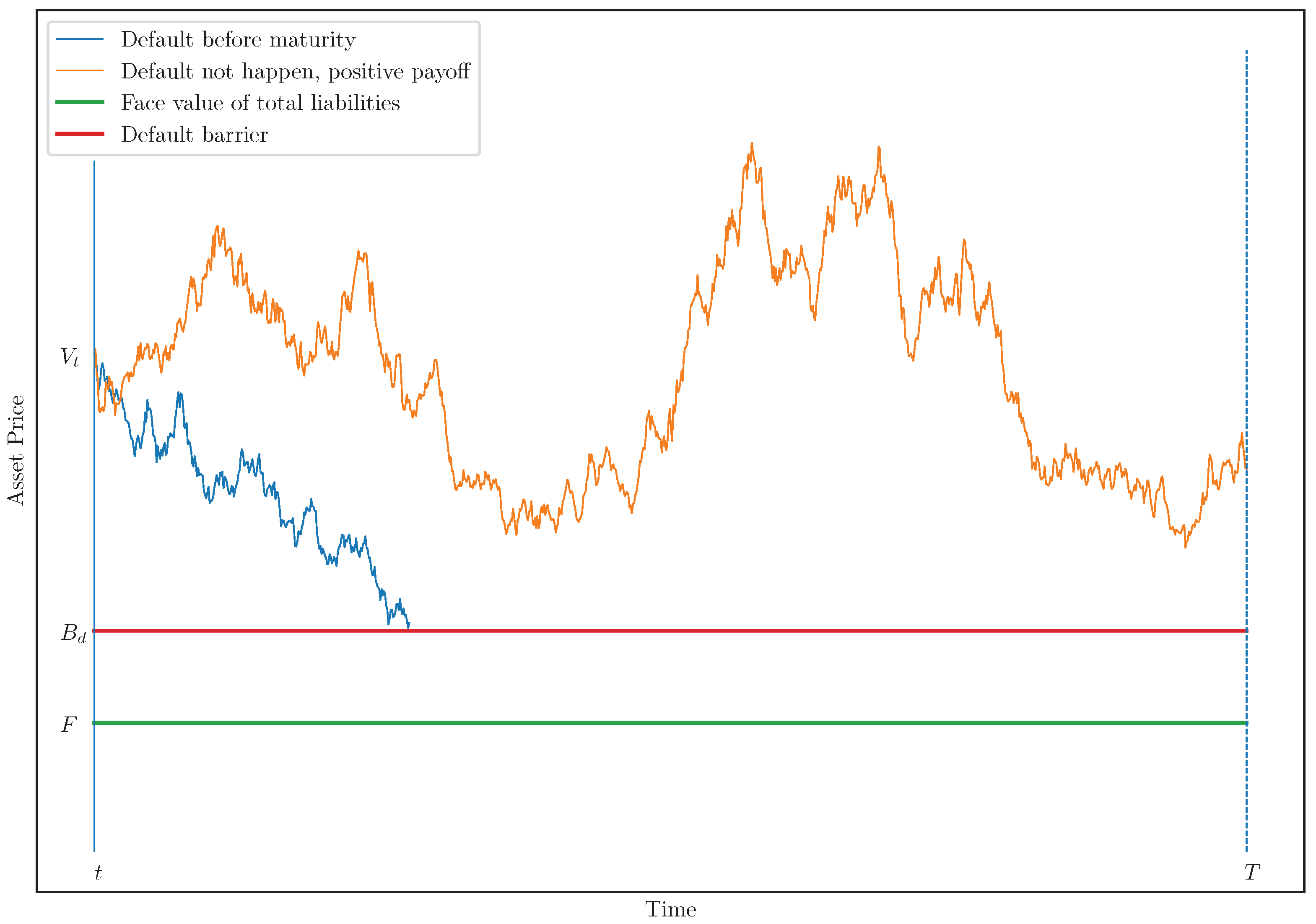
2.1. Firm–Value Model

Throughout this paper, we fix a probability space ($\Omega ,\mathcal{F},\mathbb{Q}$), with a filtration $\mathbb{F}={\left\{{\mathcal{F}}_t\right\}}_{t\ge 0}$ that represents the information generated by the bank’s asset value process. We assume that the market is arbitrage-free, and $\mathbb{Q}$ represents the corresponding risk-neutral pricing measure. Let $\mathbb{E}$ denote expectation with respect to $\mathbb{Q}$. The interest rate r is deterministic and independent of both time and tenor, such that $r>0$ and the term structure is flat. Lando (2009) discussed stochastic interest rates and found that the interest rates have to be very volatile to have a significant effect on credit spreads, supporting our assumption regarding the interest rate.

Let $V_t$ denote the time-t value of the bank’s assets. The non-negative process ${\left\{V_t\right\}}_{t\ge 0}$ is adapted to $\mathbb{F}$ such that the discounted gains process is a $\mathbb{Q}$ martingale. We assume $V_t$ follows a jump-diffusion process with dynamics:

$$\begin{array}{cc}\hfill \mathrm{d}{V}_t& =\left(r-q-\lambda \nu \right)V_{t^{-}}\mathrm{d}t+{\sigma }_V{V}_{t^{-}}\mathrm{d}{W}_t+(\Pi -1)V_{t^{-}}\mathrm{d}{N}_t,\hfill \end{array}$$

(1)

where q represents the payout ratio, ${\sigma }_V$ is the bank’s asset volatility, and both q and ${\sigma }_V$ are assumed constant over time. ${\left\{W_t\right\}}_{t\ge 0}$ is a standard Brownian motion, ${\left\{N_t\right\}}_{t\ge 0}$ is a Poisson process with intensity parameter $\lambda$, $\Pi >0$ is the jump amplitude with $\mathbb{E}[\Pi ]=\nu +1$, where $\nu$ is the expected percentage change in the asset value when a jump occurs, and the asset price V changes by $V·(\Pi -1)$. The Brownian motion ${\left\{W_t\right\}}_{t\ge 0}$, Poisson process ${\left\{N_t\right\}}_{t\ge 0}$, and the jump sizes are mutually independent. Both $\lambda$ and $\nu$ are non-negative parameters, and when $\lambda =0$, the process reduces to geometric Brownian motion (GBM).

We assume that the jump size $\Pi =e^Y$ follows a log-normal distribution, such that

$$\begin{array}{c}\hfill ln(\Pi )\sim N({\mu }_Y,{\sigma }_Y^2),\end{array}$$

(2)

where $N(\mu ,{\sigma }^2)$ refers to a normal distribution with mean $\mu$ and variance ${\sigma }^2$. Hence,

$$\begin{array}{cc}\hfill \nu & =\mathbb{E}\left[e^Y\right]-1=e^{{\mu }_Y+{\sigma }_Y^2/2}-1.\hfill \end{array}$$

(3)

In the interest of being conservative, we forced the vast majority of jumps to be negative by imposing the following relation between ${\mu }_Y$ and ${\sigma }_Y$, such that ${\sigma }_Y$ can be obtained once ${\mu }_Y$ is specified:

$$\begin{array}{c}\hfill \mathbb{P}\left(Z\le -\frac{{\mu }_Y}{{\sigma }_Y}\right)=0.9999,\end{array}$$

(4)

where $Z\sim N(0,1)$. This arbitrarily imposed relation between ${\mu }_Y$ and ${\sigma }_Y$ not only imposes negative jumps but also reduces the number of parameters to be calibrated.

2.2. Capital Structure Assumptions

Following two previous studies on Canadian banks, Beyhaghi et al. (2014) and Li (2015), we classified bank debt liabilities into three buckets based on their seniority: deposits, senior debt, and junior debt. We assume that liabilities have a common maturity of $T>0$ years. Default is defined as the event when the bank’s asset value first falls below the corresponding default barrier, and the default time is defined as the first time the asset value breaches the barrier. As demonstrated in Figure 1, we assume the default barrier $B_d$ does not vary through time. The bank will cease operations at $min({\tau }_d,T)$, where ${\tau }_d=inf\{t\in (0,T]:V_t\le B_d\}$ represents the default time; by convention, the infimum of an empty set is equal to infinity, such that if the default does not happen, ${\tau }_d=\infty$, the bank liquidates at time T and the debtholders are fully paid. We denote $B_d=d·F$ as the default barrier. The default threshold $d>1$ is expressed as a percentage of the total nominal liability $F=F_D+F_S+F_J$, where $F_j$ represents the nominal value of liability $j\in \{D,S,J\}$, and $D,S,J$ denote deposits, senior debt, and junior debt, respectively. The default threshold d is treated as a parameter to be calibrated.

Under the absolute priority rule, debts to creditors are paid off first, then equity holders divide any remaining assets. Creditors are paid based on seniority; for example, junior creditors do not receive any payment unless senior creditors are fully paid. Let ${\widehat{F}}_j$ be the payoff of debt at terminal time, ${\tau }_d\wedge T$, for $j\in \{D,S,J\}$. The absolute priority rule can be expressed by

$$\begin{array}{cc}\hfill {\widehat{F}}_D& =V_{{\tau }_d\wedge T}\wedge F_D,\hfill \end{array}$$

(5)

$$\begin{array}{cc}\hfill {\widehat{F}}_S& ={\left(V_{{\tau }_d\wedge T}-F_D\right)}^{+}-{\left(V_{{\tau }_d\wedge T}-F_D-F_S\right)}^{+},\mathrm{and}\hfill \end{array}$$

(6)

$$\begin{array}{cc}\hfill {\widehat{F}}_J& ={\left(V_{{\tau }_d\wedge T}-F_D-F_S\right)}^{+}-{\left(V_{{\tau }_d\wedge T}-F_D-F_S-F_J\right)}^{+}.\hfill \end{array}$$

(7)

Equations (5)–(7) assume there are no bankruptcy costs.

Weiss (1990) showed that the absolute priority rule of claims is rarely followed in practice as equity holders usually receive some compensation during bankruptcy and senior creditors are normally not fully paid. Hence, in this paper, we assume the absolute priority rule is not strictly followed. That is, the junior debt holders may receive payments without the senior debt holders being fully paid. Equity holders may also be compensated. We assume the following:

• The depositors are always paid fully, i.e., the recovery rate of deposits ${\mathcal{R}}_D$ is $100\%$. It is worth noting that deposits are normally fully insured by government agencies under a certain amount, such as the Federal Deposit Insurance Corporation (FDIC) in the United States and the Canada Deposit Insurance Corporation (CDIC) in Canada.6
• Both senior and junior debts are partially recovered, where the recovery rate of senior debt is higher than that of junior debt. We denote ${\mathcal{R}}_S$ and ${\mathcal{R}}_J$ as the recovery rate for senior and junior debt, respectively, and assume that ${\mathcal{R}}_S\ge {\mathcal{R}}_J$. The recovery rates are treated as unknown constants to be calibrated.
• We assume that the residual value at liquidation, $RV$, is split equally between equity holders and bankruptcy costs. $RV$ is defined as the difference between the bank’s asset value at default and the total amount paid to creditors:

  $$\begin{array}{cc}\hfill RV& =\left(V_{{\tau }_d}-({\mathcal{R}}_D{F}_D+{\mathcal{R}}_S{F}_S+{\mathcal{R}}_J{F}_J)\right){\mathbb{I}}_{\{{\tau }_d\le T\}}.\hfill \end{array}$$

  (8)

Remark 1.

To complete the definition of the residual value, we need to specify what happens when the bank’s asset value jumps below the sum of the recovered values, i.e., when $V_{{\tau }_d}<({\mathcal{R}}_D{F}_D+{\mathcal{R}}_S{F}_S+{\mathcal{R}}_J{F}_J)$ in Equation (8). For the parameter values in this paper, this event never occurred, so we are agnostic about the residual value in this case.

Remark 2.

Stochastic recovery rates are empirically observed, and these are built into certain models; for example, the Merton model. However, we were able to obtain acceptable calibration results without the added complexity of stochastic recovery rates.

In summary, we assume that the default payout is distributed to three parties: (1) liability holders, with total payout ${\mathcal{R}}_D{F}_D+{\mathcal{R}}_S{F}_S+{\mathcal{R}}_J{F}_J$, where ${\mathcal{R}}_D=100\%$, and ${\mathcal{R}}_J\le {\mathcal{R}}_S\le 100\%$; (2) equity holders, with payout $0.5·RV$; and (3) bankruptcy costs, with payout $0.5·RV$. We could introduce an additional parameter $\omega$, which dictates the proportion of residual value that leaves the bank in the form of bankruptcy costs, such that the bankruptcy costs are $(1-\omega )·RV$ when default occurs and equity holders receive $w·RV$, but we have not found that useful.

2.3. Valuation

In this section, we derived the valuation expressions for stock price, equity volatility, CDS spread, equity option price, and bond yields. These rely on valuation equations for the capital structure securities.

Two scenarios are considered: (1) when $\lambda =0$, the asset value dynamics reduce to geometric Brownian motion (GBM), and closed-form valuation expressions are derived, and (2) when $\lambda >0$, we approximated the valuation through simulation. The simulation steps are provided in Appendix C.

2.3.1. Debt Valuation

The time-t value of debt-j, $j\in \{D,S,J\}$, equals the summation of the present value of coupon payments received and the payoff at maturity or default,

$$\begin{array}{cc}\hfill L_t^j(V_t;B_d,T)& ={\mathbb{E}}_{t,V_t}\left[{\int }_t^{T\wedge {\tau }_d}\left(e^{-r(s-t)}{i}_j{F}_j\right)\mathrm{d}s+e^{-r(T-t)}{F}_j{\mathbb{I}}_{\{{\tau }_d=\infty \}}+e^{-r({\tau }_d-t)}{\mathcal{R}}_j{F}_j{\mathbb{I}}_{\{{\tau }_d\le T\}}\right],\hfill \end{array}$$

(9)

where $i_j$ represents the coupon rate of debt j, and ${\mathbb{E}}_{t,V_t}[·]$ denotes the time-t asset value-$V_t$ conditional expected value. Equation (9) evaluates debt in the context of all possible asset value processes. When we allow jumps, such that $\lambda >0$, the debt value is approximated through simulation, and the details are in Appendix C.

When the asset value evolves as GBM, Equation (9) can be evaluated following Leland and Toft (1996), such that the debt value with maturity T is:

$$\begin{array}{cc}\hfill L_t^j(V_t;B_d,T)& =\frac{i_j{F}_j}{r}+e^{-r(T-t)}\left[F_j-\frac{i_j{F}_j}{r}\right]\left(1-F_{{\tau }_d}(T-t)\right)+\left[{\mathcal{R}}_j{F}_j-\frac{i_j{F}_j}{r}\right]G(T-t),\hfill \end{array}$$

(10)

where $f_{{\tau }_d}\left(t\right)=f_{{\tau }_d}(t;V_t,B_d)$ is the probability density of the first passage time ${\tau }_d$ to $B_d$ from $V_t$ and $F_{{\tau }_d}\left(t\right)=F_{{\tau }_d}(t;V_t,B_d)$ is the corresponding cumulative distribution function, and

$$\begin{array}{cc}\hfill F_{{\tau }_d}(T-t)& =\mathcal{N}\left(h_1(T-t)\right)+{\left(\frac{V_t}{B_d}\right)}^{-2a}\mathcal{N}\left(h_2(T-t)\right),\hfill \end{array}$$

(11)

$$\begin{array}{cc}\hfill G(T-t)& ={\int }_t^T{e}^{-r(s-t)}{f}_{{\tau }_d}(t;V_t,B_d)\mathrm{d}s\hfill \\ \hfill & ={\left(\frac{V_t}{B_d}\right)}^{-a+z}\mathcal{N}\left(q_1(T-t)\right)+{\left(\frac{V_t}{B_d}\right)}^{-a-z}\mathcal{N}\left(q_2(T-t)\right),\hfill \end{array}$$

(12)

where $\mathcal{N}(·)$ is the standard normal cumulative distribution function and expressions for $h_1(T-t)$, $h_2(T-t)$, $q_1(T-t)$, $q_2(T-t)$, and a, z, $\delta$, $\gamma$ are provided in Appendix A. $G(T-t)$ represents the expected present value of the payoff received by the debtholders on the bond with a USD 1 face value if a default occurs.

2.3.2. Bankruptcy Costs

The bankruptcy costs can be expressed as

$$\begin{array}{cc}\hfill B{C}_t& ={\mathbb{E}}_{t,V_t}\left[\frac{1}{2}·e^{-r({\tau }_d-t)}·RV\right].\hfill \end{array}$$

(13)

With the additional assumption that the asset value evolves as GBM, we obtain

$$\begin{array}{cc}\hfill B{C}_t& =\frac{1}{2}·{\int }_t^T{e}^{-r(s-t)}\left(V_{{\tau }_d}-\sum _j{\mathcal{R}}_j{F}_j\right)f_{{\tau }_d}(s;V_t,B_d)\mathrm{d}s\hfill \\ \hfill & =\frac{1}{2}·\left(V_{{\tau }_d}-\sum _j{\mathcal{R}}_j{F}_j\right)·G(T-t),j\in \{D,S,J\}.\hfill \end{array}$$

(14)

The value of the bankruptcy cost is zero if ${\tau }_d>T$.7

2.3.3. Equity Valuation

The time-t equity value and share price can be expressed as

$$\begin{array}{cc}\hfill E_t& =g(t,V_t)=V_t-L_t-B{C}_t,\mathrm{and}\hfill \end{array}$$

(15)

$$\begin{array}{cc}\hfill S_t& =\frac{E_t}{N_S},\hfill \end{array}$$

(16)

respectively, where $N_S$ is the number of shares outstanding, $L_t={\sum }_j{L}_t^j$, and $j\in \{D,S,J\}$ is the time-t total value of liabilities.

2.3.4. Model-Implied Equity Volatility

As shown in Equation (15), the equity value is a function of time and the bank’s asset value. We derived the model-implied equity volatility by applying Itô’s formula to Equation (15), where the jumps follow a compound Poisson process:

$$\begin{array}{cc}\hfill \mathrm{d}{E}_t& =\mathrm{d}g(t,V_t)\hfill \end{array}$$

(17)

$$\begin{array}{cc}\hfill & =\left(g_t+g_V{V}_{t^{-}}(r-q-\lambda \nu )+\frac{1}{2}{g}_{VV}{\sigma }_V^2{V}_{t^{-}}^2\right)\mathrm{d}t+g_V{\sigma }_V{V}_{t^{-}}\mathrm{d}{W}_t+\Delta g\mathrm{d}{N}_t,\hfill \end{array}$$

(18)

where $\Delta g=g(t,V_{t^{-}}·(\Pi -1))-g(t,V_{t^{-}})$, $g_t=\frac{\partial }{\partial t}g(t,V_t)$, $g_V=\frac{\partial }{\partial V_t}g(t,V_t)$, and $g_{VV}=\frac{{\partial }^2}{\partial V_t^2}g(t,V_t)$.

We defined

$$\begin{array}{c}\hfill {\sigma }_E(t,V)=g_V{\sigma }_{V}V\end{array}$$

(19)

as the diffusive component of equity volatility and

$$\begin{array}{cc}\hfill {\beta }_E(t,V)& =\sqrt{\lambda {\int }_0^{\infty }{[g(t,V·(e^y-1))-g(t,V)]}^2{f}_Y\left(y\right)\mathrm{d}y}\hfill \end{array}$$

(20)

as the jump component of equity volatility, where $f_Y\left(y\right)$ is the PDF of the random variable Y.

When there is no jump component, ${\beta }_E(t,V)=0$, and the diffusive component of equity volatility is given by

$$\begin{array}{cc}\hfill {\sigma }_E(t,V_t)& ={\sigma }_V\left(1-\mathcal{A}{G}_{V_t}^{\prime }+\mathcal{B}{F}_{V_t}^{\prime }-\mathcal{C}{G}_{V_t}^{\prime }\right)V_t.\hfill \end{array}$$

(21)

It can be shown that the standard deviation of the daily log return on equity over time interval $(t,t+h)$ is approximately $\sqrt{h}{\sigma }_E(t,V_t)/E_t$. The derivation of Equation (21) and the expressions for $\mathcal{A}$, $\mathcal{B}$, $\mathcal{C}$, $G_{V_t}^{\prime }$, and $F_{V_t}^{\prime }$ are detailed in Appendix B.

When $\lambda >0$, there is no closed-form solution for $g(t,V_t)$ and its derivatives, making it challenging to compute both the diffusive and jump components to equity volatility. Thus, we approximated the equity volatility through simulation. Our simulation result suggests that the variance of the log return on equity prices over time interval $(t,t+h)$ is proportional to the length of the time interval h:

$$\begin{array}{cc}\hfill \mathrm{Var}\left(ln\left(\frac{E_{t+h}}{E_t}\right)\right)& =\frac{{\sigma }_E^2(t,V_t)+{\beta }_E^2(t,V_t)}{E_t}·h+o\left(h\right).\hfill \end{array}$$

(22)

This result ensures that we can compare the model-implied equity volatility with the market-observed equity volatility, computed as the standard deviation of historical daily log returns (annualized). Thus, the model-implied equity volatility can be approximated by

$$\begin{array}{cc}\hfill \sqrt{\frac{{\sigma }_E^2(t,V_t)+{\beta }_E^2(t,V_t)}{E_t}}& \approx \mathrm{SD}\left(\frac{ln\left(E_{t+h}/E_t\right)}{\sqrt{h}}\right).\hfill \end{array}$$

(23)

Thus, for the jump-diffusion model, we approximated the model-implied equity volatility using

$$\begin{array}{cc}\hfill \sqrt{\frac{{\sigma }_E^2(t,V_t)+{\beta }_E^2(t,V_t)}{E_t}}& \approx \mathrm{SD}\left(\frac{ln\left(E_{T\wedge {\tau }_d}/E_t\right)}{\sqrt{T\wedge {\tau }_d-t}}\right),\hfill \end{array}$$

(24)

where the right-hand side is estimated by simulation (see Appendix C).

2.3.5. CDS Spread

A credit default swap (CDS) is an insurance contract that pays off if a particular company or country defaults. The company or country is known as the reference entity. The buyer of credit protection pays an insurance premium, known as the CDS spread, to the seller of protection for the life of the contract or until the reference entity defaults (Hull (2018) and Hull and White (2000)). As the simplest contract, a single-name CDS covers the risk if the reference entity defaults. Following the reference entity default event, the buyer of the CDS receives a payment from the seller to compensate for credit losses (see Amato and Gyntelberg (2005)).

The protection leg–also known as the default leg or the contingent leg–is the payment that the seller makes to the buyer upon default. The premium leg refers to the payments made by the buyer to the seller (see Metzler (2008)). The amount that the protection seller pays out if a credit event is triggered is referred to as the contingent leg. Assume the CDS is on the senior debt and let $s_t$ denote the CDS spread at time t, then $s_t$ is set to equate the premium and contingent legs, leading to

$$\begin{array}{cc}\hfill (1-{\mathcal{R}}_S){\mathbb{E}}_{t,V_t}\left[e^{-r({\tau }_d-t)}{\mathbb{I}}_{\{{\tau }_d\le T\}}\right]& =s_t{\int }_t^T{e}^{-r(u-t)}{\mathbb{E}}_{t,V_t}\left[{\mathbb{I}}_{\{{\tau }_d>u\}}\right]\mathrm{d}u,\hfill \end{array}$$

(25)

giving

$$\begin{array}{cc}\hfill s_t& =\frac{r(1-{\mathcal{R}}_S){\mathbb{E}}_{t,V_t}\left[e^{-r({\tau }_d-t)}{\mathbb{I}}_{\{{\tau }_d\le T\}}\right]}{1-{\mathbb{E}}_{t,V_t}\left[e^{-r({\tau }_d\wedge T-t)}\right]}.\hfill \end{array}$$

(26)

When the asset value process evolves as GBM, Equation (26) simplifies to

$$\begin{array}{cc}\hfill s_t& =\frac{r(1-{\mathcal{R}}_S)G(T-t)}{1-G(T-t)-e^{-r(T-t)}[1-F_{{\tau }_d}(T-t)]},\hfill \end{array}$$

(27)

with $F_{{\tau }_d}(T-t)$ and $G(T-t)$ defined in Equations (11) and (12), respectively.

2.3.6. Equity Option Valuation

The equity option, written on the firm share price, can be viewed as a down-and-out compound option with a barrier. Following Geske (1979), Geske et al. (2016), Zhou (2018), and Campolieti and Makarov (2018), let $T_o$ be the maturity time of the equity call option, with a strike price K,8 and the time-t (European) call option price can be expressed as

$$\begin{array}{cc}\hfill C_t& ={\mathbb{E}}_{t,S_t}\left[e^{-r(T_o-t)}{\left(S_{T_o}-K\right)}^{+}{\mathbb{I}}_{\{{\tau }_d>T_o\}}{S}_t\right]\hfill \\ \hfill & =e^{-r(T_o-t)}{\mathbb{E}}_{t,S_t}\left[\left(S_{T_o}-K\right){\mathbb{I}}_{\{{\tau }_d>T_o,S_{T_o}>K\}}\right],\hfill \end{array}$$

(28)

where ${\mathbb{E}}_{t,S_t}[·]$ denotes the time-t and stock price-$S_t$ conditional expected value. Note that the option payoff is positive if, and only if, a default does not happen before the option matures, and the time-$T_o$ stock price is greater than the strike price K.

We denote the realized minimum asset value on the interval [$t,T_o$] as

$$\begin{array}{c}\hfill m\left(T_o\right)\equiv m^V\left(T_o\right):=\underset{t\le u\le T_o}{\inf }{V}_u.\end{array}$$

(29)

Then, we have the equivalence of events:

$$\begin{array}{c}\hfill \{m\left(T_o\right)>B_d\}=\{{\tau }_d>T_o\},\end{array}$$

(30)

such that a default does not occur before $T_o$, and the value of the call option is equivalent to

$$\begin{array}{cc}\hfill C_t& =e^{-r(T_o-t)}{\mathbb{E}}_{t,S_t}\left[\left(S_{T_o}-K\right){\mathbb{I}}_{\{m\left(T_o\right)>B_d,S_{T_o}>K\}}\right]\hfill \\ \hfill & =e^{-r(T_o-t)}{\mathbb{E}}_{t,V_t}\left[\left(\frac{g(T_o,V_{T_o})}{N_S}-K\right){\mathbb{I}}_{\{m\left(T_o\right)>B_d,V_{T_o}>V^{*}\}}\right],\hfill \end{array}$$

(31)

where $S_{T_o}=E_{T_o}/N_S=g\left(V_{T_o}\right)/N_S$, $N_S$ is the number of shares outstanding, and $V^{*}$ solves $g(T_o,V_{T_o})=K{N}_S$.9

When the asset value evolves as jump-diffusion, we approximated Equation (31) using simulation, and the simulation steps are in Appendix C. When the asset value evolves as GBM, Equation (31) simplifies to

$$\begin{array}{cc}\hfill C_t& =e^{-r(T_o-t)}{\int }_{V^{*}}^{\infty }\left(\frac{g(T_o,v)}{N_S}-K\right)f_{V_{T_o}}\left(v\right)\mathrm{d}v,\hfill \end{array}$$

(32)

where

$$\begin{array}{cc}\hfill f_{V_{T_o}}\left(v\right)& =\frac{1}{v{\sigma }_V\sqrt{T_o-t}}\left[n\left(\frac{ln\frac{V_t}{v}+\mu (T_o-t)}{{\sigma }_V\sqrt{T_o-t}}\right)-{\left(\frac{B_d}{V_t}\right)}^{\frac{2\mu }{{\sigma }_V^2}}n\left(\frac{ln\frac{B_d^2}{v{V}_t}+\mu (T_o-t)}{{\sigma }_V\sqrt{T_o-t}}\right)\right],\hfill \end{array}$$

(33)

$$\begin{array}{cc}\hfill g(T_o,V_{T_o})& =E_{T_o}=V_{T_o}-\sum _j{L}_j(V_{T_o};B_d,T-T_o)-B{C}_{T_o}\hfill \\ \hfill & =V_{T_o}-\sum _j\left[\frac{i_j{F}_j}{r}+e^{-r\overline{T}}\left(F_j-\frac{i_j{F}_j}{r}\right)\left(1-F_{{\tau }_d}\left(\overline{T}\right)\right)+\left({\mathcal{R}}_j{F}_j-\frac{i_j{F}_j}{r}\right)G\left(\overline{T}\right)\right]\hfill \\ \hfill & -\frac{1}{2}\left(B_d-\sum _j{\mathcal{R}}_j{F}_j\right)·G\left(\overline{T}\right),\hfill \end{array}$$

(34)

where $\overline{T}=T-T_o$, $f_{V_{T_o}}\left(v\right)$ is the transition density of the asset value process starting at $V_t$ and ending at v conditioned on not hitting the default barrier $B_d$ between time-t and $T_o$, $g(T_o,V_{T_o})$ represents the equity value at time $T_o$ as a function of the asset value at $T_o$, and $n(·)$ is the standard normal probability density function.

2.3.7. Debt Yield

For debt with face value $F_j$, its corresponding yield, $y_j$, is determined by solving the equation below:

$$\begin{array}{cc}\hfill F_j·{\int }_t^T{i}_j·e^{-y_{j}u}\mathrm{d}u+e^{-y_j(T-t)}& =L_t^j,\hfill \end{array}$$

(35)

where $F_j$ is the face value of the debt, $L_t^j$ is the time-t value of the debt, defined in Equation (9), and $i_j$ represents the coupon rate of debt j, where $j\in \{S,J\}$. Since the deposits are assumed to be fully recovered, the yield of deposits is the risk-free rate. When the asset value evolves as GBM ($\lambda =0$), the time-t debt value is expressed in Equation (10), and we determined the yield through Equation (35).

On the other hand, when jumps are allowed in the model ($\lambda >0$), we employed simulation for debt yield estimation. Note that it is time-consuming to determine the debt yield using simulation. To avoid this, we approximated the true yield with the yield on an otherwise identical zero-coupon bond.10 Hence, Equation (35) simplifies to

$$\begin{array}{cc}\hfill e^{-y_j(T-t)}& ={\mathbb{E}}_{t,V_t}\left[e^{-r(T-t)}{\mathbb{I}}_{\{{\tau }_d>T\}}+e^{-r({\tau }_d-t)}{\mathcal{R}}_j{\mathbb{I}}_{\{{\tau }_d\le T\}}\right],\hfill \end{array}$$

(36)

which is equivalent to

$$\begin{array}{cc}\hfill y_j& =-\frac{1}{T-t}{\mathbb{E}}_{t,V_t}\left[ln\left(e^{-r(T-t)}-e^{-r(T-t)}\left[(1-{\mathcal{R}}_j){\mathbb{I}}_{\{{\tau }_d\le T\}}\right]\right)\right].\hfill \end{array}$$

(37)

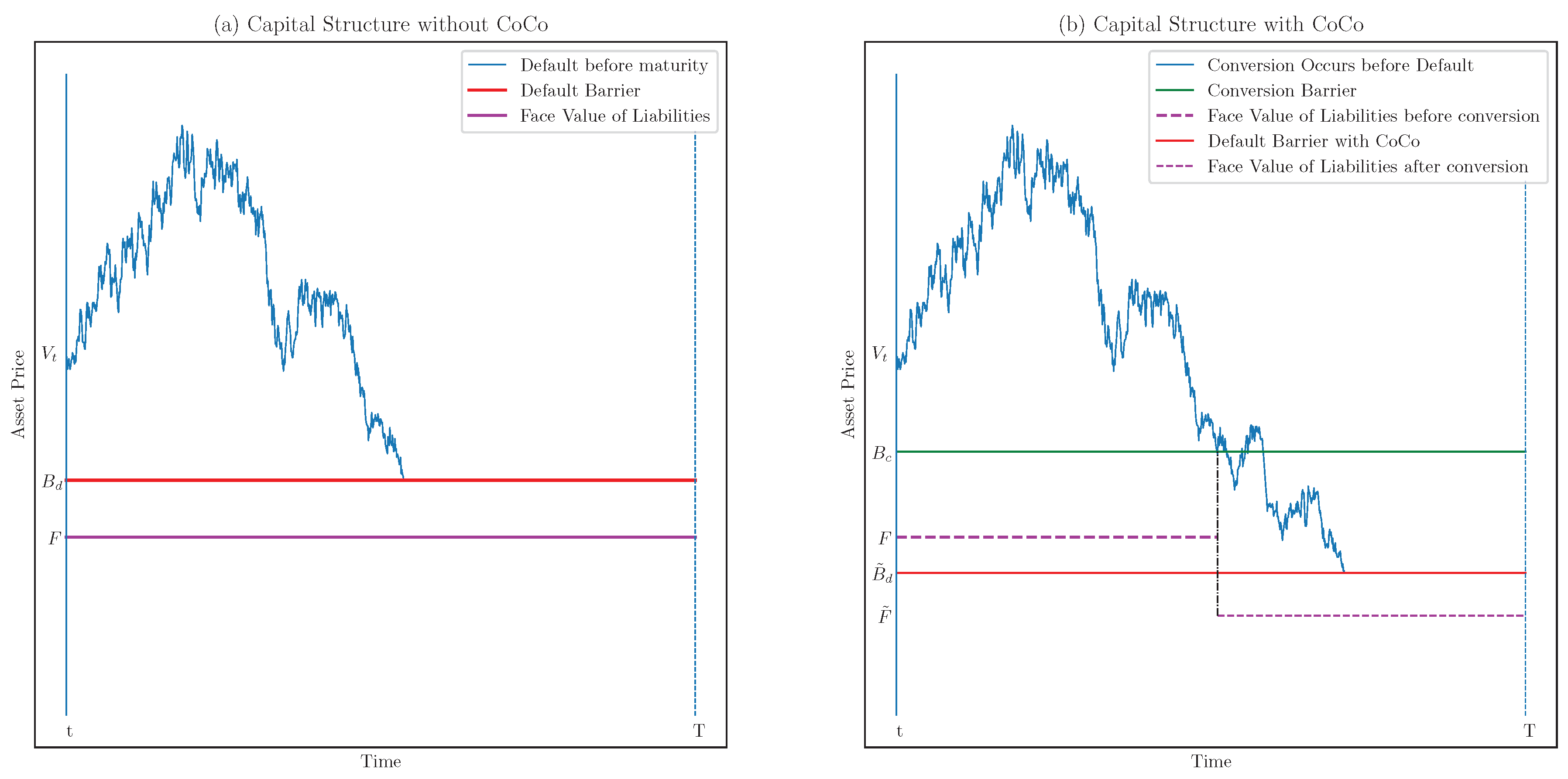
3. Capital Structure with Contingent Capital

We now consider a bank that replaces the junior debt with a contingent convertible security (CoCo), such that the bank’s liabilities consist of (1) deposits, (2) senior debt, and (3) CoCo. We assume that the coupon rate $i_{CC}$, face value $F_{CC}$, and tenor of the CoCo are the same as those of the junior debt.

3.1. Assumptions

Figure 2 demonstrates the mechanism of CoCo and the leverage decrease that occurs at CoCo conversion. As described in Section 2, if there is no CoCo in the capital structure, such as in Figure 2a, the bank enters bankruptcy when its asset value process reaches the default barrier $B_d$. With CoCo in the capital structure, on the other hand, the key assumptions and features are as follows:

• We assume that conversion is triggered when the bank’s asset–liability ratio falls below a pre-specified level c, defined as $B_c=cF$, where $B_c$ is the conversion barrier, assumed to be constant over time, and the conversion threshold c is expressed as a percentage of the face value of total liabilities F.
• A main goal of this paper is to use market-observed data to infer the exogenous conversion threshold c.
• Upon conversion, the bank’s liabilities are reduced from F to $F-F_{CC}$, and we assume that default occurs upon the first passage of asset value to the level $d·(F-F_{CC})$ and $cF>d·(F-F_{CC})$, or $c>d·(1-F_{CC}/F)$.
• As illustrated in Figure 2b, incorporating CoCo instruments would delay the time of default when compared to the scenario where the bank did not issue any CoCos, as in Figure 2a.

Denote $N_S^{*}$ as the number of newly issued common shares distributed to the CoCo holders upon conversion. Also upon conversion, the CoCo holders become $100w\%$ owners of the bank, where $w=N_S^{*}/(N_S^{*}+N_S)$. Note that, in general, both $N_S^{*}$ and w are stochastic whose values are not necessarily determined prior to conversion. However, there is the reasonable assumption that both variables are ${\mathcal{F}}_{{\tau }_c}$-measurable, where ${\tau }_c=\{t\in (0,T]:V_t\le B_c\}$ represents the conversion time. Similar to the rules determining the default time in Section 2, the infimum of the empty set is equal to infinity, and $N_S^{*}$ and w are determined upon conversion.

We assume that CoCo investors lose a certain percentage of face value on the debt when the conversion occurs. Denote l as the percentage loss, where $l\in (0,1)$, and we have

$$\begin{array}{cc}\hfill N_S^{*}& =\frac{(1-l)F_{CC}}{S_{{\tau }_c}}=\frac{F_{CC}}{{(1-l)}^{-1}{S}_{{\tau }_c}},\hfill \end{array}$$

(38)

where we may interpret $S_{{\tau }_c}^{*}={(1-l)}^{-1}{S}_{{\tau }_c}$ as a conversion price of the CoCo. With this interpretation, the conversion price is proportional to the bank’s stock price at conversion, and we would call ${(1-l)}^{-1}$ the multiplier. A more rigorous discussion on CoCo can be found in Metzler and Reesor (2015).

3.2. Valuation

In this section, we discuss valuation expressions for debt and equity at time-t and conversion time ${\tau }_c$, where $t<{\tau }_c\le {\tau }_d$11. We start with the time-${\tau }_c$ value of deposits, senior bonds, and bankruptcy costs:

$$\begin{array}{cc}\hfill L_{{\tau }_c}^D& ={\mathbb{E}}_{{\tau }_c,V_{{\tau }_c}}\left[\left(e^{-r(T-{\tau }_c)}{F}_D+{\mathrm{CP}}_{{\tau }_c,T}^D\right){\mathbb{I}}_{\{{\tau }_d=\infty \}}+\left(e^{-r({\tau }_d-{\tau }_c)}{\mathcal{R}}_D{F}_D+{\mathrm{CP}}_{{\tau }_c,{\tau }_d}^D\right){\mathbb{I}}_{\{{\tau }_d\le T\}}\right],\hfill \end{array}$$

(39)

$$\begin{array}{cc}\hfill L_{{\tau }_c}^S& ={\mathbb{E}}_{{\tau }_c,V_{{\tau }_c}}\left[\left(e^{-r(T-{\tau }_c)}{F}_S+{\mathrm{CP}}_{{\tau }_c,T}^S\right){\mathbb{I}}_{\{{\tau }_d=\infty \}}+\left(e^{-r({\tau }_d-{\tau }_c)}{\mathcal{R}}_S{F}_S+{\mathrm{CP}}_{{\tau }_c,{\tau }_d}^S\right){\mathbb{I}}_{\{{\tau }_d\le T\}}\right],\hfill \end{array}$$

(40)

$$\begin{array}{cc}\hfill B{C}_{{\tau }_c}& ={\mathbb{E}}_{{\tau }_c,V_{{\tau }_c}}\left[\frac{1}{2}{e}^{-r({\tau }_d-{\tau }_c)}{\left(V_{{\tau }_d}-{\mathcal{R}}_D{F}_D-{\mathcal{R}}_S{F}_S\right)}^{+}{\mathbb{I}}_{\{{\tau }_d\le T\}}\right],\hfill \end{array}$$

(41)

where

$$\begin{array}{c}\hfill {\mathrm{CP}}_{t_1,t_2}^j={\int }_{t_1}^{t_2}\left(e^{-r(s-t_1)}{i}_j{F}_j\right)\mathrm{d}s\end{array}$$

(42)

denotes the time-$t_1$ value of the continuously received coupon between time $t_1$ and $t_2$ for investors of debt $j\in \{D,S,CC\}$.

Denote the residual value at conversion $R_{{\tau }_c}$ as12

$$\begin{array}{cc}\hfill R_{{\tau }_c}& ={(V_{{\tau }_c}-L_{{\tau }_c}^D-L_{{\tau }_c}^S-B{C}_{{\tau }_c})}^{+}.\hfill \end{array}$$

(43)

Note that the residual values are defined slightly differently between the case with CoCo and without CoCo in the capital structure. Upon conversion, CoCo holders receive $100w\%$ of the bank’s equity, where

$$\begin{array}{cc}\hfill w& =\min \left(1,\frac{(1-l)F_{CC}}{R_{{\tau }_c}}\right).\hfill \end{array}$$

(44)

Note that $w{R}_{{\tau }_c}$ denotes the market value of the equity received at conversion and is equal to the minimum of (i) $(1-l)F_{CC}$, in which case the debt is redeemed at $100(1-l)\%$, and (ii) $R_{{\tau }_c}$. Thus, the time-${\tau }_c$ value of CoCo13 is

$$\begin{array}{cc}\hfill L_{{\tau }_c}^{CC}& =w{R}_{{\tau }_c}.\hfill \end{array}$$

(45)

Prior to conversion, the time-t values are

$$\begin{array}{cc}\hfill L_t^D& ={\mathbb{E}}_{t,V_t}\left[\left(e^{-r(T-t)}{F}_D+{\mathrm{CP}}_{t,T}^D\right){\mathbb{I}}_{\{{\tau }_c=\infty \}}+\left(e^{-r({\tau }_c-t)}{L}_{{\tau }_c}^D+{\mathrm{CP}}_{t,{\tau }_c}^D\right){\mathbb{I}}_{\{{\tau }_c\le T\}}\right]\hfill \end{array}$$

(46)

$$\begin{array}{cc}\hfill L_t^S& ={\mathbb{E}}_{t,V_t}\left[\left(e^{-r(T-t)}{F}_S+{\mathrm{CP}}_{t,T}^S\right){\mathbb{I}}_{\{{\tau }_c=\infty \}}+\left(e^{-r({\tau }_c-t)}{L}_{{\tau }_c}^S+{\mathrm{CP}}_{t,{\tau }_c}^S\right){\mathbb{I}}_{\{{\tau }_c\le T\}}\right]\hfill \end{array}$$

(47)

$$\begin{array}{cc}\hfill L_t^{CC}& ={\mathbb{E}}_{t,V_t}[\left(e^{-r(T-t)}{F}_{CC}+{\mathrm{CP}}_{t,T}^{CC}\right){\mathbb{I}}_{\{{\tau }_c=\infty \}}+\left(e^{-r({\tau }_c-t)}{\mathcal{R}}_J{F}_{CC}+{\mathrm{CP}}_{t,{\tau }_c}^{CC}\right){\mathbb{I}}_{\{{\tau }_c={\tau }_d\le T\}}\hfill \\ \hfill & +\left(e^{-r({\tau }_c-t)}{L}_{{\tau }_c}^{CC}+{\mathrm{CP}}_{t,{\tau }_c}^{CC}\right){\mathbb{I}}_{\{{\tau }_c\le T,{\tau }_c\ne {\tau }_d\}}].\hfill \end{array}$$

(48)

Under the jump-diffusion model, there is a possibility that the process jumps over the conversion and default barriers simultaneously; CoCo conversion does not occur and the bank enters default.14

Finally, the time-t value of the bank’s original equity $E_t$ and the corresponding per share price $S_t$ are

$$\begin{array}{cc}\hfill E_t& =V_t-L_t^D-L_t^S-L_t^{CC},\mathrm{and}\hfill \end{array}$$

(49)

$$\begin{array}{cc}\hfill S_t& =\frac{E_t}{N_S},\hfill \end{array}$$

(50)

respectively. The capital structure securities and stock prices are approximated through simulation for the jump-diffusion model (see Appendix D).

4. Data

The data used in this paper are for the Big Five Canadian banks for fiscal year 2019, ending on October 31, 2019. For the risk-free interest rate, we approximate the risk-free rate using the yield of Canadian government one-year treasury bills on 31 October 2019, which is 1.76%, continuously compounded (following Hull (2018)). Alternatively, we can take the average yield of one-year treasury bills from 31 October 2018 to 31 October 2019. The yield during this period is relatively stable, quite close to the yield on 31 October 2019. The risk-free interest rates are obtained from Thomson-Reuters Datastream.

Table 1. Data of Big Five Canadian banks at the end of fiscal year 2019. The details of the variables are described in Section 4.

Panel A: Capital Structure (in millions)
Bank	BMO	CIBC	RBC	BNS	TD
Deposits	568,143	485,712	886,005	733,390	913,862
Senior Debt	221,338	122,563	439,064	263,546	383,741
Junior Debt	16,328	7574	25,948	22,917	35,786
Total Debt (Senior + Junior)	237,666	130,137	465,012	286,463	419,527
Total Liabilities	805,809	615,849	1,351,017	1,019,853	1,333,389
Equity (Market Cap)	61,363	47,175	145,741	83,658	129,521
Total Assets	867,172	663,024	1,496,758	1,103,511	1,462,910
Panel B: Capital Structure by Proportion
Bank	BMO	CIBC	RBC	BNS	TD
Deposits/Total Assets	65.52%	73.26%	59.19%	66.46%	62.47%
Senior Debt/Total Assets	25.52%	18.49%	29.33%	23.88%	26.23%
Junior Debt/Total Assets	1.88%	1.14%	1.73%	2.08%	2.45%
Equity/Total Assets	7.08%	7.12%	9.74%	7.58%	8.85%
Panel C: Payout Ratios
Bank	BMO	CIBC	RBC	BNS	TD
Interest Rate of Deposits	1.52%	1.73%	1.47%	1.89%	1.50%
Coupon Rate of Debts	3.90%	2.45%	3.20%	1.16%	2.70%
Dividend Yield	0.30%	0.38%	0.39%	0.39%	0.36%
Total Payout Ratio	1.85%	1.92%	1.85%	1.82%	1.61%
Panel D: Volatility, Yield, Spread, Stock, and Option
Bank	BMO	CIBC	RBC	BNS	TD
Equity Volatility	16.35%	17.06%	16.58%	17.47%	16.14%
Time-to-maturity of Liabilities (year)	5.63	4.21	6.03	6.47	3.68
Senior Debt Yield	2.17%	2.08%	2.26%	2.25%	2.15%
Junior Debt Yield	2.37%	2.28%	2.46%	2.45%	2.35%
CDS Spread	0.56%	0.47%	0.60%	0.73%	0.33%
Stock Price (CAD)	97.50	112.31	106.24	75.54	75.21
Option Price (CAD)	9.7	12.95	11.3	17.75	9.6
Option Strike Price (CAD)	90	100	96	58	66
Option Maturity (year)	0.96	0.55	0.55	0.55	0.55

reports the bank-specific data collected from various sources.

Capital structure data: Panel A reports the capital structure data, including the face value of deposits, senior and junior debt, total liabilities, equity value (market cap), and total assets. As described in Section 2 and Section 3, we assume the banks issue three types of liabilities: deposits, senior debt, and junior debt/CoCo. All equities are assumed to be common equity.

For the largest Canadian banks, deposits account for the largest part of the capital structure, between 60% and 75% of total assets. Thus, the inclusion of deposits can more accurately reflect the capital structure of these banks.

Li (2015) assigned senior secured debt and senior unsecured debt as senior debt and subordinated debt, preferred shares, and non-controlling interests as junior debt/CoCo. Here, we follow the same assignment as Li (2015), with additional assumptions. In the case of the Big Five Canadian banks, about 10% of liabilities cannot be classified into any bucket. These liabilities, including pension liabilities, deferred tax, derivative liabilities, other liabilities, etc., are too sizable to be ignored. Thus, in this paper, we assign these liabilities proportionally into senior debt and junior debt. Bloomberg provides a quarterly report on the aggregate proportion of senior secured and unsecured debt in relation to the total debt. We utilize this ratio to determine the percentage of total debt categorized as senior debt, while the remainder of liabilities, along with preferred shares, is designated as junior debt/CoCo.15

All data on liabilities are obtained from Bloomberg. Total debt is the summation of senior and junior debt, and when deposits are included, it results in the total liabilities. The equity values, i.e., equity (market cap), are obtained from the Center for Research in Security Prices, LLC (CRSP), computed as the fiscal year-end stock price multiplied by the shares outstanding, and the total assets are computed as the summation of the total liabilities and market cap of equity.

Capital structure by proportion: Panel B displays the share of deposits, senior debt, junior debt, and equity as a proportion of total assets. The results are computed based on Panel A.

Payout ratios: The payout ratios are presented in Panel C. We distinguish between interest and coupon payouts, where the interest payout refers to the payout made to the deposit holders only and the coupon payout represents the payout made to either senior or junior debtholders. Thus, total payouts include (1) interest payments to deposit holders, (2) coupon payments to senior debtholders, (3) coupon payments to junior debt (CoCo) holders, and (4) dividend payments to equity holders. We assume that all payouts are made continuously.

Bloomberg reports the total interest paid to the deposit holders and the total coupon paid to debtholders, without distinguishing between senior and junior holders. The interest rate on deposits is calculated by dividing the total interest paid by the deposit amount. The coupon rate of debts is a weighted average of both senior and junior debt, computed by dividing the total coupon payment by the total debt amount. To compute the respective senior and junior coupon rates, we assume that the coupon rate of junior debt is 20 basis points higher than the senior rate.

We compute the dividend yield following the methodology in Li (2015). The dividend yield, or dividend payout ratio at time t, is computed as the average of the previous ten years’ dividend yield, i.e.,

$$\begin{array}{c}\hfill di{v}_t=\frac{1}{10}\sum _{i=t-10}^{t-1}\frac{\mathrm{Cash}{\mathrm{Dividend}}_i}{\mathrm{Asset}{\mathrm{Value}}_i}.\end{array}$$

(51)

Both the cash dividend amount and the asset value are from Compustat-Capital IQ of Wharton Research Data Services (WRDS).

Thus, the time-t total payout ratio is

$$\begin{array}{cc}\hfill q·V_t& =\sum _j{i}_j{F}_j+di{v}_t·V_t,\hfill \end{array}$$

(52)

giving

$$\begin{array}{cc}\hfill q& =\sum _j\frac{i_j{F}_j}{V_t}+di{v}_t,\hfill \end{array}$$

(53)

and we assume it is constant across time. The value of q is determined at the initial time $t=0$.

Volatility, yield, CDS spread, stock, and equity option data: Panel D reports the value of equity volatility, senior and junior debt yield, CDS spread, the time-to-maturity of liabilities and CDS contracts, stock price, equity option price, strike price, and time-to-maturity for options.

We use the daily log returns to compute the equity volatility. The data are obtained from CRSP and are adjusted for dividends and stock splits. The time-t equity volatility is computed as the annualized standard deviation of previous 5-year returns, continuously compounded.

We assume that all liabilities (as well as the CDS contract) have the same time-to-maturity; Bloomberg provides the weighted average of the time-to-maturity for all debts (excluding deposits).

The senior debt yield is obtained from Bloomberg. We assume that each bank issues only one senior debt. Bloomberg reports a yield-to-maturity index for the senior debt of each bank on any given trading day, similar to the yield curve. Thus, the yield is computed by the linear interpolation of the yields of the nearest tenors. For example, in the case of BMO, the time-to-maturity for liabilities is 5.63 years and the 5-year and 7-year senior debt yields are $2.13\%$ and $2.26\%$, respectively. Interpolating the yield curve, the senior debt yield for the debt maturing in 5.63 years is approximately $2.17\%$.

The yield of junior debt under a non-contingent framework, however, is not directly observable in any of the data sources that we can access. Thus, we follow the results of Beyhaghi et al. (2014) and assume that the junior debt yield is 20 basis points higher than the corresponding senior debt yield. Similarly, we assume that each bank issues only one junior debt, with the maturity time the same as that of senior debt.

We assume that for each bank there is a single-name CDS contract on its senior debt. Similar to the senior debt yield, we source the CDS spread data from Bloomberg, which provides a curve of CDS spreads for any given trading day, with tenors ranging from 6 months to 10 years. Consequently, we calculate the CDS spread by linearly interpolating the spreads of the nearest tenors.

The stock prices at fiscal year-end are from CRSP and the data for equity options are from Datastream, where only in-the-money call options are considered, such that the option contract chosen has a strike price not higher than the stock price and the time-to-maturity is between half a year and one year. We exclude the option contracts that have zero trading volumes on 31 October 2019, and rank the strike prices of the remaining contracts, and choose the median as the strike price. If there are multiple contracts (at different maturities) with that strike price, we choose the one with the smallest bid-ask spread. For the options selected, we use the ask price at close on 31 October 2019.16 Note that the traded equity options are American style, though we treat them as European style here.

5. Calibration and Results

In this section, we calibrate the unknown parameters. The calibration includes two parts:

• Capital structure without CoCo: The parameters to be calibrated include the default threshold d, asset volatility ${\sigma }_V$, recovery rates for senior debt ${\mathcal{R}}_S$ and junior debt ${\mathcal{R}}_J$, and the average jump size ${\mu }_Y$ and jump frequency $\lambda$ under the jump-diffusion model. The reasons we start with no CoCos in capital structure are as follows:

  (1)

  To provide insights for the banks that only have regular debts in their capital structure.

  (2)

  Chen et al. (2013) showed that as long as conversion precedes default, the optimal default threshold remains unaffected by the conversion trigger. This forms the basis for incorporating these calibrated parameters when introducing CoCo instruments into the capital structure.

• Capital structure with CoCo: using the parameter values from Step 1, we then calibrate the conversion threshold, which is the only unknown parameter.

5.1. Non-Contingent Capital Structure

5.1.1. Calibration

The calibration is conducted by minimizing the loss function below:

$$\begin{array}{cc}\hfill \mathcal{L}& =\mathrm{argmin}\left[{\left(\frac{{\widehat{S}}_t}{S_t}-1\right)}^2+{\left(\frac{{\widehat{\sigma }}_E}{{\sigma }_E}-1\right)}^2+{\left(\frac{{\widehat{s}}_t}{s_t}-1\right)}^2+{\left(\frac{{\widehat{C}}_t}{C_t}-1\right)}^2+{\left(\frac{{\widehat{y}}_S}{y_S}-1\right)}^2+{\left(\frac{{\widehat{y}}_J}{y_J}-1\right)}^2\right],\hfill \end{array}$$

(54)

where ${\widehat{S}}_t,{\widehat{\sigma }}_E,{\widehat{s}}_t,{\widehat{C}}_t,{\widehat{y}}_S$, and ${\widehat{y}}_J$ represent the initial time, $t=0$, the model-implied quantities of stock price, equity volatility, CDS spread, European call option price, senior debt yield, and junior debt yield, respectively, and $S_t,{\sigma }_E,s_t,C_t,y_S$, and $y_J$ refer to the corresponding market observed data. Note that other loss functions or instrument weights could be used.

A gradient-based optimization method is applied in the calibration.17 Since all model-computed quantities are from non-linear equations, the optimization results could heavily rely on the initial input, resulting in a local optima. In order to mitigate the impact of local optima, we initially assessed the functional values for a given set of parameters and calculated the sum of squared errors across various combinations of parameter values. For example, in the case of BMO under the GBM model, we generated five equally spaced values for each parameter, where $d\in [1,1.0762],{\sigma }_V\in [0.01\%,3\%],{\mathcal{R}}_S\in [60\%,100\%],{\mathcal{R}}_J=\ell \times {\mathcal{R}}_S$, where $\ell \in [50\%,100\%]$, such that the recovery rate for junior debt is not higher than that of the senior debt.18 In total, there are 625 groups of parameters. Next, we determine the sum of squared errors for all parameter groups according to Equation (54) and arrange these errors in ascending order, with the group of parameters producing the smallest sum of squared errors selected as the initial input for the gradient-based approach.19

There are a total of six instruments and six parameters when the asset value follows a jump-diffusion model, making calibration relatively straightforward. However, when the asset value follows GBM, the system becomes overdetermined as there are more instruments than parameters. To this end, we separately calibrate the four model parameters to each of the 24 subsets of our six instruments and rank them based on the loss function value.

5.1.2. Results

The calibration results are shown in

Table 2. Calibration results under the GBM and jump-diffusion models. The A–L ratio is the asset–liability ratio at fiscal year-end for the given bank. d and ${\sigma }_V$ are calibration results for the liquidation threshold and the bank’s asset volatility, respectively. ${\mathcal{R}}_S$ and ${\mathcal{R}}_J$ are recovery rates of senior and junior debts, where ${\mathcal{R}}_J\le {\mathcal{R}}_S\le 100\%$. RSS (Error) is the square root of the per-instrument sum of squared errors. Panel A reports the calibration results under 4 equations of GBM; both best-case and worst-case scenarios are reported. Equations (1)–(4) represent the instruments used in calibration. Panel B illustrates the calibration results under the jump-diffusion model, where $\lambda$ and ${\mu }_Y$ denote the jump frequency and average jump size under the jump-diffusion model and ${\sigma }_Y$ is computed following Equation (4).

Panel A (Part I): Calibration Results for GBM (4 Equations)—Best Case
Bank	BMO	CIBC	RBC	BNS	TD
A–L ratio	1.0762	1.0766	1.1079	1.0820	1.0971
d	1.0548	1.0257	1.0831	1.0514	1.0928
${\sigma }_V$	0.82%	1.10%	1.05%	1.13%	0.31%
${\mathcal{R}}_S$	93.43%	98.70%	93.56%	89.74%	95.78%
${\mathcal{R}}_J$	92.76%	96.57%	69.01%	88.79%	57.44%
RSS (Error)	1.73%	1.00%	3.61%	0.00%	2.00%
Equation (1)	Stock Price	Stock Price	Stock Price	Stock Price	Stock Price
Equation (2)	Equity Vol	Equity Vol	Equity Vol	Equity Vol	Equity Vol
Equation (3)	CDS Spread	Option Price	CDS Spread	CDS Spread	CDS Spread
Equation (4)	Option Price	Junior Yield	Option Price	Option Price	Senior Yield
Panel A (Part II): Calibration Results for GBM (4 Equations)—Worst Case
Bank	BMO	CIBC	RBC	BNS	TD
A–L ratio	1.0762	1.0766	1.1079	1.0820	1.0971
d	1.0387	1.0683	1.0838	1.0653	1.0603
${\sigma }_V$	0.60%	0.03%	0.08%	0.29%	0.62%
${\mathcal{R}}_S$	60.06%	71.44%	73.40%	60.09%	60.00%
${\mathcal{R}}_J$	59.47%	71.27%	63.12%	59.65%	36.00%
RSS (Error)	51.52%	40.32%	51.28%	17.29%	32.54%
Equation (1)	CDS Spread	Stock Price	Equity Vol	CDS Spread	Stock Price
Equation (2)	Option Price	CDS Spread	CDS Spread	Option Price	Equity Vol
Equation (3)	Senior Yield	Senior Yield	Option Price	Senior Yield	Option Price
Equation (4)	Junior Yield	Junior Yield	Senior Yield	Junior Yield	Junior Yield
Panel B: Calibration Results for Jump-Diffusion
Bank	BMO	CIBC	RBC	BNS	TD
A–L Ratio	1.0762	1.0766	1.1079	1.0820	1.0971
d	1.0200	1.0100	1.0716	1.0403	1.0606
${\sigma }_V$	1.25%	1.50%	1.25%	1.52%	1.26%
${\mathcal{R}}_S$	86.67%	78.33%	86.67%	86.63%	90.00%
${\mathcal{R}}_J$	77.50%	77.50%	77.50%	77.46%	85.00%
$\lambda$	0.01	0.10	0.10	0.10	0.0275
${\mu }_Y$	−1.00%	−1.00%	−1.00%	−0.99%	−0.10%
${\sigma }_Y$	0.27%	0.27%	0.27%	0.27%	0.03%
RSS (Error)	30.9%	24.31%	5.20%	6.93%	18.92%

, where Panel A corresponds to the results under GBM. We report the square root of the sum of squared errors on a per-instrument basis, RSS (Error), computed as the square root of the loss function value divided by the number of instruments used in the calibration. The calibration results of the jump-diffusion model are presented in Panel B.

Regarding the parameters, our most important insights are as follows:

• When the asset value process follows GBM, and we restrict our calibration to just four instruments, the optimal selections among these instruments (i.e., the set of instruments that are priced with minimum error) are typically the stock price and equity volatility, while CDS spreads and option prices may be considered as secondary options. Bond yields, in contrast, prove challenging to calibrate. It is important to note that there is no single, universally applicable set of instruments suitable for calibrating parameters across all banks.
• When jumps are considered in the model:

  −

  The asset volatility ${\sigma }_V$ falls within the range of 1% to 2% for all banks. This range is consistent with the asset volatility calculated based on the book value of assets for each respective bank. Including jumps produces more realistic values for ${\sigma }_V$, compared with those obtained from the GBM model, which are unrealistically low.20

  −

  The recovery rates tend to be lower when compared to the (best-case) GBM model, implying that debtholders would incur greater losses in the event of a default under the jump-diffusion model. This results in a total amount of debtholder losses that are more in line with realism, as supported by prior research (see Altman (2014)).

  −

  The jump frequency represents, on average, the number of jumps occurring in a year. As an illustration, CIBC has a jump frequency of 0.10, indicating that, on average, 0.421 jumps are expected to occur during CIBC’s time-to-maturity of liability of 4.21 years. Across all banks, the jump frequencies are relatively low, with the highest frequency being 0.10, and considering that the average liability maturity time for all banks is 5.2 years, the frequency of jumps is not significant.

  −

  The calibrated average jump size, denoted as ${\mu }_Y$, exhibits a maximum average size of $-1\%$. Much like the jump frequency $\lambda$, the average jump size is also relatively modest in magnitude.

  −

  Compared to the outcomes obtained under the GBM model, the default threshold is extended even further below the current asset–liability ratio, experiencing an average reduction of 2%.

In summary, when comparing the results from GBM and jump-diffusion, we find the following: (1) the calibrated asset volatilities under jump-diffusion are more consistent across banks and aligned with the results computed from book values; (2) the total amount of debtholder loss under the jump-diffusion model, suggested by the recovery rates, is consistent with previous research; (3) the sporadic and moderate jumps are reasonable for the major Canadian banks; and (4) the default thresholds under jump-diffusion are in line with the regulator’s capital requirement, which is detailed in the following section. In light of these observations, it seems important to allow for small and infrequent jumps when applying CSMs to financial institutions.

5.2. Default Threshold and Capital Requirement

According to the Office of the Superintendent of Financial Institutions (OSFIs) guidelines, which are based on the capital standards developed by the Basel Committee on Banking Supervision, the minimum risk-based capital ratios for Canadian banks are as follows:

• $4.5\%$ Common Equity Tier 1 (CET1) ratio;
• $6\%$ Tier 1 capital ratio;
• $8\%$ total capital ratio.

The CET1, Tier 1, and total capital ratios are defined in the Basel III document21.

The default threshold in this paper is defined as a percentage of the bank’s face value of total liabilities. In this section, we aim to establish a link between the default threshold and the capital ratios by connecting total assets with the risk-weighted assets (RWAs). This connection will allow us to determine at what point default occurs in relation to the capital ratios required by the regulators, bridging the gap between our model and real-world regulatory requirements.

We assume that risk-weighted assets are proportional to asset value; specifically,

$$\begin{array}{cc}\hfill {\mathrm{RWA}}_t& =\alpha ·V_t,\hfill \end{array}$$

(55)

and use each bank’s previous 10 years’ total assets and RWAs22 to compute the corresponding value of $\alpha$. The estimate of $\alpha$ for each bank is (1) BMO: 0.39, (2) CIBC: 0.34, (3) RBC: 0.37, (4) BNC: 0.40, and (5) TD: 0.33.

When default occurs, in the jump-diffusion model, the values of total assets and RWAs are $V_{{\tau }_d}\le d·F$ and ${\mathrm{RWA}}_{{\tau }_d}=\alpha ·V_{{\tau }_d}$, respectively. Thus,

$$\begin{array}{c}\hfill \frac{d·F-F}{{\mathrm{RWA}}_{{\tau }_d}}=\frac{d-1}{\alpha ·d}\end{array}$$

(56)

expresses the default threshold as a percentage of RWAs. As such, the model-implied default threshold can be directly compared to regulator-mandated minimum capital ratios. For instance, if the result is 6%, it implies that the bank is in default when its capital ratio falls to 6%, a level that surpasses the minimum required CET1 ratio of 4.5%.

The results for the five banks are (1) BMO: 5%, (2) CIBC: 3%, (3) RBC: 18%, (4) BNS: 9.7%, and (5) TD: 17.6%. With the exception of the CIBC result, all other findings indicate that model-implied bankruptcy would occur before the capital ratio reaches the minimum required CET1 ratio. This gives us confidence that the linear model in (55) is a reasonable (and simple) assumption about the relation between RWAs and asset value.

5.3. Capital Structure with Contingent Capital

Prior research on CoCo conversion has primarily centered on the debate over whether the conversion trigger should be set high or low in comparison to the CET1 ratio, each having its own set of advantages and disadvantages. Nevertheless, to the best of our knowledge, there has been no dedicated research aimed at identifying the model-implied conversion level based on market data, a focus we address in this section. We perform this with the jump-diffusion model.

5.3.1. Calibration

To calibrate the conversion threshold, we minimize the loss function

$$\begin{array}{cc}\hfill \mathcal{L}& ={\left(\frac{{\widehat{S}}_t}{S_t}-1\right)}^2,\hfill \end{array}$$

(57)

where $S_t$ is the market stock price observed at initial time $t=0$ and ${\widehat{S}}_t$ is the model-implied stock price described in Section 3. We do not consider the other five instruments for the following reasons: (1) the conversion threshold is indirectly linked to the CDS spread, and senior and junior debt yields, since these quantities are assessed using the default time instead, (2) when we calibrate the parameter values in the previous section, the option price is often the instrument generating the highest error, and (3) CoCo conversion has the potential to alter the dynamics of equity volatility. Thus, we use stock price as the instrument to calibrate the conversion threshold.

Similar to Section 5.1, we use the gradient-based minimization for calibration. Since the capital structure of the bank reduces to the model without contingent capital after conversion, we adopt the parameters calibrated from the model without CoCo from Panel B of Table 2.

We assume that when the conversion occurs, contingent capital securities convert to common shares through an automatic conversion formula. Typically, the conversion price is based on the market price of the common shares. The number of common shares issued is determined by dividing the par value of the CoCo by the conversion price and then applying the multiplier. This gives a conversion price of $S_{{\tau }_c}^{*}={(1-l)}^{-1}{S}_{{\tau }_c}$, proportional to the bank’s stock price at conversion with a multiplier ${(1-l)}^{-1}$, where $l\in (0,1)$ is the percentage loss of the CoCo face value imposed upon conversion.

The CoCos issued by the Big Five Canadian banks comprise subordinated debentures and preferred shares, each with its own multiplier. Subordinated debentures typically have a multiplier of 1.5, while preferred shares have a multiplier of 1. We calculate the weighted average multiplier by considering the relative weight of each asset in the CoCo structure, assuming all subordinate debentures and preferred shares belong to CoCos:

$$\begin{array}{cc}\hfill \mathrm{Weighted}\text{-}\mathrm{Average}\mathrm{Multiplier}& =1.5\times \frac{\mathrm{Face}\mathrm{Value}\mathrm{of}\mathrm{Subordinated}\mathrm{Debentures}}{\mathrm{Face}\mathrm{Value}\mathrm{of}\mathrm{CoCo}}\hfill \\ \hfill & +1.0\times \frac{\mathrm{Face}\mathrm{Value}\mathrm{of}\mathrm{Preferred}\mathrm{Shares}}{\mathrm{Face}\mathrm{Value}\mathrm{of}\mathrm{CoCo}},\hfill \end{array}$$

(58)

where the face value of CoCo is the summation of the face values of subordinated debentures and preferred shares, obtained from each bank’s annual report. The weighted-average multiplier is used to assess the loss at conversion for CoCos and

$$\begin{array}{c}\hfill l=1-\frac{1}{\mathrm{Weighted}-\mathrm{Average}\mathrm{Multiplier}}.\end{array}$$

(59)

While the conditions for CoCo conversion may vary among securities and regulatory authorities, one common prerequisite is that a bank’s capital must not fall below the minimum requirement. We calibrate the model twice with different default thresholds: (1) we use the calibrated default threshold from Section 5.1.2, and (2) we employ the OSFI-required minimum CET1 ratio as the default threshold, as a validation check. In the latter case, we first align the CET1 ratio with the total liabilities, so that the calibrated default threshold and the CET1 ratio can be compared under the same measure.

Table 3. The OSFI capital requirement and actual capital ratio for the Big Five Canadian banks. We present the OSFI minimum capital requirements in Panel A and the actual capital ratios in Panel B. For each bank, the columns in the tables are as follows: Column (1) displays the RWA-based capital ratios. The ratios in Panel A are sourced from OSFI documentation, while the ratios in Panel B are computed by dividing the dollar amount of capital by RWAs. Column (2) presents the liability-based ratio. This is calculated by dividing the dollar amount of capital by the face value of total liabilities, as defined in Equation (60). These tables provide a detailed comparison between the regulatory capital requirements and the actual capital positions of the banks, helping to assess their compliance with regulatory standards.

Panel A: OSFI Requirement
Ratio	BMO		CIBC		RBC		BNS		TD
	(1) *	(2) **	(1)	(2)	(1)	(2)	(1)	(2)	(1)	(2)
CET1	4.5%	1.8%	4.5%	1.8%	4.5%	1.7%	4.5%	1.9%	4.5%	1.5%
Tier 1	6.0%	2.4%	6.0%	2.3%	6.0%	2.3%	6.0%	2.5%	6.0%	2.1%
Total Capital	8.0%	3.1%	8.0%	3.1%	8.0%	3.0%	8.0%	3.3%	8.0%	2.7%
Ratio	BMO		CIBC		RBC		BNS		TD
	(1)	(2)	(1)	(2)	(1)	(2)	(1)	(2)	(1)	(2)
CET1	11.4%	4.5%	11.6%	4.5%	12.1%	4.6%	11.1%	4.6%	12.1%	4.1%
Tier 1	13.0%	5.1%	12.9%	5.0%	13.2%	5.0%	12.2%	5.0%	13.5%	4.6%
Total Capital	15.2%	6.0%	15.0%	5.8%	15.2%	5.8%	14.2%	5.9%	16.3%	5.6%

* RWA-based ratio, computed as the dollar amount of capital as a percentage of RWAs. ** Liability-based ratio, computed as the dollar amount of capital as a percentage of total liabilities.

illustrates the disparity in values between these two measures. Both the minimum capital requirements and the actual capital ratios of the banks are presented in the table. Panel A showcases the OSFI requirements, while Panel B displays the actual capital ratios of each bank. The relationship between these measures is determined by

$$\begin{array}{cc}\hfill \mathrm{Capital}\mathrm{ratio}\mathrm{as}\mathrm{a}\mathrm{percentage}\mathrm{of}\mathrm{total}\mathrm{liabilities}& =\frac{\mathrm{RWA}\times \mathrm{capital}\mathrm{ratio}}{F}.\hfill \end{array}$$

(60)

Unsurprisingly, the actual capital ratios in Panel B are all higher than the corresponding OSFI requirements, showing the financial strength of these Canadian banks.

5.3.2. Results

Table 4. Calibration results of conversion threshold. Panel A presents the results where default thresholds are obtained from the model without CoCo in the capital structure. In Panel B, the default thresholds are the banks’ required minimum Common Equity Tier 1 capital (CET1) ratio. The multiplier is obtained from each bank’s annual report, computed as the weighted average of multipliers on non-viability subordinated notes (with a multiplier of 1.5) and preferred shares (with a multiplier of 1). CoCo loss at conversion is a function of the multiplier. The A–L ratio represents the asset–liability ratio at time-t. RSS (Error) is the square root of the loss function value. The calibrated conversion thresholds are highlighted.

Panel A: Calibration Results as Default Thresholds
	BMO	CIBC	RBC	BNS	TD
Multiplier	1.3044	1.2930	1.3132	1.3419	1.3224
CoCo Loss at Conversion	0.2334	0.2266	0.2385	0.2548	0.2438
A–L Ratio	1.0762	1.0766	1.1079	1.0820	1.0971
Adjusted Default Threshold	0.9993	0.9976	1.0510	1.0169	1.0321
Conversion Threshold	1.0316	1.0312	1.0520	1.0400	1.0383
Adjusted Total Capital Ratio	1.0598	1.0584	1.0577	1.0586	1.0557
RSS (Error)	6.3%	0.00%	5.66%	10.49%	8.54%
Panel B: CET1 Ratio as Default Thresholds
	BMO	CIBC	RBC	BNS	TD
Multiplier	1.3044	1.2930	1.3132	1.3419	1.3224
CoCo Loss at Conversion	0.2334	0.2266	0.2385	0.2548	0.2438
A–L Ratio	1.0762	1.0766	1.1079	1.0820	1.0971
Adjusted CET1 Ratio (Default Threshold)	1.0177	1.0175	1.0171	1.0186	1.0154
Conversion Threshold	1.0189	1.0287	1.0423	1.0401	1.0383
Adjusted Total Capital Ratio	1.0598	1.0584	1.0577	1.0586	1.0557
RSS (Error)	5.39%	1.41%	3.16%	8.19%	8.43%

presents the calibrated conversion thresholds. To facilitate comparison, we include the multiplier, CoCo loss at conversion, A–L ratio (representing the asset–liability ratio at time-t), adjusted default threshold (adjusted CET1 ratio), and adjusted total capital ratio alongside the calibrated conversion threshold. The multiplier and CoCo loss at conversion were introduced in Section 3. The A–L ratio serves as a reference for gauging how far the conversion threshold lies below this ratio.

After calibrating the conversion threshold using the adjusted default threshold and capital ratios, we proceed to convert it based on RWAs to derive meaningful insights from the calibration results. We apply the same method as in the previous section (Equation (56)) that connected the default threshold to the conversion level based on RWAs. This ensures consistency in our approach for analyzing the conversion threshold and allows us to gain insight into what the model suggests regarding when the conversion might occur.

Table 5. Conversion thresholds expressed as RWA-based capital ratio. The OSFI required CET1 ratio, total capital ratio, and the corresponding actual ratios for each bank are included as a comparison. Conv. Threshold (1) includes the calibrated conversion threshold with the default threshold derived from the model without CoCo, while Conv. Threshold (2) represents the calibrated conversion threshold with the minimum required CET1 ratio as the default threshold. Both conversion thresholds are converted to RWA-based capital ratios.

Ratios	BMO	CIBC	RBC	BNS	TD
Minimum Required CET1 Ratio	4.50%	4.50%	4.50%	4.50%	4.50%
Minimum Required Total Capital Ratio	8.00%	8.00%	8.00%	8.00%	8.00%
Actual CET1 Ratio at Time Zero	11.4%	11.6%	12.1%	11.1%	12.1%
Actual Total Capital Ratio at Time Zero	15.2%	15.0%	15.2%	14.2%	16.3%
Conv. Threshold (1)	7.90%	8.90%	13.40%	9.60%	11.20%
Conv. Threshold (2)	4.80%	8.20%	11.00%	9.60%	11.20%

(1) uses non-contingent model’s default threshold. (2) uses adjusted CET1 ratio as default threshold.

presents the results. To facilitate comparison, the table includes the required CET1 ratio, total capital ratio, and the corresponding actual ratios for each bank. The RWA-based capital ratios linked to the conversion thresholds are calculated as follows:

$$\begin{array}{c}\hfill \frac{c·F-F}{{\mathrm{RWA}}_{{\tau }_c}}=\frac{c-1}{\alpha ·c},\end{array}$$

(61)

where $\alpha$ is defined in Section 5.2.

In order to make a direct comparison with the conversion threshold, which is expressed as a percentage of the face value of total liabilities before conversion, we make adjustments to the default threshold. While the value of the default threshold remains constant after conversion, the default barrier, i.e., the asset value level, undergoes a change as total liabilities decrease upon conversion. To ensure a direct comparison between the two thresholds, we convert the post-conversion default threshold based on the original face value of total liabilities as follows:

$$\begin{array}{cc}\hfill \mathrm{Adjusted}\mathrm{Default}\mathrm{Threshold}& =\frac{d·(F_D+F_S)}{F_D+F_S+F_{CC}}.\hfill \end{array}$$

(62)

Similarly, we include the adjusted capital ratio as a percentage of total liabilities based on Equation (60), such that the conversion threshold, adjusted default threshold, and adjusted capital ratio are all expressed as a percentage of the pre-conversion face value of total liabilities:

$$\begin{array}{cc}\hfill \mathrm{Adjusted}\mathrm{capital}\mathrm{ratio}& =\frac{\mathrm{RWA}\times \mathrm{capital}\mathrm{ratio}}{F}+1.\hfill \end{array}$$

(63)

The results from Table 4 and Table 5 provide important insights:

• Under both types of default thresholds, the model-implied conversion would occur prior to the minimum CET1 ratio being breached (i.e., calibrated parameters are consistent with regulatory mandates).
• Except in the case of BMO, all results indicate that conversion should occur when the capital ratio exceeds the OSFI-required minimum total capital ratio.
• In summary, the model’s implied conversion thresholds indicate that conversion occurs at a capital level situated between the OSFI-required minimum total capital ratio and the bank’s actual total capital ratio at time zero, which suggests that the market expects the regulators will enforce conversion while the issuing bank is a going concern, as opposed to a gone concern.

Next, we examine whether the issuance of CoCos is advantageous to the financial institution. We assume the market-observed senior debt yield and CDS spread reflect a situation without contingent capital, and we use the calibrated parameters to estimate the senior debt yield and CDS spread with CoCos. We also compute the CoCo par yield and compare it to the junior debt yield of each bank. Furthermore, we determine the weighted average cost of debt under a contingent capital structure compared to a scenario with no contingent capital. All estimations are conducted through simulation. The par yield of CoCos is computed by equating the market value of CoCo to the face value of CoCo, i.e., $L_t^{CC}=F_{CC}$, such that

$$\begin{array}{c}\hfill y_{CC}^{par}=f\left(r,{\sigma }_V,y_{CC}^{par},V_t,c,d\right).\end{array}$$

(64)

The weighted average cost of debt is determined as

$$\begin{array}{cc}\hfill \mathrm{Weighted}\mathrm{average}\cos \mathrm{t}\mathrm{of}\mathrm{debt}& =\frac{r{F}_D+y_S{F}_S+y_{CC}^{par}{F}_{CC}}{F_D+F_S+F_{CC}}.\hfill \end{array}$$

(65)

Since deposits are assumed risk-free, we set the deposit yield to the risk-free rate r.

The simulation steps are detailed in Appendix E and the computational results for senior debt yields, CDS spreads, par yields, and the weighted average cost of debt are presented in

Table 6. A comparison of senior debt yields, CDS spreads, and the cost of all debts. The results with CoCos are computed based on the calibrated results presented in Table 4, while the results without CoCos use the market data, as described in Section 4. The senior debt yields are calculated following Equation (A51), and the CDS spreads are determined using Equation (A50). The computation of the par yield is detailed in Section 5.3.2. The cost of debt is computed as the weighted average of yields on all liabilities, which includes the risk-free rate for deposits, senior yield for senior debt, junior yield for junior debt in the case without CoCo, and par yield when CoCo is included.

Panel A: Calibration Results as Default Thresholds
	BMO	CIBC	RBC	BNS	TD
Senior debt yield (without CoCo)	2.17%	2.08%	2.26%	2.25%	2.15%
Senior debt yield (with CoCo)	1.81%	1.87%	1.96%	1.99%	1.78%
CDS spread (without CoCo)	0.56%	0.47%	0.60%	0.73%	0.33%
CDS spread (with CoCo)	0.04%	0.10%	0.19%	0.22%	0.02%
Junior debt yield (without CoCo)	2.37%	2.28%	2.46%	2.45%	2.35%
CoCo par yield (with CoCo)	2.62%	2.90%	2.12%	3.09%	1.85%
Cost of debt (without CoCo)	1.88%	1.83%	1.94%	1.90%	1.89%
Cost of debt (with CoCo)	1.79%	1.80%	1.83%	1.85%	1.77%
	BMO	CIBC	RBC	BNS	TD
Senior debt yield (without CoCo)	2.17%	2.08%	2.26%	2.25%	2.15%
Senior debt yield (with CoCo)	1.80%	1.97%	1.76%	1.83%	1.76%
CDS spread (without CoCo)	0.56%	0.47%	0.60%	0.73%	0.33%
CDS spread (with CoCo)	0.03%	0.18%	0.00%	0.06%	0.00%
Junior debt yield (without CoCo)	2.37%	2.28%	2.46%	2.45%	2.35%
CoCo par yield (with CoCo)	2.12%	2.73%	1.95%	3.13%	1.86%
Cost of debt (without CoCo)	1.88%	1.83%	1.94%	1.90%	1.89%
Cost of debt (with CoCo)	1.78%	1.81%	1.76%	1.81%	1.76%

. As in Table 4, we divide the results into two cases based on default thresholds. Panel A displays the results using the non-contingent model’s default threshold, while Panel B exhibits the results when the adjusted Common Equity Tier 1 (CET1) ratio is employed as the default threshold. While there is no uniform trend in CoCo par yields, it is noteworthy that senior debt yields, CDS spreads, and the cost of debt have all decreased, often significantly. This indicates a reduced likelihood of default and a decrease in borrowing expenses for financial institutions that incorporate CoCos into their capital structure.

6. Conclusions

In contrast to previous studies that calibrate CSMs, which tend to focus on non-financial firms, this paper presents a methodology for calibrating the parameters of banks under capital structure models. Using data from the five largest Canadian banks, we first considered a capital structure without contingent capital and calibrated each bank’s parameters to multiple market observed quantities, including stock price, option price, equity volatility, debt yields, and CDS spread, where the bank’s asset value process allowed for jumps. We then incorporated contingent capital by replacing junior debt with contingent convertible securities (CoCos) and calibrated the conversion threshold for each bank.

We studied major Canadian banks at a single point in time. The possible limitations are as follows: we simplified the bank’s balance sheet by mapping it into certain buckets and ignored some balance sheet data and off-balance sheet data, and we made some modeling assumptions, such as constant recovery rates, the residual value being split evenly between bankruptcy costs and compensation to equity holders upon default, and the distribution of jump sizes. Our assumption of deposits being fully recovered might be violated in practice since not all deposits are insured.

We found that in the absence of CoCo instruments in the bank’s capital structure, the calibration results appeared to be more realistic when incorporating jumps. This approach exhibited greater consistency in asset volatilities across banks, aligning well with the results computed from book values. Additionally, the calculated debtholders’ loss amounts were in agreement with prior research findings. The sporadic and moderate jumps appeared to be a good fit for the major Canadian banks, and the default thresholds aligned with the regulator’s capital requirements.

The calibration of the conversion threshold revealed that CoCo conversion is indicated to occur when the bank’s asset–liability ratio decreases to a level between the OSFI-required and the bank’s actual total capital ratio at time zero, which suggests that the market expects the regulators will enforce conversion while the issuing bank is a going concern, as opposed to a gone concern. Incorporating CoCos also reduces the issuing bank’s default risk and decreases its borrowing expenses. Our results allow regulators and market participants to infer market-implied conversion triggers for existing contingent convertibles. The major avenues of future research include the following: (1) investigating the incentives for CoCo investors to short the issuing bank’s stock, and (2) modeling the situation where other ways of dealing with financial distress are considered rather than liquidation, such as reorganization.

References

- Albul, Boris, Dwight M. Jaffee, and Alexei Tchistyi. 2015. Contingent Convertible Bonds and Capital Structure Decisions. Berkeley: Center for Risk Management Research. [Google Scholar]
- Altman, Edward I. 2014. The Role of Distressed Debt Markets, Hedge Funds, and Recent Trends in Bankruptcy on the Outcomes of Chapter 11 Reorganizations. The American Bankruptcy Institute Law Review 22: 75. [Google Scholar]
- Amato, Jeffery D., and Jacob Gyntelberg. 2005. CDS Index Tranches and the Pricing of Credit Risk Correlations. BIS Quarterly Review, March. Amsterdam: Elsevier. [Google Scholar]
- Anderson, Ronald W., Suresh Sundaresan, and Pierre Tychon. 1996. Strategic analysis of contingent claims. European Economic Review 40: 871–81. [Google Scholar] [CrossRef]
- Avdjiev, Stefan, Bilyana Bogdanova, Patrick Bolton, Wei Jiang, and Anastasia Kartasheva. 2020. Coco issuance and bank fragility. Journal of Financial Economics 138: 593–613. [Google Scholar] [CrossRef]
- Avdjiev, Stefan, Anastasia V. Kartasheva, and Bilyana Bogdanova. 2013. Cocos: A primer. BIS Quarterly Review 2013: 43–56. [Google Scholar] [CrossRef]
- Beskos, Alexandros, and Gareth Roberts. 2005. Exact simulation of diffusions. The Annals of Applied Probability 15: 2422–44. [Google Scholar] [CrossRef]
- Beyhaghi, Mehdi, Chris D’Souza, and Gordon S. Roberts. 2014. Funding advantage and market discipline in the Canadian banking sector. Journal of Banking & Finance 48: 396–410. [Google Scholar]
- Bharath, Sreedhar T., and Tyler Shumway. 2008. Forecasting default with the Merton distance to default model. The Review of Financial Studies 21: 1339–69. [Google Scholar] [CrossRef]
- Black, Fischer, and John C. Cox. 1976. Valuing corporate securities: Some effects of bond indenture provisions. The Journal of Finance 31: 351–67. [Google Scholar] [CrossRef]
- Black, Fischer, and Myron Scholes. 1973. The pricing of options and corporate liabilities. Journal of Political Economy 81: 637–54. [Google Scholar] [CrossRef]
- Bolton, Patrick, Anastasia V. Kartasheva, and Wei Jiang. 2023. The credit suisse coco wipeout: Facts, misperceptions, and lessons for financial regulation. Journal of Applied Corporate Finance 35: 66–74. [Google Scholar] [CrossRef]
- Bolton, Patrick, and Frédéric Samama. 2012. Capital access bonds: Contingent capital with an option to convert. Economic Policy 27: 275–317. [Google Scholar] [CrossRef]
- Campolieti, Giuseppe, and Roman N. Makarov. 2018. Financial Mathematics: A Comprehensive Treatment. Boca Raton: CRC Press. [Google Scholar]
- Chen, Nan, Paul Glasserman, Behzad Nouri, and Markus Pelger. 2013. Cocos, Bail-In, and Tail Risk. Working Paper (0004). Washington, DC: Office of Financial Research. [Google Scholar]
- Collin-Dufresne, Pierre, and Robert S. Goldstein. 2001. Do credit spreads reflect stationary leverage ratios? The Journal of Finance 56: 1929–57. [Google Scholar] [CrossRef]
- Consiglio, Andrea, and Stavros A. Zenios. 2015. The case for contingent convertible debt for sovereigns. The Wharton Financial Institutions Center 15-13: 1–29. [Google Scholar] [CrossRef]
- Crosbie, Peter, and Jeffrey Bohn. 2019. Modeling Default Risk. World Scientific Reference on Contingent Claims Analysis in Corporate Finance: Volume 2: Corporate Debt Valuation with CCA. Singapore: World Scientific, pp. 471–506. [Google Scholar]
- Duan, Jin-Chuan. 1994. Maximum likelihood estimation using price data of the derivative contract. Mathematical Finance 4: 155–67. [Google Scholar] [CrossRef]
- Flannery, Mark J. 2017. Stabilizing large financial institutions with contingent capital certificates. In The Most Important Concepts in Finance. Cheltenham: Edward Elgar Publishing, pp. 277–300. [Google Scholar]
- Forte, Santiago. 2011. Calibrating structural models: A new methodology based on stock and credit default swap data. Quantitative Finance 11: 1745–59. [Google Scholar] [CrossRef]
- Geske, Robert. 1979. The valuation of compound options. Journal of Financial Economics 7: 63–81. [Google Scholar] [CrossRef]
- Geske, Robert, Avanidhar Subrahmanyam, and Yi Zhou. 2016. Capital structure effects on the prices of equity call options. Journal of Financial Economics 121: 231–53. [Google Scholar] [CrossRef]
- Huang, Jing-Zhi, and Ming Huang. 2012. How much of the corporate-treasury yield spread is due to credit risk? The Review of Asset Pricing Studies 2: 153–202. [Google Scholar] [CrossRef]
- Hull, John C. 2018. Options, Futures and Other Derivatives. New York: Pearson. [Google Scholar]
- Hull, John C., and Alan D. White. 2000. Valuing credit default swaps I: No counterparty default risk. The Journal of Derivatives 8: 29–40. [Google Scholar] [CrossRef]
- Javadi, Siamak, Weiping Li, and Ali Nejadmalayeri. 2023. Contingent capital conversion under dual asset and equity jump–diffusions. International Review of Financial Analysis 89: 102798. [Google Scholar] [CrossRef]
- Lando, David. 2009. Credit Risk Modeling: Theory and Applications. Princeton: Princeton University Press. [Google Scholar]
- Leland, Hayne E. 1994. Corporate debt value, bond covenants, and optimal capital structure. The Journal of Finance 49: 1213–52. [Google Scholar] [CrossRef]
- Leland, Hayne E., and Klaus Bjerre Toft. 1996. Optimal capital structure, endogenous bankruptcy, and the term structure of credit spreads. The Journal of Finance 51: 987–1019. [Google Scholar] [CrossRef]
- Li, Jingya. 2015. Studies of Contingent Capital Bonds. Ph.D. thesis, University of Western Ontario, Princeton, NJ, USA. [Google Scholar]
- Longstaff, Francis A., and Eduardo S. Schwartz. 1995. A simple approach to valuing risky fixed and floating rate debt. The Journal of Finance 50: 789–819. [Google Scholar] [CrossRef]
- McDonald, Robert L. 2013. Contingent capital with a dual price trigger. Journal of Financial Stability 9: 230–41. [Google Scholar] [CrossRef]
- Merton, Robert C. 1973. Theory of rational option pricing. The Bell Journal of Economics and Management Science 4: 141–83. [Google Scholar] [CrossRef]
- Merton, Robert C. 1974. On the pricing of corporate debt: The risk structure of interest rates. The Journal of Finance 29: 449–70. [Google Scholar]
- Metzler, Adam. 2008. Multivariate First-Passage Models in Credit Risk. Ph.D. thesis, University of Waterloo, Waterloo, ON, Canada. [Google Scholar]
- Metzler, Adam, and R. Mark Reesor. 2015. Valuation and analysis of zero-coupon contingent capital bonds. Mathematics and Financial Economics 9: 85–109. [Google Scholar] [CrossRef]
- Oster, Philippe. 2020. Contingent convertible bond literature review: Making everything and nothing possible? Journal of Banking Regulation 21: 343–81. [Google Scholar] [CrossRef]
- Sundaresan, Suresh. 2013. A review of Merton’s model of the firm’s capital structure with its wide applications. Annual Review of Financial Economics 5: 21–41. [Google Scholar] [CrossRef]
- Sundaresan, Suresh, and Zhenyu Wang. 2015. On the design of contingent capital with a market trigger. The Journal of Finance 70: 881–920. [Google Scholar] [CrossRef]
- Sundaresan, Suresh, and Zhenyu Wang. 2023. Strategic Bank Liability Structure Under Capital Requirements. Management Science 69: 6349–68. [Google Scholar] [CrossRef]
- Tarashev, Nikola A. 2008. An empirical evaluation of structural credit-risk models. International Journal of Central Banking 4: 1–53. [Google Scholar] [CrossRef]
- Weiss, Lawrence A. 1990. Bankruptcy resolution: Direct costs and violation of priority of claims. Journal of Financial Economics 27: 285–314. [Google Scholar] [CrossRef]
- Zhou, Xinghua. 2018. Three Essays on Structural Models. Ph.D. thesis, University of Western Ontario, London, ON, Canada. [Google Scholar]