
Robust Estimation of the Tail Index of a Single Parameter Pareto Distribution from Grouped Data

Department of Mathematical Sciences, University of Wisconsin-Milwaukee, Milwaukee, WI 53211, USA
Risks 2024, 12(3), 45; https://doi.org/10.3390/risks12030045
Submission received: 24 January 2024
/
Revised: 23 February 2024
/
Accepted: 26 February 2024
/
Published: 1 March 2024
(This article belongs to the Special Issue Advancements in Actuarial Mathematics and Risk Theory)
Abstract
:Numerous robust estimators exist as alternatives to the maximum likelihood estimator (MLE) when a completely observed ground-up loss severity sample dataset is available. However, the options for robust alternatives to a MLE become significantly limited when dealing with grouped loss severity data, with only a handful of methods, like least squares, minimum Hellinger distance, and optimal bounded influence function, available. This paper introduces a novel robust estimation technique, the Method of Truncated Moments (MTuM), pecifically designed to estimate the tail index of a Pareto distribution from grouped data. Inferential justification of the MTuM is established by employing the central limit theorem and validating it through a comprehensive simulation study.
1. Introduction
The protection of policyholder privacy, covering a wide array of stakeholders from individuals to small businesses, privately owned companies, and local government funds, is a critical issue in the contemporary digital era. With the advent of digital data collection and storage, insurance companies, which traditionally rely on detailed individual claim information, are increasingly recognizing the importance of also understanding market-level trends and severities through grouped data analysis. Data vendors and public databases attempt to address this concern by providing data in a summarized or grouped format. Such data treatment necessitates viewing them as independent and identically distributed (i.i.d.) realizations of a random variable, subjected to interval censoring over multiple contiguous intervals. The analysis of grouped sample data has largely depended on maximum likelihood estimation (MLE). However, MLE can result in models that are overly sensitive to anomalies in the data distribution, such as contamination, Tukey (1960), or the presence of disproportionately heavy point masses at specific values, a scenario frequently encountered in the actuarial field, particularly within payment-per-payment and payment-per-loss data contexts, Poudyal et al. (2023).
The drive for robustness in statistical estimation against the sensitivity/vulnerability of MLE has led to the exploration and establishment of various robust estimation methods across different data scenarios, with the notable exception of grouped data. This gap significantly underlines the fundamental motivation of this scholarly work: to address this gap by introducing an innovative robust estimation approach specifically designed to tackle the distinct challenges associated with the analysis of grouped data.
Within the domain of robust statistical estimation literature, the broad category of L-statistics, Chernoff et al. (1967), stands out as a comprehensive toolkit, spanning a wide array of robust estimators along with their inferential justification, such as methods of trimmed moments (MTM) and winsorized moments (MWM). MTM and MWM approaches have been effectively applied in actuarial loss data scenarios, contingent on the existence of the quantile function for the assumed underlying distribution. Studies by Brazauskas et al. (2009); Zhao et al. (2018) have, respectively, applied MTM and MWM to datasets with completely observed ground-up actuarial loss severity. In contexts of incomplete actuarial loss data, particularly for payment-per-payment and payment-per-loss, Poudyal (2021a) and Poudyal et al. (2023) have, respectively, implemented MTM and MWM. These investigations have further established that trimming and winsorizing serve as effective strategies for enhancing the robustness of moment estimation in the presence of extreme claims, Gatti and Wüthrich (2023). However, the adaptability and applicability of MTM/MWM to situations involving grouped data, especially where the quantile function may be undefined within certain intervals of interest, remain open for investigation. This scholarly work aims to explore this potential, particularly in light of the Method of Truncated Moments (MTuM), a novel approach introduced by Poudyal (2021b) for completely observed ground-up loss datasets, which implements predetermined lower and upper truncation points to effectively manage tail sample observations.
The importance of robust statistical methods is significant in the insurance sector, especially in its effects on pricing strategies and rate regulation. Traditional estimation methods, like MLE, that are sensitive to data anomalies can lead to inaccuracies in risk assessment, thus affecting the fairness and reliability of insurance premiums. This has direct implications for regulatory compliance and the development of insurance products. The need for methodologies that ensure accuracy and fairness in premium settings is crucial, as these influence both insurer profitability and policyholder satisfaction. Although MTM/MWM offer robust alternatives to MLE, they are not directly applicable in the context of grouped data. Therefore, the proposed MTuM approach aims to address these critical industry challenges by offering a more stable and fair estimation framework, which could significantly contribute to the improvement in insurance pricing models and regulatory practices.
Regarding the analysis of grouped data, Aigner and Goldberger (1970) explored the estimation of the scale parameter for the single-parameter Pareto distribution MLE and four variants of least squares. As a robust alternative to MLE for grouped data, Lin and He (2006) examined the approximate minimum Hellinger distance estimator (Beran 1977a, 1977b), which can be asymptotically as efficient as the MLE. Additionally, Victoria-Feser and Ronchetti (1997) demonstrated that, in the presence of minor model contaminations, optimal bounded influence function estimators offer greater robustness than MLE for grouped data. The strategy of optimal grouping, in the sense of minimizing the loss of information, was introduced by Schader and Schmid (1986); however, this method remains within the likelihood estimation framework, Kleiber and Kotz (2003).
Therefore, the fundamental objective of this manuscript is to investigate the robustness of the MTuM estimator, specifically for the tail index of grouped single-parameter Pareto distributions, and to evaluate its performance against the corresponding MLE. Asymptotic distributional properties, such as normality, consistency, and the asymptotic relative efficiency in relation to the MLE, are established for the purpose of inferential justification. In addition, the paper strengthens its theoretical concepts with extensive simulation studies. It is noteworthy that the moments, when subject to threshold truncation and/or censorship, are consistently finite, irrespective of the underlying true distribution.
The structure of the remainder of this manuscript is outlined as follows. Section 2 offers a succinct summary of the scenarios involving grouped data, encompassing a variety of probability functions. Section 3 concentrates on the elaboration of the Method of Truncated Moments (MTuM) procedures specifically designed for grouped data, along with a discussion on the justification for their inferential application. An extensive simulation study is undertaken in Section 4 to augment the theoretical results across diverse scenarios. The manuscript concludes in Section 5, presenting our closing remarks and outlining possible paths for further research.
2. Pareto Grouped Data
Due to the complexity of the involved theory, we only investigate single parameter Pareto distribution in this scholarly work. As considered by Poudyal (2021b, sct. 3), let with the distribution function , and zero elsewhere. Here, represents the shape parameter, often referred to as the tail index, and is the known lower bound threshold. Consequently, if we define , then X follows an exponential distribution, , with its distribution function given by . Hence, estimating is equivalent to estimating the exponential parameter . Thus, for the purpose of analytic simplicity, we investigate , rather than . The development and asymptotic behavior of MTuM estimators will be explored for a grouped sample drawn from an exponential distribution.
Let be the group boundaries for the grouped data, where we define and . Let , where X has pdf and cdf . The computation of the empirical distribution function at the group boundaries is clear, but inside the intervals, the linearly interpolated empirical cdf as defined in Klugman et al. (2019, sct. 14.2), is the most common one. The linearly interpolated empirical cdf, called “ogive” and denoted by , is defined as
In the complete data case, we observe the following empirical frequencies of X:
where , giving is the sample size.
Clearly, the empirical distribution is not defined in the interval , as it is impossible to draw a straight line joining two points and unless .
The corresponding linearized population cdf is defined by
The corresponding density function , called the histogram, is defined as
The empirical quantile function (the inverse of ) is then computed as
Similarly,
If individual claim losses X, when grouped, are subjected to further changes, like truncation, interval censoring, or coverage adjustments, then the underlying distribution function requires suitable modifications. For example, if m groups (n observations in total) are provided and it is known that only data above deductible d appeared, then the distributional assumption is that we observe
with the group boundaries satisfying .
3. MTuM for Grouped Data
For both MTM and MWM, if the right trimming/winsorzing proportion b is such that , then we have . That is, does not exist as the linearized empirical distribution is not defined in the interval , see Equation (1). As a consequence, is not defined on the interval . Thus, in order to apply the MTM/MWM approach for a grouped sample, we always need to make sure that , that is, , but this is problematic for different samples with the fixed right trimming/winsorzing b. With this fact in consideration, the asymptotic distributional properties of MTM and MWM estimators and from grouped data are very complicated and not easy to analytically derive if not intractable. But with the MTuM, we can always choose the right truncated threshold T, such that . Therefore, we proceed with the MTuM approach for grouped data in the rest of this section. Let and , with , be the left and right truncation points, respectively.
Let us introduce the following notations:
Proposition 1.
Suppose . Then, .
Proof.
Clearly, and Therefore,
□
The following corollary is an immediate consequence of Proposition 1.
Corollary 1.
Let be a vector of empirical distribution function evaluated at the group boundaries vector . Then, is , where , , with for all .
Assume that . Then,
where
also, consider
We now define the Method of Truncated Moment (MTuM) estimator from grouped data. By using the empirical cdf, Equation (1), and pdf, Equation (3), the sample truncated moment for a grouped data as defined by Poudyal (2021b) is given by
By using Equation (2), the corresponding linearized/grouped population mean is
The truncated estimator of is determined by equating the sample truncated moment, as specified in Equation (6), with the population truncated moment, as presented in Equation (7). This equation is then solved for . The solutions obtained, denoted by or , are defined as the MTuM estimator of , provided that such a solution exists.
Assuming and after some computation, we obtain
Note that . Thus, by the delta method (see, e.g., Serfling 1980, Theorem A, p. 122), we have
where and . Consider . Clearly, if then
and if ,
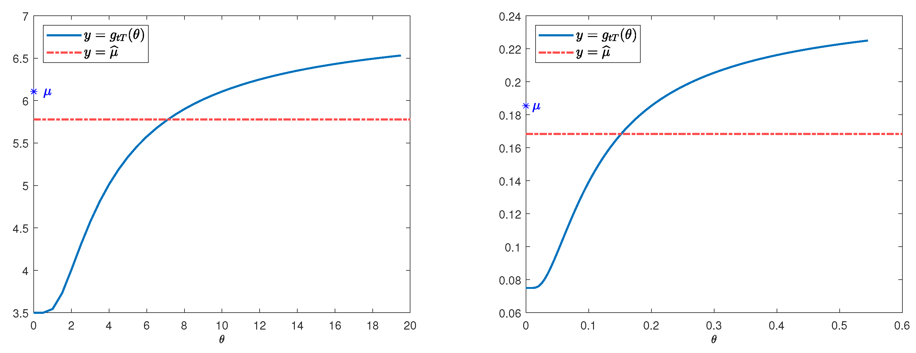
Due to the intense nature of the function , it is complicated to come up with an analytic justification establishing whether it is increasing or decreasing. But, at least for , appears to be an increasing function of as shown in Figure 1. Generally, we summarize the result in the following conjecture.
Conjecture 1.
The function is strictly increasing.
Proposition 2.
The function has the following limiting values
Proof.
These limits can be established by using L’Hôpital’s rule. □
Now, assuming the Conjecture 1 is true, then with Proposition 2, we have
Theorem 1.
The equation has a unique solution provided that
Solve the equation for , say . Then, again by the delta method, we conclude that . Note that if both the left- and right-truncation points lie on the same interval, then . So, the parameter to be estimated disappears from the equation, and hence we do not consider this case for further investigation. Define
Then, we obtain a fixed point function as , where
However, we need to consider the condition . Therefore, we need to be careful about the initialization of as the right truncation point T cannot be a boundary point because, if it was, then and we would not be able to divide by in the fixed point function .
Now, let us compute the derivative of with respect to using implicit differentiation.
- Case 1: Assume that the two truncation points are in two consecutive intervals, i.e., assume that . Then, , where
- Case 2: The other case is that the two truncation points are not in the two consecutive intervals, i.e., assume that . Then, , where and , and are defined above.
To obtain the exponential grouped MLE, consider Then, following Xue and Song (2002), we have , where .
Note that after finding the derivative, can be expressed as
The asymptotic performance of the MTuM estimator is measured through the asymptotic relative efficiency (ARE) in comparison to the grouped MLE. The ARE (see, e.g., Serfling 1980; van der Vaart 1998) is defined as
The primary justification for employing the MLE as a standard/benchmark for comparison lies in its optimal asymptotic behavior in terms of variance, though this comes with the typical proviso of being subject to “under certain regularity conditions”. Therefore, the desired ARE as given by Equation (11) is computed as
4. Simulation Study
This section augments the theoretical findings established in Section 3 with simulations. The primary objective is to determine the sample size required for the estimators to be unbiased (acknowledging that they are asymptotically unbiased), to validate the asymptotic normality, and to ensure that their finite sample relative efficiencies (REs) are converging towards the respective AREs. For calculating the RE, the MLE is utilized as the reference point. Consequently, the concept of asymptotic relative efficiency outlined in Equation (11) is adapted for finite sample analysis as follows:
The design of the simulation is detailed below, covering both the generation of data and the computation of various statistics as described:
- (i)
- The underlying ground-up distribution is assumed to be exponential with a mean parameter .
- (ii)
- Different sample sizes are explored: .
- (iii)
- A total of 1000 samples are generated for each scenario.
- (iv)
- The sample data are grouped according to the specified group boundaries: .
- (v)
- We consider the following vectors of group boundaries:
- (vi)
- For each grouping, 1000 estimates of are computed under the Method of Truncated Moments (MTuM) with varying truncation points for grouped data, denoted as .
- (vii)
- The average estimated , denoted , is calculated as .
- (vii)
- This process is repeated 10 times, yielding averages .
- (ix)
- The overall mean, , and the standard deviation, , of these averages are computed as follows:
- (x)
- (xi)
- Similarly, the finite-sample relative efficiency (RE) of the MTuM with respect to the grouped MLE is calculated as . The mean and standard deviations of these RE values are reported for different vectors of group boundaries.
The outcomes of the simulations are documented in Table 2, Table 3, Table 4, Table 5 and Table 6. The entries represent the ratios of the mean estimated values to the true parameter based on 1000 samples and repeated 10 times. That is, the ratio of the estimated and the true , as described in item x above. The corresponding standard errors are presented in parentheses. In all tables, the last three columns (with ∞) represent analytic results, not results from simulations. The third last column is for the asymptotic relative efficiency of the MTuM with regards to grouped MLE, coming from Equation (12) and Table 1. For example, the group boundary vectors considered in Table 1 and Table 4 are exactly the same and given by
Then, for , the corresponding entries in those two tables should match, and those matching entries, i.e., , are boxed in both tables. Similarly, the second last column is for the asymptotic relative efficiency of the MTuM with regards to un-grouped MLE, and the very last column represents the asymptotic relative efficiency of grouped MLE with regards to un-grouped MLE.
If both the truncation points are in the same interval, say , then we have . Therefore, the parameter to be estimated disappeared, and hence the four rows on Table 6 are reported as . As we move in sequence from Table 2, Table 3, Table 4, Table 5 and Table 6, it becomes noticeable that the convergence of the ratio of the estimated with the true , i.e., , approaches the true asymptotic value of 1 at a more gradual pace. This is because the length of intervals going from Table 2, Table 3, Table 4, Table 5 and Table 6 increases. More specifically, both our intuition and the data presented in the tables suggest that when there is a wider gap between the thresholds (namely, t and T), the estimators tend to approach the true values at a slower rate.
In Table 2, Table 3, Table 4 and Table 5, it is interesting to observe that, even for the sample size , the estimator successfully estimates their corresponding parameter , with less than of the relative bias, with one exception for . As seen in Table 6, the relative bias is within only for the sample of size and for . Similarly, as observed in those tables, it is clear that all the REs are asymptotically unbiased.
5. Concluding Remarks
In this scholarly work, we have introduced a novel Method of Truncated Moments (MTuM) estimator designed to estimate the tail index from grouped Pareto loss severity data, offering a robust alternative to maximum likelihood estimation (MLE). We have established theoretical justifications for the existence and asymptotic normality of the designed estimators. Additionally, we have conducted a detailed investigation into the finite sample performance across various sample sizes and group boundary vectors through a comprehensive simulation study.
Looking ahead, this paper predominantly addressed the estimation of the mean parameter of an exponential distribution (or equivalently, the tail index of a single-parameter Pareto distribution) using grouped sample data. Therefore, an avenue for future research is the extension of the proposed methodology to more complex scenarios and models. However, particularly for distributions with multiple parameters, examining the nature of the function , as presented in Equation (7) and Conjecture 1, can be highly challenging, if not infeasible. The task of providing asymptotic inferential justification for the MTuM methodology when applied to multi-parameter distributions presents similar difficulties. In this context, a potential direction for future research involves adopting an algorithmic approach (i.e., designing simulation-based estimators for complex models) rather than focusing solely on inferential justification, Efron and Hastie (2016, p. xvi).
Moreover, evaluating the performance of this novel MTuM estimator in diverse practical risk analysis scenarios remains an important area for further assessment. Attempting to apply the designed MTuM methodology to real grouped insurance data revealed the challenge of finding publicly available data that fit the single-parameter Pareto (or equivalently, an exponential) model well. This issue, along with the often poor fit of the data to the Pareto model, highlighted the importance of adapting the MTuM to many other distributions as well. Such adaptation will provide the necessary flexibility to select the most suitable underlying models based on the initial diagnostic tests of the datasets. Therefore, there is a need to broaden the theoretical development of the MTuM approach to at least include the location-scale family of distributions.
Funding
This research received no external funding.
Data Availability Statement
No new data were created or analyzed in this study. Data sharing is not applicable to this article.
Conflicts of Interest
The author declares no conflict of interest.
References
- Aigner, Dennis J., and Arthur S. Goldberger. 1970. Estimation of Pareto’s law from grouped observations. Journal of the American Statistical Association 65: 712–23. [Google Scholar] [CrossRef]
- Beran, Rudolf. 1977a. Minimum Hellinger distance estimates for parametric models. The Annals of Statistics 5: 445–63. [Google Scholar] [CrossRef]
- Beran, Rudolf. 1977b. Robust location estimates. The Annals of Statistics 5: 431–44. [Google Scholar] [CrossRef]
- Brazauskas, Vytaras, Bruce L. Jones, and Ričardas Zitikis. 2009. Robust fitting of claim severity distributions and the method of trimmed moments. Journal of Statistical Planning and Inference 139: 2028–43. [Google Scholar] [CrossRef]
- Chernoff, Herman, Joseph L. Gastwirth, and M. Vernon Johns. 1967. Asymptotic distribution of linear combinations of functions of order statistics with applications to estimation. Annals of Mathematical Statistics 38: 52–72. [Google Scholar] [CrossRef]
- Efron, Bradley, and Trevor Hastie. 2016. Computer Age Statistical Inference: Algorithms, Evidence, and Data Science. New York: Cambridge University Press. [Google Scholar] [CrossRef]
- Gatti, Selim, and Mario V. Wüthrich. 2023. Modeling lower-truncated and right-censored insurance claims with an extension of the MBBEFD class. arXiv arXiv:2310.11471. [Google Scholar]
- Kleiber, Christian, and Samuel Kotz. 2003. Statistical Size Distributions in Economics and Actuarial Sciences. Hoboken: John Wiley & Sons. [Google Scholar] [CrossRef]
- Klugman, Stuart A., Harry H. Panjer, and Gordon E. Willmot. 2019. Loss Models: From Data to Decisions, 5th ed. Hoboken: John Wiley & Sons. [Google Scholar]
- Lin, Nan, and Xuming He. 2006. Robust and efficient estimation under data grouping. Biometrika 93: 99–112. [Google Scholar] [CrossRef]
- Poudyal, Chudamani. 2021a. Robust estimation of loss models for lognormal insurance payment severity data. ASTIN Bulletin. The Journal of the International Actuarial Association 51: 475–507. [Google Scholar] [CrossRef]
- Poudyal, Chudamani. 2021b. Truncated, censored, and actuarial payment-type moments for robust fitting of a single-parameter Pareto distribution. Journal of Computational and Applied Mathematics 388: 113310. [Google Scholar] [CrossRef]
- Poudyal, Chudamani, Qian Zhao, and Vytaras Brazauskas. 2023. Method of winsorized moments for robust fitting of truncated and censored lognormal distributions. North American Actuarial Journal, 1–25. [Google Scholar] [CrossRef]
- Schader, Martin, and Friedrich Schmid. 1986. Optimal grouping of data from some skew distributions. Computational Statistics Quarterly 3: 151–59. [Google Scholar]
- Serfling, Robert J. 1980. Approximation Theorems of Mathematical Statistics. New York: John Wiley & Sons. [Google Scholar]
- Tukey, John W. 1960. A survey of sampling from contaminated distributions. In Contributions to Probability and Statistics. Stanford: Stanford University Press, pp. 448–85. [Google Scholar]
- van der Vaart, Aad W. 1998. Asymptotic Statistics. Cambridge: Cambridge University Press. [Google Scholar] [CrossRef]
- Victoria-Feser, Maria-Pia, and Elvezio Ronchetti. 1997. Robust estimation for grouped data. Journal of the American Statistical Association 92: 333–40. [Google Scholar] [CrossRef]
- Xue, Hongqi, and Lixin Song. 2002. Asymptotic properties of MLE for Weibull distribution with grouped data. Journal of Systems Science and Complexity 15: 176–86. [Google Scholar]
- Zhao, Qian, Vytaras Brazauskas, and Jugal Ghorai. 2018. Robust and efficient fitting of severity models and the method of Winsorized moments. ASTIN Bulletin 48: 275–309. [Google Scholar] [CrossRef]
Figure 1.
Graphs of for different values of . Left panel represents the graph of for , , and group boundaries vector . Similarly, right panel represents the graph of for , , and group boundaries vector .
Figure 1.
Graphs of for different values of . Left panel represents the graph of for , , and group boundaries vector . Similarly, right panel represents the graph of for , , and group boundaries vector .


Table 1.
Numerical values of given by Equation (12) for selected t and T with from . The truncation thresholds t and T are rounded to two decimal places, for example, , etc.
Table 1.
Numerical values of given by Equation (12) for selected t and T with from . The truncation thresholds t and T are rounded to two decimal places, for example, , etc.
| t(F(t)) | |||||||
|---|---|---|---|---|---|---|---|
| 70(0.001) | 45(0.01) | 35(0.03) | 25(0.08) | 19(0.15) | 12(0.30) | 7(0.50) | |
| 00.0(0.00) | 0.870 | 0.762 | 0.584 | 0.350 | 0.224 | 0.093 | 0.038 |
| 00.5(0.05) | 0.869 | 0.760 | 0.583 | 0.349 | 0.225 | 0.095 | 0.038 |
| 01.0(0.10) | 0.865 | 0.756 | 0.579 | 0.347 | 0.225 | 0.098 | 0.038 |
| 02.0(0.14) | 0.841 | 0.731 | 0.559 | 0.334 | 0.220 | 0.105 | 0.038 |
| 03.0(0.26) | 0.782 | 0.675 | 0.512 | 0.302 | 0.201 | 0.114 | 0.038 |
| 07.0(0.50) | 0.483 | 0.396 | 0.274 | 0.131 | 0.071 | 0.023 | – |
| 14.0(0.75) | 0.214 | 0.156 | 0.087 | 0.027 | 0.014 | – | – |
| 19.0(0.85) | 0.118 | 0.074 | 0.033 | 0.009 | – | – | – |
| 23.0(0.90) | 0.076 | 0.041 | 0.014 | – | – | – | – |
Note: The boxed entry will be compared with an entry from Table 4.
Table 2.
Finite-sample performance evaluation of MTuM with regards to MLE for grouped data from an exponential () and group boundaries vector .
Table 2.
Finite-sample performance evaluation of MTuM with regards to MLE for grouped data from an exponential () and group boundaries vector .
| MTuM Performance for Exponential Grouped Data | ||||||||||
|---|---|---|---|---|---|---|---|---|---|---|
| 50 | 100 | 250 | 500 | 1000 | ∞ | ∞ | ∞ | |||
| 0 | 200 | 1.00(0.003) | 1.00(0.003) | 1.00(0.002) | 1.00(0.001) | 1.00(0.001) | 1 | - | - | |
| 0 | 50 | 1.01(0.004) | 1.00(0.002) | 1.00(0.002) | 1.00(0.001) | 1.00(0.001) | 1 | - | - | |
| 0 | 100 | 1.00(0.003) | 1.00(0.003) | 1.00(0.001) | 1.00(0.001) | 1.00(0.001) | 1 | - | - | |
| 0 | 140 | 1.00(0.005) | 1.00(0.004) | 1.00(0.002) | 1.00(0.001) | 1.00(0.001) | 1 | - | - | |
| 2 | 12 | 3.22(0.174) | 1.68(0.130) | 1.14(0.021) | 1.06(0.012) | 1.03(0.005) | 1 | - | - | |
| RE | 0 | 200 | 1.01(0.032) | 1.02(0.037) | 1.02(0.039) | 0.99(0.045) | 0.99(0.048) | 1.00 | 1.00 | 1.00 |
| 0 | 50 | 0.77(0.048) | 0.79(0.058) | 0.81(0.032) | 0.84(0.035) | 0.83(0.028) | 0.82 | 0.82 | 1.00 | |
| 0 | 100 | 1.00(0.045) | 0.98(0.040) | 1.02(0.050) | 0.99(0.034) | 0.99(0.046) | 1.00 | 0.99 | 1.00 | |
| 0 | 140 | 0.96(0.042) | 1.01(0.063) | 0.97(0.047) | 1.00(0.047) | 1.01(0.033) | 1.00 | 1.00 | 1.00 | |
| 2 | 12 | 0.00(0.000) | 0.00(0.000) | 0.01(0.004) | 0.02(0.004) | 0.03(0.002) | 0.04 | 0.04 | 1.00 | |
Table 3.
Finite-sample performance evaluation of MTuM with regards to MLE for grouped data from an exponential () and group boundaries vector .
Table 3.
Finite-sample performance evaluation of MTuM with regards to MLE for grouped data from an exponential () and group boundaries vector .
| MTuM Performance for Exponential Grouped Data | ||||||||||
|---|---|---|---|---|---|---|---|---|---|---|
| 50 | 100 | 250 | 500 | 1000 | ∞ | ∞ | ∞ | |||
| 0 | 200 | 1.00(0.006) | 1.00(0.003) | 1.00(0.002) | 1.00(0.001) | 1.00(0.001) | 1 | - | - | |
| 0 | 50 | 1.01(0.005) | 1.00(0.003) | 1.00(0.002) | 1.00(0.002) | 1.00(0.001) | 1 | - | - | |
| 0 | 100 | 1.00(0.006) | 1.00(0.003) | 1.00(0.002) | 1.00(0.002) | 1.00(0.001) | 1 | - | - | |
| 0 | 140 | 1.00(0.005) | 1.00(0.004) | 1.00(0.002) | 1.00(0.001) | 1.00(0.001) | 1 | - | - | |
| 2 | 12 | 3.17(0.169) | 1.67(0.083) | 1.16(0.024) | 1.05(0.007) | 1.03(0.006) | 1 | - | - | |
| RE | 0 | 200 | 1.00(0.061) | 0.99(0.071) | 0.99(0.047) | 0.98(0.068) | 1.04(0.049) | 1.00 | 1.00 | 1.00 |
| 0 | 50 | 0.75(0.054) | 0.81(0.037) | 0.81(0.023) | 0.82(0.038) | 0.84(0.038) | 0.82 | 0.82 | 1.00 | |
| 0 | 100 | 0.99(0.047) | 0.96(0.039) | 0.99(0.065) | 1.03(0.043) | 0.99(0.057) | 1.00 | 0.99 | 1.00 | |
| 0 | 140 | 0.99(0.028) | 1.02(0.046) | 1.02(0.050) | 1.00(0.041) | 1.01(0.043) | 1.00 | 1.00 | 1.00 | |
| 2 | 12 | 0.00(0.000) | 0.00(0.000) | 0.01(0.003) | 0.02(0.004) | 0.03(0.001) | 0.04 | 0.04 | 1.00 | |
Table 4.
Finite-sample performance evaluation of MTuM with regards to MLE for grouped data from an exponential () and group boundaries vector .
Table 4.
Finite-sample performance evaluation of MTuM with regards to MLE for grouped data from an exponential () and group boundaries vector .
| MTuM Performance for Exponential Grouped Data | ||||||||||
|---|---|---|---|---|---|---|---|---|---|---|
| Sample Size, n | ||||||||||
| 50 | 100 | 250 | 500 | 1000 | ∞ | ∞ | ∞ | |||
| 0 | 200 | 1.00(0.004) | 1.00(0.003) | 1.00(0.002) | 1.00(0.002) | 1.00(0.001) | 1 | - | - | |
| 0 | 50 | 1.01(0.005) | 1.00(0.003) | 1.00(0.002) | 1.00(0.001) | 1.00(0.001) | 1 | - | - | |
| 0 | 100 | 1.00(0.004) | 1.00(0.003) | 1.00(0.002) | 1.00(0.001) | 1.00(0.001) | 1 | - | - | |
| 0 | 140 | 1.00(0.004) | 1.00(0.004) | 1.00(0.003) | 1.00(0.002) | 1.00(0.001) | 1 | - | - | |
| 2 | 12 | 1.41(0.062) | 1.13(0.019) | 1.04(0.007) | 1.02(0.003) | 1.01(0.004) | 1 | - | - | |
| RE | 0 | 200 | 0.88(0.026) | 0.91(0.049) | 0.88(0.027) | 0.87(0.033) | 0.86(0.037) | 0.86 | 0.84 | 0.97 |
| 0 | 50 | 0.79(0.043) | 0.79(0.044) | 0.81(0.045) | 0.82(0.019) | 0.82(0.028) | 0.83 | 0.80 | 0.97 | |
| 0 | 100 | 0.92(0.036) | 0.94(0.030) | 0.94(0.033) | 0.94(0.038) | 0.94(0.031) | 0.95 | 0.92 | 0.97 | |
| 0 | 140 | 1.01(0.078) | 0.99(0.047) | 1.01(0.040) | 0.94(0.038) | 1.02(0.038) | 1.00 | 0.97 | 0.97 | |
| 2 | 12 | 0.01(0.002) | 0.03(0.007) | 0.07(0.005) | 0.09(0.004) | 0.10(0.006) | 0.11 | 0.10 | 0.97 | |
Note: The boxed entry is identical to the boxed entry from Table 1.
Table 5.
Finite-sample performance evaluation of MTuM with regards to MLE for grouped data from an exponential () and group boundaries vector .
Table 5.
Finite-sample performance evaluation of MTuM with regards to MLE for grouped data from an exponential () and group boundaries vector .
| MTuM Performance for Exponential Grouped Data | ||||||||||
|---|---|---|---|---|---|---|---|---|---|---|
| n | ||||||||||
| 50 | 100 | 250 | 500 | 1000 | ∞ | ∞ | ∞ | |||
| 0 | 200 | 1.00(0.002) | 1.00(0.004) | 1.00(0.002) | 1.00(0.001) | 1.00(0.001) | 1 | - | - | |
| 0 | 50 | 1.01(0.007) | 1.00(0.004) | 1.00(0.002) | 1.00(0.001) | 1.00(0.001) | 1 | - | - | |
| 0 | 100 | 1.00(0.006) | 1.00(0.003) | 1.00(0.002) | 1.00(0.002) | 1.00(0.001) | 1 | - | - | |
| 0 | 140 | 1.00(0.006) | 1.00(0.002) | 1.00(0.002) | 1.00(0.001) | 1.00(0.001) | 1 | - | - | |
| 2 | 12 | 1.16(0.022) | 1.06(0.007) | 1.02(0.005) | 1.01(0.004) | 1.01(0.002) | 1 | - | - | |
| RE | 0 | 200 | 1.00(0.032) | 1.03(0.038) | 1.00(0.036) | 0.99(0.049) | 1.01(0.048) | 1.00 | 0.92 | 0.92 |
| 0 | 50 | 0.76(0.054) | 0.78(0.031) | 0.78(0.028) | 0.80(0.031) | 0.81(0.027) | 0.81 | 0.74 | 0.92 | |
| 0 | 100 | 0.97(0.064) | 0.97(0.038) | 1.00(0.034) | 0.97(0.053) | 0.99(0.026) | 1.00 | 0.92 | 0.92 | |
| 0 | 140 | 0.99(0.042) | 1.00(0.061) | 1.01(0.058) | 1.00(0.024) | 1.01(0.044) | 1.00 | 0.92 | 0.92 | |
| 2 | 12 | 0.04(0.010) | 0.11(0.020) | 0.16(0.010) | 0.18(0.007) | 0.18(0.008) | 0.18 | 0.17 | 0.92 | |
Table 6.
Finite-sample performance evaluation of MTuM with regards to MLE for grouped data from an exponential () and group boundaries vector .
Table 6.
Finite-sample performance evaluation of MTuM with regards to MLE for grouped data from an exponential () and group boundaries vector .
| MTuM Performance for Exponential Grouped Data | ||||||||||
|---|---|---|---|---|---|---|---|---|---|---|
| n | ||||||||||
| 50 | 100 | 250 | 500 | 1000 | ∞ | ∞ | ∞ | |||
| MEAN | 0 | 200 | 0.68(0.011) | 0.78(0.007) | 0.91(0.006) | 0.97(0.003) | 0.99(0.002) | 1 | - | - |
| 0 | 50 | n/a | n/a | n/a | n/a | n/a | n/a | - | - | |
| 0 | 100 | 0.68(0.011) | 0.78(0.008) | 0.91(0.011) | 0.97(0.004) | 0.99(0.003) | 1 | - | - | |
| 0 | 140 | 0.68(0.011) | 0.78(0.014) | 0.92(0.006) | 0.97(0.004) | 0.99(0.002) | 1 | - | - | |
| 2 | 12 | n/a | n/a | n/a | n/a | n/a | n/a | - | - | |
| RE | 0 | 200 | 0.43(0.003) | 0.31(0.006) | 0.32(0.014) | 0.52(0.033) | 0.84(0.079) | 1.00 | 0.17 | 0.17 |
| 0 | 50 | n/a | n/a | n/a | n/a | n/a | n/a | - | - | |
| 0 | 100 | 0.43(0.007) | 0.30(0.007) | 0.32(0.018) | 0.53(0.060) | 0.84(0.046) | 0.97 | 0.17 | 0.17 | |
| 0 | 140 | 0.43(0.006) | 0.31(0.009) | 0.34(0.018) | 0.55(0.030) | 0.87(0.058) | 1.00 | 0.17 | 0.17 | |
| 2 | 12 | n/a | n/a | n/a | n/a | n/a | n/a | - | - | |
Disclaimer/Publisher’s Note: The statements, opinions and data contained in all publications are solely those of the individual author(s) and contributor(s) and not of MDPI and/or the editor(s). MDPI and/or the editor(s) disclaim responsibility for any injury to people or property resulting from any ideas, methods, instructions or products referred to in the content. |
© 2024 by the author. Licensee MDPI, Basel, Switzerland. This article is an open access article distributed under the terms and conditions of the Creative Commons Attribution (CC BY) license (https://creativecommons.org/licenses/by/4.0/).
Share and Cite
MDPI and ACS Style
Poudyal, C. Robust Estimation of the Tail Index of a Single Parameter Pareto Distribution from Grouped Data. Risks 2024, 12, 45. https://doi.org/10.3390/risks12030045
AMA Style
Poudyal C. Robust Estimation of the Tail Index of a Single Parameter Pareto Distribution from Grouped Data. Risks. 2024; 12(3):45. https://doi.org/10.3390/risks12030045
Chicago/Turabian StylePoudyal, Chudamani. 2024. "Robust Estimation of the Tail Index of a Single Parameter Pareto Distribution from Grouped Data" Risks 12, no. 3: 45. https://doi.org/10.3390/risks12030045
Note that from the first issue of 2016, this journal uses article numbers instead of page numbers. See further details here.