Market Equilibrium and the Cost of Capital with Heterogeneous Investment Horizons

Abstract

Expected returns, variances, betas, and alphas are all non-linear functions of the investment horizon. This seems to be a fatal conceptual problem for the capital asset pricing model (CAPM), which assumes a unique common horizon for all investors. We show that under the standard assumptions, the theoretical CAPM equilibrium surprisingly holds with the 1-period parameters, even when investors have heterogeneous and possibly much longer horizons. This is true not only for risk-averse investors, but for any investors with non-decreasing preferences, including prospect theory investors. Thus, the widespread practice of using monthly betas to estimate the cost of capital is theoretically justified.

1. Introduction

A young person saving for retirement has a planned investment horizon of several decades. The horizon of a person in her eighties is obviously much shorter. How should this dramatic difference influence the composition of their equity portfolios? Should fund managers consider the typical horizon of their clientele when determining how much to invest in each stock? Betas systematically depend on the horizon—should estimates of the cost of capital be based on betas corresponding to investors’ average or ‘typical’ horizon? From a macro perspective, what are the effects on the market equilibrium of lengthening this horizon due to increased life expectancy? This is a crucial issue, in light of the fact that life expectancy has increased steadily and substantially over the last century, from about 47 years in 1900 to 78 years today, that is, by about 3 months per year (Cutler et al. 2006). If this trend continues, what will be the asset pricing implications?

This paper examines the implications of the investment horizon, and in particular, the heterogeneity of horizons, on the risk–return equilibrium, and the cost of capital. In practice, the main method for estimating the cost of capital is to employ the CAPM risk–return relationship with monthly betas. While the debate about the empirical validity of the CAPM has been ongoing for decades,1 there is no question about the central role of the CAPM as a conceptual cornerstone, and as an extremely valuable practical tool for capital budgeting. The vast majority of managers employ the CAPM risk–return relationship with monthly parameters to estimate the cost of capital (Graham and Harvey 2001; Jacobs and Shivdasani 2012; Mukhlynina and Nyborg 2016; and Berk and van Binsbergen 2017).2 Are all these managers making a fundamental mistake when they employ monthly CAPM betas to estimate the cost of capital? After all, investors’ horizons are typically much longer than one month, and it is well known that betas change systematically and significantly with the investment horizon.

This research does not contribute to the empirical debate about the validity of the CAPM. Rather, our main contribution is a theoretical one. We show that one of the model’s central unrealistic assumptions, that of a homogeneous investment horizon, can be relaxed. If the 1-period (e.g., monthly) returns are normal and serially independent, the CAPM theoretically holds with the 1-period parameters, even if investors have heterogeneous horizons much longer than 1 period, and they are not necessarily risk-averse. Thus, the widespread practice of employing monthly betas to estimate the cost of capital is perfectly justified from a theoretical standpoint.

This result may seem surprising, given the non-linear dependence of the return parameters on the horizon. Even more problematic is the fact that as the horizon lengthens, the return distributions become positively skewed, and therefore the mean–variance framework becomes inappropriate altogether, as discussed in the next section. We circumvent these problems by employing the stochastic dominance framework, which applies to any return distributions. We employ first-degree stochastic dominance (FSD); therefore, our equilibrium result holds not only for risk averters, but for any investors with non-decreasing utility (or value) functions.

There is a widespread perception of the CAPM as either a 1-period model, or alternatively a continuous-time model that requires continuous trading, both of which are unrealistic. We suggest that this perception should be re-evaluated—the model holds in discrete time with heterogeneous and even ambiguous investment horizons. Market equilibrium is invariant to the distribution of horizons across investors, and should not be affected by the increase in life expectancy. Fund managers should not be concerned with their investors’ horizons—their sole goal should be to maximize the fund’s 1-period Sharpe ratio.

The next section reviews the related literature. Our main theoretical results are presented in Section 3. Section 4 examines the robustness of the theoretical results to relaxing the assumptions of normality and serial independence. Section 5 concludes with a discussion of the implications.

2. Related Literature

The investment horizon, and in particular, market equilibrium under heterogeneous horizons, are central challenges of financial economics (Levy 2022). Two key issues related to the investment horizon are (a) the optimal asset allocation between stocks and the risk-free asset, and (b) the optimal diversification across stocks and the implications for asset pricing and the cost of capital. While the first issue has been extensively discussed, the second, which is the focus of the present study, has attracted much less attention. Horizon effects are complex because expected returns, variances, correlations, betas, and alphas are all non-linear functions of the horizon (Tobin 1958; Levhari and Levy 1977; Bessembinder et al. 2021, 2023). Betas change systematically and non-linearly with the horizon: under i.i.d. returns, the betas of defensive stocks decrease with the horizon, while the betas of aggressive stocks increase with the horizon (Levhari and Levy 1977; Handa et al. 1989; and Bessembinder et al. 2021). As a consequence, a stock may have a positive alpha when calculated with 1-period returns, but a negative alpha when T-period returns are employed, or vice versa. In general, an investor’s optimal stock mix depends on her investment horizon, and therefore equilibrium asset prices and the risk–return relationship seem to depend on the distribution of horizons across investors.

Since the heterogeneity of investment horizons is a central property of the capital market, and given that we have yet to find a clearly superior alternative to the CAPM, several researchers have made advances in generalizing the CAPM to settings with heterogeneous horizons. The main approach taken in this literature is to assume that investors have mean–variance preferences, where the portfolio mean and variance considered correspond to the investor’s horizon. Lee et al. (1990) derived market equilibrium under heterogeneous investment horizons in this setting. Martellini and Urošević (2006) analyzed the case of investors with mean–variance preferences and a stochastic investment horizon. Brennan and Zhang (2020) developed an asset pricing model where investors have homogeneous mean–variance preferences and their investment horizons are stochastically drawn from the same distribution. Moreover, they showed that their model empirically outperforms both the standard CAPM and the Fama and French (1993) 3-factor model.

Mean–variance preferences are consistent with expected utility maximization in the following four cases: (i) the return distributions are normal (or, more generally, elliptical); (ii) the utility function is quadratic; (iii) returns are small in absolute value (Levy and Markowitz 1979); and (iv) under a continuous-time return generating process with continuous portfolio rebalancing (Merton 1971, 1973, 1990). Unfortunately, none of these conditions hold in a realistic setting with long investment horizons. Even if the 1-period return distributions are normal, the T-period return distributions are not; as the investment horizon increases, positive skewness builds up (Arditti and Levy 1975; Bessembinder 2018), and the return distributions diverge from normality. Quadratic preference implies the unrealistic property of increasing absolute risk aversion (Arrow 1971), while monthly returns are relatively small in absolute magnitude. This is no longer true for annual returns, let alone returns calculated over several years. In this case, mean–variance optimization no longer provides a good approximation for direct expected utility maximization, as shown by Levy and Markowitz (1979). Finally, continuous trading breaks down under even the slightest trading costs and, in addition, the standard continuous model implies that the return distribution over any finite horizon is lognormal, which is inconsistent with the empirical evidence (Levy and Duchin 2004). Thus, when the horizons are long, it is difficult to justify mean–variance preferences.

This motivates us to adopt a different approach that does not rely on mean–variance preferences over long horizons. Rather, we employ the distribution-free stochastic dominance approach. This framework does not make any assumptions about the shape of the T-period return distributions, and the only assumption about preferences is that investors’ utility functions are non-decreasing (we employ first-degree stochastic dominance). Thus, the results apply not only to all risk averters, but also to investors with prospect theory preferences (Kahneman and Tversky 1979; Tversky and Kahneman 1992) and investors with various aspiration levels (Payne et al. 1980; Payne 2005).

3. Theoretical Results

We begin by proving that the standard discrete-time CAPM holds under heterogeneous investment horizons for all investors with any non-decreasing preferences. Then, we extend the results to the case where a risk-free asset does not exist (i.e., Black’s (1972) zero-beta version), to the case where return parameters vary over time (i.e., the conditional version of the model), and to the case where investors have labor income and utility defined over both intermediate and terminal consumption.

• Preliminaries

(1)

First-degree Stochastic Dominance (FSD)

Let F and G denote the cumulative distribution functions of the returns of two alternative investment prospects, F and G. Then, investment F is preferred over investment G by all investors with non-decreasing utility (or value) functions if and only if $F\left(x\right)\le G\left(x\right)$ for all values x, and a strict inequality holds for at least one value $x_0$ (see Hadar and Russell 1969; Hanoch and Levy 1969). Note that FSD implies preference not only by all expected utility maximizers, but also by cumulative prospect theory investors, possibly employing probability weighting (Tversky and Kahneman 1992).

(2)

FSD among Investments with Normal Returns

In the special case where the returns on investments F and G are normally distributed with means ${\mu }_F and {\mu }_G$ and standard deviations ${\sigma }_F and {\sigma }_G$, respectively, the condition for FSD dominance of F over G becomes the following: ${\mu }_F>{\mu }_G$ and ${\sigma }_F={\sigma }_G$ (Hanoch and Levy 1969, p. 343).

(3)

Multi-Period FSD

Consider two alternative multi-period investment strategies, F and G:

F: investing in portfolio $F_1$ in period 1, in $F_2$ in period 2, … and in $F_T$ in period T.

G: investing in portfolio $G_1$ in period 1, in $G_2$ in period 2, … and in $G_T$ in period T.

The total returns (i.e., 1+ rates of return) are multiplicative: the total return after T periods is $R_1{R}_2\dots R_T$, where $R_t$ is the total return in period t. Under the assumption that the returns are independent over time (but not necessarily identically distributed), the following holds: if portfolio $F_1$ FSD dominates portfolio $G_1$, portfolio $F_2$ FSD dominates portfolio $G_2$, etc., then the multi-period investment strategy F FSD dominates investment strategy G (Levy 1973, Theorem 2).

The above results are employed below to derive equilibrium under heterogeneous horizons. Consider a market with N risky assets and a risk-free asset. As opposed to the standard CAPM, investors may have heterogeneous investment horizons, and we denote investor i’s horizon by $T_i$. We begin by assuming that $T_i$ is deterministic, and later extend the results to the case where the horizon is stochastic, or even ambiguous. Investor i maximizes her expected utility defined over terminal wealth at horizon $T_i$. Investors may revise their portfolios every period. Denote the portfolio weight of investor i in asset j at period t by $x_{j,t}^i$, and the weight in the risk-free asset by $x_{r_f,t}^i$, implying a period-t portfolio return of the following:

$${\tilde{R}}_{pt}^i={\sum }_{j=1}^N{x}_{j,t}^i{\tilde{R}}_j+x_{r_f,t}^i{r}_f,$$

(1)

where ${\tilde{R}}_j$ denotes the stochastic return (1 + rate of return) of asset j, and $r_f$ is the return on the risk-free asset. Given a strategy of holding portfolio weights $x_{j,t}^i$ in period t, investor i’s terminal wealth after $T_i$ investment periods is given by the following:

$${\tilde{W}}_{T_i}^i=W_0^i{\tilde{R}}_{p1}^i{\tilde{R}}_{p2}^i\dots {\tilde{R}}_{p{T}_i}^i,$$

(2)

where $W_0^i$ denotes investor i’s initial wealth, and the portfolio returns are given by (1). The investor maximizes the expected utility defined over her terminal wealth as follows:

$$EU=E\left[U^i\left({\tilde{W}}_{T_i}^i\right)\right],$$

(3)

where $U^i$ denotes investor i’s utility function.

In the case of constant relative risk aversion (CRRA) utility and i.i.d returns, the solution to the EU maximization problem (3) is independent of the investment horizon. However, this is not generally true for other utility functions. In general, the optimal strategy $x_{j,t}^i$ may depend not only on the investor’s utility function, but also on the initial wealth $W_0^i$ and on the investment horizon $T_i$.

We consider a framework where investors need not necessarily be risk-averse: they may have any non-decreasing utility functions, including functions with risk-seeking segments and various aspiration levels. Investors may also be prospect theory expected value maximizers with a value function defined over the difference between the terminal wealth and some reference point and subjective CPT decision weights.

Theorem 1. 

Under the standard CAPM assumptions of homogeneous expectations and the normality of 1-period return distributions, and the additional assumption that returns are independent over time, the CAPM equilibrium holds, with the 1-period return parameters.

Proof. 

Consider an investor with a horizon of T periods, employing a strategy G of investing in portfolio $G_1$ in period 1, in portfolio $G_2$ in period 2, etc., as illustrated by Figure 1. Consider an alternative strategy F, with portfolio $F_1$ vertically above $G_1$, in period 1, $F_2$ vertically above $G_2$ in period 2, etc., as illustrated in the figure. Notice that strategy F is based on portfolios that are mixtures of the 1-period equity tangency portfolio T and the risk-free asset. As the 1-period return distributions are, by assumption, normal, and ${\mu }_{F_t}>{\mu }_{G_t}$ and ${\sigma }_{F_t}={\sigma }_{G_t}$ for all periods t, by preliminary result (2) $F_t$ FSD dominates $G_t$. Preliminary result (3) implies that strategy F FSD dominates strategy G.3 This dominance is invariant to the investor’s initial wealth. Thus, the optimal equity portfolio for all investors, regardless of their horizon, their utility function, and their initial wealth, should be the 1-period tangency portfolio. Note that as the dominance is by FSD, this is true not only for risk-averse investors, but for all investors with non-decreasing utility functions, including investors with prospect theory preferences.4 By market clearance, the market portfolio must coincide with the tangency portfolio.5 Following the standard analysis, the mean–variance efficiency of the market portfolio implies the CAPM linear risk–return relationship (Merton 1972; Roll 1977). Q.E.D. □

It is important to note that while investors’ horizons may be long, the CAPM holds with the 1-period parameters. In other words, the market portfolio coincides with the tangency portfolio that is derived with the 1-period return parameters, and the linear risk–return relationship holds between the 1-period expected returns and the 1-period betas. As Levhari and Levy (1977) and Bessembinder et al. (2021) show, the model will not hold when return parameters are calculated with longer horizons.

• Extensions

Theorem 1 can be extended to the case of stochastic or ambiguous horizons, the case where a risk-free asset does not exist, the case where parameters vary over time, and the case where investors earn labor income and utility defined over both intermediate and terminal consumption.

(i)

Stochastic or Ambiguous Investment Horizons

Theorem 1 shows that the investor’s optimal equity portfolio is the 1-period mean–variance tangency portfolio, regardless of the investor’s horizon. As this result holds for any horizon, it obviously also holds if the horizon is stochastic, or even if it is ambiguous, i.e., if the horizon is drawn from an unknown distribution.

(ii)

No Risk-Free Asset

A very similar analysis can be conducted when a risk-free asset does not exist, following Black (1972). Consider a strategy G, which implies investing in portfolio $G_1$ in period 1, in $G_2$ in period 2, … and in $G_T$ in period T. Compare this strategy with strategy F^*, which implies holding portfolios $F_1^{*},F_2^{*},\dots ,F_T^{*}$, which are located on the 1-period mean–variance efficient frontier, directly above the corresponding portfolios $G_1,G_2,\dots ,G_T$, as shown in Figure 2. Following the analysis of Theorem 1, strategy F^* dominates strategy G by FSD. This implies that all investors with non-decreasing preferences should always choose their portfolios on the 1-period mean–variance efficient frontier. The market portfolio is a wealth-weighted average of all individual investors’ portfolios, and as these are on the efficient frontier, so is the market portfolio (Black 1972). It follows that the CAPM linear risk–return relationship holds for the 1-period parameters with the zero-beta rate replacing the risk-free rate, exactly as in Black’s analysis.

(iii)

Time-Varying Return Parameters

In Figure 1 and Figure 2, the same 1-period mean–variance frontier is drawn for all periods, which may seem to imply that the return parameters are assumed to be constant over time. However, this need not be the case. The parameters may be time-varying. At every period, investors derive the 1-period mean–variance frontier and the tangency portfolio based on the return parameters conditional on all information at that time. When new information arrives to the market, the parameters may change, and therefore so may the frontier and the tangency portfolio. Thus, the market portfolio may be time-varying. However, at any point in time, the market portfolio is the mean–variance optimal equity portfolio for the next period, and the CAPM risk–return relationship holds with the 1-period new ex ante parameters, based on the information available at that time. Thus, the results extend to the case of time-varying returns and possible regime switches (Ang and Bekaert 2002).

(iv)

Intermediate Income and Consumption

The standard CAPM, as well as its generalization in Theorem 1, assume that the investor’s utility (or value) is defined over terminal wealth. In a multiple-period setting, intermediate income and consumption are likely to also be important, especially when the investor’s horizon is long. The result of Theorem 1 can be extended to the case of intermediate income and consumption, as proven in the Supplementary Materials Section S1.

4. Relaxing the Assumptions of 1-Period Normality and Serial Independence

The theoretical results in the preceding section rely on three main assumptions: (i) homogeneous expectations (ii) normality of the 1-period return distributions, and (iii) serial independence of the returns. The extension of the CAPM to the case of heterogeneous expectations has been discussed by several studies, including Lintner (1969), Williams (1977), DeMarzo and Skiadas (1998), Barberis et al. (2015), and Shi (2016). Therefore, in this study we focused on the effects of relaxing assumptions (ii) and (iii).

If the 1-period returns are normally distributed and are independent over time, Theorem 1 proves that all investors, regardless of their investment horizon and preference, will optimally hold mixtures of the 1-period mean–variance tangency portfolio and the risk-free asset. In practice, the 1-period return distributions may deviate from normality and may be serially correlated. To examine the validity of the theoretical results under realistic return distributions and serial correlations, we employed the empirical monthly return distributions as the ex ante 1-period return distributions. This should not be taken to imply that we believe that the ex post distributions are the best estimates of the ex ante distributions. Rather, we simply employ the empirical distributions to reflect “typical” return distributions, and, in particular, deviations from normality and serial-independence. We should stress that even though we employed the empirical returns, the following analysis is not an empirical test of the CAPM. Rather, it is a test of the robustness of our theoretical results to relaxation of the underlying assumptions. The choice of the “period” to be one month is in line with most empirical studies. One month is short enough so that the return distributions are pretty close to normal, yet not too short in the sense of implying very frequent portfolio revisions.

As a result of the deviations from normality and from serial independence, each investor may have a different optimal equity portfolio, depending on her horizon and utility function. For each investor, we numerically find the optimal portfolio that maximizes her expected utility, based on the terminal wealth distribution. Once we have each investors’ optimal equity portfolio, we calculate the aggregate market portfolio across all investors, and we evaluate the equilibrium relation between betas (with respect to this market portfolio) and expected returns.

4.1. Methodology and Data

Each investor maximizes her expected utility (or value) given by Equation (3). This maximization procedure is conducted numerically for each investor, where investors are heterogeneous across their horizons, T, and their preferences, U. For each investor, the horizon T is randomly drawn from a uniform distribution over the range of 1 year–20 years. We considered three classes of preferences, which are widely employed in the literature:

(1)

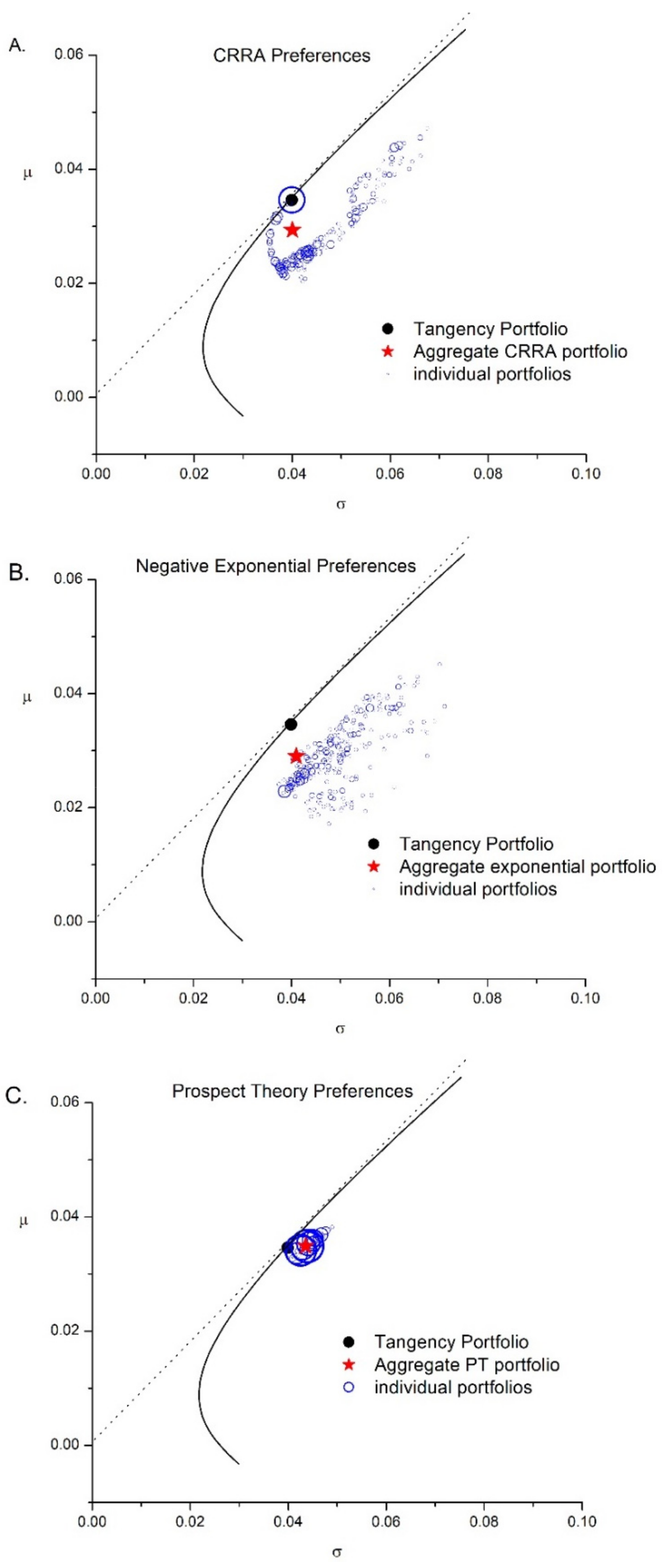
Constant relative risk aversion (CRRA): $U\left(W\right)=\frac{W^{1-\gamma }}{1-\gamma }$;

(2)

Negative exponential preferences (or CARA): $U\left(W\right)=-e^{-bW}$; and

(3)

Prospect theory preferences, given by the following:

$$V\left(x\right)=\left\{\begin{array}{c}{x}^{\alpha } for x>0\\ -\lambda {\left(-x\right)}^{\beta } for x<0\end{array}\right.,$$

(4)

where x denotes the change in wealth, rather than terminal wealth, i.e., ${x=W_T-W}_0$ (Tversky and Kahneman 1992).

We simulated a market with 1000 investors, and took an (almost) equal number of investors from each of the above three preference classes (334 CRRA investors, 333 exponential investors, and 333 prospect theory investors). We employed typical preference parameters reported in the literature. For each CRRA investor, the relative risk aversion parameter, $\gamma$, was randomly drawn from a uniform distribution in the range [0.5–5].6 For each exponential investor, the parameter b was randomly drawn from a uniform distribution in the range [0–0.0001].7 For PT investors, we took $\alpha =\beta =0.88$, as in Tversky and Kahneman (1992), and the loss aversion parameter, $\lambda$, was taken as randomly drawn from a uniform distribution in the range [2–3].8 All investors were assumed to have the same initial wealth of $100,000.9

We employed the empirical monthly returns in the period April 2002–March 2022 (240 months), as reported by CRSP. We took the 100 largest firms (CRSP sharecode = 11), by April 2002 market values, that had complete return records over the sample period.10 The terminal wealth distribution could be generated either with the assumption of serial independence, or alternatively, with the empirical serial correlations. To examine the effects of serial correlations, we employed both approaches and compared the results. Let us elaborate.

Suppose that the investment horizon is T = 120 months. We draw 120 months (with replacement) at random from the empirical return distribution and calculate the terminal wealth $W_T$ by Equation (1). To obtain the entire distribution of ${\tilde{W}}_T$, we draw 100,000 such “histories” of 120 returns. This procedure assumes independence of the returns over time. To capture possible serial correlation effects, we do not draw each month independently as described above, but instead, we make 10 random draws of 12 consecutive months. (In general, if the investment horizon is M years, we make M draws of 12 consecutive months). As before, this is repeated 100,000 times to obtain the distribution of ${\tilde{W}}_T$. This procedure, which captures the empirical serial correlations, is the one we employed in this study. To isolate the effects of serial correlations, in the Supplementary Materials Section S3, we report the (very similar) results obtained under the assumption of serial independence. The monthly risk-free rate was taken as the average Fama–French risk-free rate in our sample period, which is 0.095%. The solution to each investor’s expected utility maximization problem was obtained numerically by employing Matlab’s fmincon function.

4.2. Results

The top panel of Figure 3 shows the mean–variance efficient frontier and tangency portfolio denoted by T (bold circle), based on the empirical 1-month returns. The optimal equity portfolio of each investor depends on her investment horizon and her preference, as explained above. Even though for most investors the horizon is much longer than one month, we can describe the investor’s optimal portfolio by its 1-month parameters, i.e., as a point in the 1-month mean–variance frontier.

Under the conditions of Theorem 1, we would expect all equity portfolios to coincide with the 1-period tangency portfolio. However, as the empirical return distributions are not precisely normal and returns may be serially correlated, optimal portfolios may be different than the tangency portfolio, as evident in the figure. Note that more than one investor may choose the same portfolio. To convey this information, the size of each circle represents the number of investors holding the portfolio. The figure also shows the market portfolio, which is the weighted average equity portfolio aggregated across all investors, and is depicted in the figure by a star. Thus, we distinguish between the tangency portfolio that is optimal under the assumptions of Theorem 1, and the market portfolio obtained numerically with empirical return distributions and serial correlations.

Panel A of Figure 3 reveals that some investors hold the tangency portfolio, as predicted by Theorem 1. However, many investors deviate from this portfolio, due to the non-normality and the serial correlation of the returns. While some portfolios deviate considerably from the tangency portfolio, most are rather close to it. Below, we analyze the deviations by preference and by investment horizon. The most important observation is that the deviations from the tangency portfolio do not seem to be systematic, and to a large extent, they cancel out. This is evident from the observation that the market portfolio, which is the aggregate portfolio across all investors, is rather close to the tangency portfolio.

As we have the market portfolio and the 1-month return distribution for each of the stocks, we can calculate the monthly return distribution of the market portfolio and the beta of each stock. The bottom panel of Figure 3 shows the relationship between betas and expected returns for all stocks in our sample. The figure shows that even though the return distributions deviate from normality and returns may be serially correlated, a large part of the cross-sectional variation in expected returns is explained by betas, with an R² of 89%. Thus, employing monthly betas provides a very good estimate of the cost of equity. We should emphasize again that this is not an empirical test of the CAPM—it only shows that realistic deviations from normality and serial independence do not have a very large impact on the theoretical results of Theorem 1.

It is interesting to note that most of the deviations from the theoretical predictions are due to deviations from normality, rather than to the serial correlations, which are relatively small. When we repeated the analysis by drawing each month independently (rather than a draw of 12 consecutive months), we obtained very similar results, as shown in Supplementary Materials Section S3. This is not surprising, given that the serial correlations are small: the average serial correlations of returns in our sample for lags of 1, 3, 6, and 12 months are −0.016, 0.005, −0.048, and −0.002, respectively.

Do the deviations from the tangency portfolio depend systematically on the preference class? Figure 4 shows investors’ equity portfolios by preference class, as well as the aggregate portfolio for each class. In all cases, there are deviations of the individual portfolios from the tangency portfolio, but these tend to cancel out, and the aggregate portfolio of all investors in a given preference class (depicted by a star) is rather close to the tangency portfolio. It is interesting to note that prospect theory preferences yield the smallest deviations from the tangency portfolio.

Figure 5 shows the results by the length of the horizon. We somewhat arbitrarily categorized horizons as short (1–5 years, Panel A), intermediate (6–10 years, Panel B), and long (11–20 years, Panel C). The star denotes the aggregate portfolio of all investors in each horizon category. For each category, we find that the aggregate portfolio is close to the tangency portfolio. In fact, the aggregate portfolios are even closer to the tangency portfolio compared with the case of aggregation across preference class (Figure 4). This may suggest that portfolio deviations among investors with similar horizons but different preference classes (Figure 5) tend to cancel each other more effectively than deviations among investors with the same preference class but different investment horizons (Figure 4).

It is well known that mean–variance portfolio optimization based on the sample return parameters leads to a tangency portfolio with many short positions (see, for example, Brennan and Lo 2010, and references therein). Stating that the market portfolio coincides with the tangency portfolio seems problematic for CAPM equilibrium, because the market portfolio by definition has only positive weights. However, Levy and Roll (2010) show that slight adjustments to the sample parameters, well within their estimation error confidence intervals, can lead to a tangency portfolio with weights that are identical to the weights of the market proxy. Our results are robust to employing the Levy–Roll adjustment to the sample parameters, leading to results that are very similar to those reported above (see Supplementary Materials Section S4).

5. Concluding Remarks

Almost six decades after its inception, the CAPM remains a cornerstone of financial economics. One of its two main predictions, that it is difficult to outperform the market index in terms of risk-adjusted returns, seems to have wide consensus.11 There is much less agreement about the model’s risk–return predictions. The empirical examination of this risk–return relationship is inherently difficult, primarily due to the large estimation error involved in the estimation of expected returns. However, it seems that we do not yet have a clearly superior alternative to the CAPM’s risk–return relationship. Indeed, most managers employ monthly CAPM betas to estimate the cost of capital (Graham and Harvey 2001; Jacobs and Shivdasani 2012; Mukhlynina and Nyborg 2016; Berk and van Binsbergen 2017).

Many academics view the CAPM as an important pedagogical tool, but one that has severe theoretical limitations. Namely, the model is typically perceived as being either a 1-period model, which cannot encompass the realistic complexities of heterogeneous investment horizons, or alternatively as a continuous-time model, which requires continuous trading that breaks down under even the smallest trading costs. Our findings suggest that this critical perception should be re-evaluated.

We show that under the standard assumptions of normality and homogeneous expectations, plus the assumption that returns are independent over time, the discrete-time CAPM holds with the 1-period return parameters, even when the investment horizons are heterogeneous and possibly much longer than 1 period. This result holds not only for risk-averse expected utility maximizers, but for any investors with non-decreasing preferences, including prospect theory investors, and investors with various aspiration levels. It also holds in settings where the return parameters vary over time, and investors’ utility is defined over both intermediate consumption and terminal wealth. While this theoretical result is derived under the assumption of normal 1-period return distributions and serial independence of the returns, numerical analysis reveals that it is sufficiently robust to relax these assumptions.

The widespread practice of employing monthly CAPM betas to estimate the cost of capital is viewed by many academics as fundamentally flawed, because the horizon of most investors is much longer than one month, and betas depend systematically on the horizon. Our result shows the practice of using monthly betas is, in fact, theoretically justified: we show that the CAPM linear risk–return relationship holds with the 1-period (e.g., monthly) parameters, even if investors’ horizons are much longer and are heterogeneous.

The original CAPM was introduced as a model of risk-averse investors with a 1-period investment horizon. At the time, prospect theory and the multi-period stochastic dominance tools applied in Theorem 1 had not yet come to life. Yet, the deep intuitions of Markowitz (1952), Sharpe (1964), Lintner (1965), and Mossin (1966) seem to have captured very fundamental elements of investments, proving robust to many extensions of their original setting.

References

1. Abdellaoui, Mohammed, Frank Vossmann, and Martin Weber. 2005. Choice-based elicitation and decomposition of decision weights for gains and losses under uncertainty. Management Science 51: 1384–99. [Google Scholar] [CrossRef]
2. Ang, Andrew, and Geert Bekaert. 2002. International asset allocation with regime shifts. The Review of Financial Studies 15: 1137–87. [Google Scholar] [CrossRef]
3. Arditti, Fred D., and Haim Levy. 1975. Portfolio efficiency analysis in three moments: The multiperiod case. The Journal of Finance 30: 797–809. [Google Scholar]
4. Arrow, Kenneth Joseph. 1971. Essays in the Theory of Risk-Bearing. Chicago: Markham Publishing Company. [Google Scholar]
5. Barberis, Nicholas, Robin Greenwood, Lawrence Jin, and Andrei Shleifer. 2015. X-CAPM: An extrapolative capital asset pricing model. Journal of Financial Economics 115: 1–24. [Google Scholar] [CrossRef]
6. Berk, Jonathan B., and Jules H. van Binsbergen. 2017. How Do Investors Compute the Discount Rate? They Use the CAPM. Financial Analysts Journal 73: 25–32. [Google Scholar] [CrossRef]
7. Bessembinder, Hendrik. 2018. Do stocks outperform treasury bills? Journal of Financial Economics 129: 440–57. [Google Scholar] [CrossRef]
8. Bessembinder, Hendrik, Michael J. Cooper, and Feng Zhang. 2021. What You See May Not Be What You Get: Return Horizon and Investment Alpha. SMU Cox School of Business Research Paper, (22-12). Available online: https://papers.ssrn.com/sol3/Papers.cfm?abstract_id=4096412 (accessed on 11 January 2024).
9. Bessembinder, Hendrik, Michael J. Cooper, and Feng Zhang. 2023. Mutual fund performance at long horizons. Journal of Financial Economics 147: 132–58. [Google Scholar] [CrossRef]
10. Black, Fischer. 1972. Capital market equilibrium with restricted borrowing. The Journal of Business 45: 444–55. [Google Scholar] [CrossRef]
11. Bodie, Zvi, Alex Kane, and Alan Marcus. 2020. Investments. New York: McGraw Hill. [Google Scholar]
12. Brennan, Michael J., and Yuzhao Zhang. 2020. Capital asset pricing with a stochastic horizon. Journal of Financial and Quantitative Analysis 55: 783–827. [Google Scholar] [CrossRef]
13. Brennan, Thomas J., and Andrew W. Lo. 2010. Impossible frontiers. Management Science 56: 905–23. [Google Scholar] [CrossRef]
14. Camerer, Colin F., and Teck-Hua Ho. 1994. Violations of the betweenness axiom and nonlinearity in probability. Journal of Risk and Uncertainty 8: 167–96. [Google Scholar] [CrossRef]
15. Carhart, Mark M. 1997. On persistence in mutual fund performance. The Journal of Finance 52: 57–82. [Google Scholar] [CrossRef]
16. Cutler, David, Angus Deaton, and Adriana Lleras-Muney. 2006. The determinants of mortality. Journal of Economic Perspectives 20: 97–120. [Google Scholar] [CrossRef]
17. DeMarzo, Peter, and Costis Skiadas. 1998. Aggregation, determinacy, and informational efficiency for a class of economies with asymmetric information. Journal of Economic Theory 80: 123–52. [Google Scholar] [CrossRef]
18. Dessaint, Olivier, Jacques Olivier, Clemens A. Otto, and David Thesmar. 2021. CAPM-based company (mis) valuations. Review of Financial Studies 34: 1–66. [Google Scholar] [CrossRef]
19. Fama, Eugene F., and Kenneth R. French. 1992. The cross-section of expected stock returns. Journal of Finance 47: 427–65. [Google Scholar]
20. Fama, Eugene F., and Kenneth R. French. 1993. Common risk factors in the returns on stocks and bonds. Journal of Financial Economics 33: 3–56. [Google Scholar] [CrossRef]
21. Fama, Eugene F., and Kenneth R. French. 2008. Mutual fund performance. Journal of Finance 63: 389–416. [Google Scholar]
22. French, Kenneth R. 2008. Presidential address: The cost of active investing. The Journal of Finance 63: 1537–73. [Google Scholar] [CrossRef]
23. Gibbons, Michael R., Stephen A. Ross, and Jay Shanken. 1989. A test of the efficiency of a given portfolio. Econometrica 57: 1121–152. [Google Scholar] [CrossRef]
24. Graham, John R., and Campbell R. Harvey. 2001. The theory and practice of corporate finance: Evidence from the field. Journal of Financial Economics 60: 187–243. [Google Scholar] [CrossRef]
25. Gruber, Martin J. 1996. Another Puzzle: The Growth in Actively Managed Mutual Funds. The Journal of Finance 51: 783–810. [Google Scholar] [CrossRef]
26. Hadar, Josef, and William R. Russell. 1969. Rules for ordering uncertain prospects. The American Economic Review 59: 25–34. [Google Scholar]
27. Handa, Puneet, Sagar P. Kothari, and Charles Wasley. 1989. The relation between the return interval and betas: Implications for the size effect. Journal of Financial Economics 23: 79–100. [Google Scholar] [CrossRef]
28. Hanoch, Giora, and Haim Levy. 1969. The Efficiency Analysis of Choices Involving Risk. Review of Economic Studies 36: 335–46. [Google Scholar] [CrossRef]
29. Jacobs, Michael T., and Anil Shivdasani. 2012. Do you know your cost of capital? Harvard Business Review 90: 118–24. [Google Scholar]
30. Jensen, Michael C. 1968. The performance of mutual funds in the period 1945–1964. The Journal of Finance 23: 389–416. [Google Scholar]
31. Kahneman, Daniel, and Amos Tversky. 1979. Prospect Theory: An analysis of decision under risk. Econometrica 47: 263–92. [Google Scholar] [CrossRef]
32. Kandel, Shmuel, and Robert F. Stambaugh. 1987. On correlations and inferences about mean-variance efficiency. Journal of Financial Economics 18: 61–90. [Google Scholar] [CrossRef]
33. Lee, Cheng F., Chunchi Wu, and K. C. John Wei. 1990. The heterogeneous investment horizon and the capital asset pricing model: Theory and implications. Journal of Financial and Quantitative Analysis 25: 361–76. [Google Scholar] [CrossRef]
34. Levhari, David, and Haim Levy. 1977. The capital asset pricing model and the investment horizon. The Review of Economics and Statistics 59: 92–104. [Google Scholar] [CrossRef]
35. Levy, Haim. 1973. Stochastic dominance, efficiency criteria, and efficient portfolios: The multi-period case. The American Economic Review 63: 986–94. [Google Scholar]
36. Levy, Haim. 2022. Stocks, Bonds, and the Investment Horizon: Decision-Making for the Long Run. London: World Scientific. [Google Scholar]
37. Levy, Haim, and Harry M. Markowitz. 1979. Approximating expected utility by a function of mean and variance. The American Economic Review 69: 308–17. [Google Scholar]
38. Levy, Haim, and Paul A. Samuelson. 1992. The capital asset pricing model with diverse holding periods. Management Science 38: 1529–42. [Google Scholar] [CrossRef]
39. Levy, Haim, and Ran Duchin. 2004. Asset return distributions and the investment horizon. The Journal of Portfolio Management 30: 47–62. [Google Scholar] [CrossRef]
40. Levy, Moshe. 2010. Loss aversion and the price of risk. Quantitative Finance 10: 1009–22. [Google Scholar] [CrossRef]
41. Levy, Moshe. 2023. The deadweight loss of active management. The Journal of Investing 32: 17–41. [Google Scholar] [CrossRef]
42. Levy, Moshe, and Richard Roll. 2010. The market portfolio may be mean/variance efficient after all: The market portfolio. The Review of Financial Studies 23: 2464–91. [Google Scholar] [CrossRef]
43. Lintner, John. 1965. Security prices, risk, and maximal gains from diversification. The Journal of Finance 20: 587–615. [Google Scholar]
44. Lintner, John. 1969. The aggregation of investor’s diverse judgments and preferences in purely competitive security markets. Journal of Financial and Quantitative Analysis 4: 347–400. [Google Scholar] [CrossRef]
45. MacKinlay, A. Craig, and Matthew P. Richardson. 1991. Using generalized method of moments to test mean-variance efficiency. The Journal of Finance 46: 511–27. [Google Scholar]
46. Markowitz, Harry. 1952. Portfolio selection. The Journal of Finance 7: 77–91. [Google Scholar]
47. Martellini, Lionel, and Branko Urošević. 2006. Static mean-variance analysis with uncertain time horizon. Management Science 52: 955–64. [Google Scholar] [CrossRef]
48. Mehra, Rajnish, and Edward C. Prescott. 1985. The equity premium: A puzzle. Journal of Monetary Economics 15: 145–61. [Google Scholar] [CrossRef]
49. Merton, Robert C. 1971. Optimum consumption and portfolio rules in a continuous-time model. Journal of Economic Theory 3: 373–413. [Google Scholar] [CrossRef]
50. Merton, Robert C. 1972. An analytic derivation of the efficient portfolio frontier. Journal of Financial and Quantitative Analysis 7: 1851–72. [Google Scholar] [CrossRef]
51. Merton, Robert C. 1973. An intertemporal capital asset pricing model. Econometrica 41: 867–87. [Google Scholar] [CrossRef]
52. Merton, Robert C. 1990. Continuous-Time Finance. Cambridge, MA: Basil Blackwell Inc. [Google Scholar]
53. Mossin, Jan. 1966. Equilibrium in a capital asset market. Econometrica 34: 768–83. [Google Scholar] [CrossRef]
54. Mukhlynina, Lilia, and Kjell G. Nyborg. 2016. The Choice of Valuation Techniques in Practice: Education versus Profession. University of Zurich Working Paper. Available online: https://ssrn.com/abstract=2784850 (accessed on 11 January 2024).
55. Payne, John W. 2005. It is whether you win or lose: The importance of the overall probabilities of winning or losing in risky choice. Journal of Risk and Uncertainty 30: 5–19. [Google Scholar] [CrossRef]
56. Payne, John W., Dan J. Laughhunn, and Roy Crum. 1980. Translation of gambles and aspiration level effects in risky choice behavior. Management Science 26: 1039–60. [Google Scholar] [CrossRef]
57. Roll, Richard. 1977. A critique of the asset pricing theory’s tests Part I: On past and potential testability of the theory. Journal of Financial Economics 4: 129–76. [Google Scholar] [CrossRef]
58. Samuelson, Paul A. 1989. The judgement of economic science on rational portfolio man. Journal of Portfolio Management 16: 4. [Google Scholar] [CrossRef]
59. Shanken, Jay. 1985. Multivariate tests of the zero-beta CAPM. Journal of Financial Economics 14: 327–48. [Google Scholar] [CrossRef]
60. Sharpe, William F. 1964. Capital asset prices: A theory of market equilibrium under conditions of risk. The Journal of Finance 19: 425–42. [Google Scholar]
61. Sharpe, William F. 1966. Mutual fund performance. The Journal of Business 39: 119–38. [Google Scholar] [CrossRef]
62. Sharpe, William F. 1992. Asset allocation: Management style and performance measurement. Journal of Portfolio Management 18: 7–19. [Google Scholar] [CrossRef]
63. Shi, Lei. 2016. Consumption-based CAPM with belief heterogeneity. Journal of Economic Dynamics and Control 65: 30–46. [Google Scholar] [CrossRef]
64. Tobin, James. 1958. Liquidity preference as behaviour towards risk. The Review of Economic Studies 25: 65–86. [Google Scholar] [CrossRef]
65. Tversky, Amos, and Daniel Kahneman. 1992. Advances in prospect theory: Cumulative representation of uncertainty. Journal of Risk and Uncertainty 5: 297–323. [Google Scholar] [CrossRef]
66. Williams, Joseph T. 1977. Capital asset prices with heterogeneous beliefs. Journal of Financial Economics 5: 219–39. [Google Scholar] [CrossRef]
67. Wu, George, and Richard Gonzalez. 1996. Curvature of the probability weighting function. Management Science 42: 1676–90. [Google Scholar] [CrossRef]
68. Zhou, Guofu. 1991. Small sample tests of portfolio efficiency. Journal of Financial Economics 30: 165–91. [Google Scholar] [CrossRef]
Figure 1. The 1-period mean–variance frontier with a risk-free asset. For any portfolio G t that is not on the tangency line, there exists a portfolio F t directly above it on the tangency line that dominates it by FSD, as σ F t = σ G t and μ F t > μ G t (preliminary result 2). Therefore, strategy F (investing in portfolio F 1 in period 1, in F 2 in period 2, etc.) dominates strategy G (investing in portfolio G 1 in period 1, in G 2 in period 2, etc.) by FSD (preliminary result 3).
Risks 12 00044 g001
Figure 2. The 1-period mean–variance frontier without a risk-free asset. For any portfolio G t that is not on the efficient frontier, there exists a portfolio F t * directly above on the frontier that dominates it by FSD, because σ F t * = σ G t and μ F t * > μ G t , and the 1-period distributions are assumed to be normal. Thus, strategy F* dominates strategy G by FSD.
Risks 12 00044 g002
Figure 3. Equilibrium in a market with heterogeneous preferences and investment horizons, and the empirical monthly return distributions. Panel (A): Investors’ optimal equity portfolios, which maximize their T-period expected utilities, shown in the 1-month mean–variance plane. The solid circle represents the mean–variance tangency portfolio. The hollow circles represent investors’ portfolios. Note that several investors may hold the same portfolio—the area of each hollow circle represents the number of investors holding the portfolio. The star is the market portfolio, which is the aggregate portfolio of all individuals. Panel B: The relationship between beta and expected returns. Note that betas are not empirical estimates, but rather are calculated with respect to the equilibrium market portfolio found in the simulation. Thus, Panel (B) is not an empirical test of the CAPM, but rather an examination of the robustness of the theoretical results.
Risks 12 00044 g003
Figure 4. Investors’ portfolios by preference class. Investors’ horizons are heterogeneous. The size of each hollow circle corresponds to the number of investors holding the portfolio. The stars represent the aggregate portfolio, aggregated across all investors of a given preference class. Panel (A): CRRA preferences; Panel (B): negative exponential preferences; Panel (C): Prospect Theory preferences.
Risks 12 00044 g004
Figure 5. Investors’ portfolios by investment horizon. Panel (A): horizons of 1–5 years; Panel (B): horizons of 6–10 years; Panel (C): horizons of 11–20 years. The size of each hollow circle corresponds to the number of investors holding the portfolio. The stars represent the aggregate portfolios, aggregated across all investors of a given horizon category.
Risks 12 00044 g005
Disclaimer/Publisher’s Note: The statements, opinions and data contained in all publications are solely those of the individual author(s) and contributor(s) and not of MDPI and/or the editor(s). MDPI and/or the editor(s) disclaim responsibility for any injury to people or property resulting from any ideas, methods, instructions or products referred to in the content.