Climate Change-Related Disaster Risk Mitigation through Innovative Insurance Mechanism: A System Dynamics Model Application for a Case Study in Latvia

Abstract

This study explores how the System Dynamics modeling approach can help deal with the problem of conventional insurance mechanisms by studying the feedback loops governing complex systems connected to the disaster insurance mechanism. Instead of addressing the disaster’s underlying risk, the traditional disaster insurance strategy largely focuses on providing financial security for asset recovery after a disaster. This constraint becomes especially concerning as the threat of climate-related disasters grows since it may result in rising long-term damage expenditures. A new insurance mechanism is suggested as a solution to this problem to lower damage costs while safeguarding insured assets and luring new assets to be protected. A local case study utilizing a System Dynamics stock and flow model is created and validated by examining the model’s structure, sensitivity analysis, and extreme value test. The results of the case study performed on a city in Latvia highlight the significance of effective disaster risk reduction strategies applied within the innovative insurance mechanism in lowering overall disaster costs. The logical coherence seen throughout the analysis of simulated scenario results strengthens the established model’s plausibility. The case study’s findings support the innovative insurance mechanism’s dynamic hypothesis and show the main influencing factors on the dynamics within the proposed innovative insurance mechanism. The information this study can help insurance firms, policy planners, and disaster risk managers make decisions that will benefit local communities and other stakeholders regarding climate-related disaster risk mitigation.

1. Introduction

1.1. Climate Change and Natural Disasters

Climate change has increased the frequency and intensity of natural disasters, including floods, hurricanes, wildfires, and extreme weather events, and it poses significant risks to communities, ecosystems, and economies worldwide. Within the last 2 decades (i.e., 2000–2019), the Emergency Events Database (EM-DAT) (EM-DAT 2022) depicted a strong increase in disaster events (more than 7300), with more than 1.2 million deaths and more than 4 billion people affected (CRED and UNDRR 2020). Swiss Re analysis reports (Bevere et al. 2020) show the recurrence rates of similar flood occurrences have dramatically increased across South and Eastern Europe. Changes in forestry and agricultural land use, population expansion, and urbanization are thought to have contributed to the growing flood risk. In addition, research by (Berghuijs et al. 2019) found that from 1960 to 2010, the distance in Europe across which multiple rivers flood simultaneously increased by roughly 50%, contributing to large-scale flood impacts. Earthquakes came in second with losses of about EUR 29 billion, while flooding and storms were the most expensive hazards in Europe from 1998 to 2009, with losses totaling up to about EUR 52 billion for floods and EUR 44 billion for storms (European Environment Agency 2010).

The study of (Forzieri et al. 2016) suggests that land-use changes, urbanization, and climate change were reported as contributors to increasing flood risk, similar findings about an increase in the frequency of extreme events such as floods, heatwaves, droughts, windstorms, and wildfires across Europe are found. Urbanization and climate change, which will affect social and economic factors, will provide more difficulties for European cities in the near future (Carter 2011).

One of the biggest risks associated with the climate in Latvia is flooding. Due to the spring’s quick snowmelt, riverine flooding occurs every year in Latvia and can become disastrous. According to the event’s severity, the return rate is expected to range from once per 10 to 200 years. Together, these incidents result in the destruction of structures, loss of land and natural resources, interruptions to energy provision, and problems with the water management system. This circumstance demonstrates that some settlements in Latvia are not sufficiently “resilient” to natural disasters, so research must be performed to give a more comprehensive understanding of the issue associated with riverine floods (Feofilovs 2020). The yearly rise in storm surge damage to buildings in all coastal cities in Latvia between 2040 and 2070 may be close to EUR 1.5 million per year, according to the Latvian Adaptation Plan to Climate Change for the Time Period to 2030 (Cabinet of Ministers 2019).

A community’s capacity to withstand and recover from disasters can be improved by making proactive investments in hazard mitigation measures that assist in reducing catastrophic losses and damages. However, financial resources are frequently allocated disproportionately to support recovery initiatives after a disaster rather than using a few resources to finance pre-disaster mitigation activities. According to research, disaster mitigation investing is cost-effective because it typically generates $6 in savings for every $1 invested (Gall and Friedland 2020).

In this context, insurance mechanisms play a vital role in mitigating the impacts of climate change-related disasters by providing financial protection and promoting risk reduction measures, and innovative insurance mechanisms have emerged as essential tools to mitigate and manage the risks associated with climate change. Projects mitigating the effects of hazards on communities can now be financed using a wide range of financial and insurance mechanisms. Event-linked instruments, including Catastrophe Bonds, have increased in popularity in recent years (Vaijhala and Rhodes 2015). For example, catastrophe bonds can be used to transfer risks related to the possibility of disasters to the financial markets (2021) (Hofer et al. 2021) or like Resilience Bonds created to support resilient infrastructure initiatives, lowering large-scale risks in potential disasters (Clarvis et al. 2015; Vaijhala and Rhodes 2018).

This proactive role could be played by insurance companies implementing different types of mechanisms. Insurance mechanisms offer indispensable tools to manage the risks associated with climate change (Hofer et al. 2021). By facilitating risk transfer, encouraging risk reduction measures, promoting collaboration, and fostering innovation, these mechanisms contribute to building resilience and ensuring sustainable development in the face of climate challenges. Policymakers, insurers, and communities must work together to enhance the accessibility, affordability, and effectiveness of insurance mechanisms, ultimately safeguarding societies against climate change-related risks and supporting a more climate-resilient future (Colker 2019).

1.2. Role of Insurance Sector in Mitigating and Adapting to Climate Change-Related Risks

The insurance sector has a proactive role in mitigating and adapting to climate change-related risks. Insurance mechanisms begin with a comprehensive risk assessment to mitigate climate change-related risks effectively. This involves analyzing historical disaster data, studying climate projections, and evaluating vulnerability assessments considering factors such as historical data, climate models, vulnerability assessments, and exposure analysis. Insurance providers can accurately price policies and determine coverage levels by understanding the frequency, severity, and spatial distribution of risks. Proper risk pricing ensures that policyholders pay premiums commensurate with the level of risk they face, thereby incentivizing risk reduction measures (Schanz 2021; Hennighausen et al. 2023). Through risk management advice and guidelines, insurers also encourage policyholders to implement measures that mitigate climate-related risks, thus fostering resilience.

Insurance mechanisms have the potential to incentivize risk reduction and adaptation measures. Insurers can offer reduced premiums or additional coverage benefits to policyholders who adopt climate adaptation strategies, invest in resilient infrastructure, or implement sustainable practices. By encouraging proactive measures, insurance mechanisms contribute to building climate resilience, reducing vulnerability, and promoting long-term sustainability (Coffee 2020).

Parametric or index-based insurance products have emerged as innovative mechanisms to enhance the efficiency and effectiveness of climate risk mitigation. These products utilize predetermined triggers, such as wind speed, rainfall levels, or temperature thresholds, to determine the payout amounts. By removing the need for complex claims processing and assessments, parametric insurance enables faster response and timely financial support to affected policyholders. It also reduces administrative costs for insurance providers, enabling them to offer coverage to more individuals and businesses in high-risk areas (Abdi et al. 2022).

By offering lower premiums or other benefits, such as deductible discounts or specialized coverage options, insurance providers encourage policyholders to implement climate adaptation and mitigation strategies. Insurance mechanisms can play a pivotal role in incentivizing risk reduction measures. These measures may include constructing resilient infrastructure, adopting sustainable land management practices, implementing early warning systems, or investing in disaster-resistant building materials. Insurance mechanisms foster a proactive approach to risk reduction through such incentives and enhance overall community resilience (Colker 2019; Clarvis et al. 2015).

Insurers engage with policyholders, urban communities, and local authorities to raise awareness about climate change risks, insurance options, and risk reduction measures (Robinson et al. 2021). Through educational campaigns, workshops, and community forums, stakeholders are empowered to make informed decisions, enhance their risk perception, and actively participate in building urban resilience (Roder et al. 2019). By combining resources, knowledge, and expertise, stakeholders can create integrated approaches to disaster risk reduction and ensure that insurance mechanisms align with broader climate change adaptation strategies (Schanz 2021).

By continuously assessing changes in risk profiles, insurance uptake rates, claims experience, and the overall resilience of insured assets, stakeholders can identify areas for improvement and make necessary adjustments. This iterative process helps refine the insurance mechanisms, enhance their efficiency, and adapt to evolving climate change risks (Li and Liu 2023). Insurers encourage risk reduction and resilience-building practices by offering lower premiums or tailored coverage options to policyholders who implement climate adaptation measures, such as green roofs, permeable pavements, or flood-resistant construction (Vaijhala and Rhodes 2015; Kunreuther et al. 2016).

Governments play a vital role in supporting insurance mechanisms against climate change risks (Hudson et al. 2019). Policymakers can facilitate the development and implementation of supportive regulations, tax incentives, and risk-sharing frameworks. Public-private partnerships foster collaboration between insurers and governments, enabling the design of comprehensive insurance solutions that address the unique challenges of climate change and promote inclusive coverage (Clarvis et al. 2015; Frisari et al. 2020).

1.3. Aim of the Paper

Considering the overall concern about climate change and the need to mitigate the risks of natural hazards, new proactive insurance tools are necessary. However, there is limited research on the use and implementation of resilience financial tools implemented by the insurance sector to perform integrated research to evaluate the dynamics towards a more favorable and proactive role of the insurance system.

To fill in this knowledge gap and assess the usefulness and efficiency of new insurance instruments embedded in a proactive role of the insurance sector as a driver for risk mitigation and prevention measures, the core question of the proposed case study is “to what extent the applications of a novel insurance mechanism can be used for co-financing disaster resilience projects by mitigation and adaptation strategies enhancing community resilience against weather-related hazards”?

The aforementioned issues will influence the business strategies and upcoming advancements of insurance businesses. A variety of intricate and dynamic elements bring on the occurrences and issues. These elements depend on one another since they are connected and have causal interrelations. This study wants to represent a first step to creating a proactive business development model for insurance companies in the climate-related risk reduction field. Thus, a case study for the Latvian context is made in this study to identify issues linked to business operations according to a proposed new insurance mechanism. For this purpose, a System Dynamics (SD) stock and flow model is created and validated by examining the model’s structure, sensitivity analysis, and extreme value test.

2. Methodology

The SD is a methodology developed by Forrester et al. in the 1950s at the Massachusetts Institute of Technology (MIT). This approach is particularly useful for studying dynamic systems that exhibit feedback loops, delays, and nonlinear relationships. The fundamental principle of SD is that the behavior of a system arises from the interactions of its various components rather than the components themselves. These components could be physical elements, entities, or variables that influence each other and produce changes in the overall system behavior (Blumberga et al. 2011).

Key concepts in system dynamics modeling include (Forrester 2009):

• Stocks and flows: stocks represent accumulations of resources or quantities within the system (e.g., inventory, population), while flows represent the rates at which these resources move between stocks.
• Feedback loops: feedback loops occur when the output of a system component influences its own behavior or that of other components in the system. There are two types of feedback loops: positive feedback loops, which amplify changes in the system, and negative feedback loops, which tend to stabilize the system.
• Delays: delays in system dynamics refer to the time it takes for an action or change in one part of the system to have an effect on other parts. Delays can lead to oscillations or non-intuitive behaviors in the system.
• Causal Loop Diagrams: causal loop diagrams are graphical representations used to visualize the relationships between the variables in a system and the direction of influence. They help identify feedback loops and understand the underlying dynamics.
• Simulation: SD models are typically implemented using computer simulation software. These models allow analysts to experiment with different scenarios and policies to help them understand how the system responds to changes over time.

System dynamics modeling is widely used in various fields, including business management, economics, public policy, environmental studies, and engineering. It helps decision-makers gain insights into the behavior of complex systems, identify potential challenges, and test policies and strategies before implementing them in the real world. By understanding the dynamic nature of systems, it enables better planning, decision-making, and problem-solving (Sterman 1994).

SD has been implemented in several complex problem sectors connected to insurance mechanisms (Kurnianingtyas et al. 2020; Chen et al. 2009). This represents a good background for the purpose of this study.

2.1. System Dynamics: Building Causal Loops Diagrams

The system’s behavior is represented by diagrams known as causal loops (Blumberga et al. 2011). The causal loops are a crucial part of the system dynamics approach as they present the studied system’s dynamic problem and give insight into how to deal with the problem. The causal loop diagrams (CLDs) show the interaction of variables in the SD model by the connections between them symbolized by arrows. The arrows are symbolized by a plus sign for positive relationships among variables, whereas negative relationships are symbolized by a minus sign. This relationship in CLDs is considered under the assumption of Ceteris paribus, meaning “all other things being equal”. This means that the connected variables symbol signifies only the change in the link of the two variables without looking at the whole system change.

The connected variables can be linked in loops, known as feedback loops, in the SD model. The feedback loops strongly influence a system’s behavior and are used to examine the potential effects of various policy interventions that address the dynamic problem. The feedback loops can include a dynamic hypothesis, which aims to show how system behavior can be improved to deal with the dynamic problem. The dynamic interaction within CLDs is shown by reinforcing loops and balancing loops. Each type of loop can have a positive or negative effect on other loops in the system:

• Reinforcing loops amplify changes within a system and may cause exponential growth or decline. They are marked with the letter R in CLD. Reinforcing loops embedded in the system are often the cause of the problematic behavior.
• Balancing loops have the opposite of the reinforcing loops. Balancing loops tend to restore equilibrium or maintain stability within a system due to their counter-interaction with the effect of the changes of the initial variable in the loop. Balancing loops are marked with the letter B in CLD.

Through the use of reinforcing and balancing loops within CLDs, a dynamic problem of the system and the dynamic hypothesis of the model are introduced. The dynamic problem in this study is that existing disaster insurance mechanisms allow covering the costs of disaster but do not allow to prevent the risk of future damage causes, which are increasing due to climate change impact resulting as an increase in frequency and intensity of extreme weather events. The dynamic hypothesis is that advanced insurance mechanisms implemented by smart insurance contracts can help reduce damage costs by supporting investment in disaster risk mitigation measures, thus protecting insured assets and attracting new customers thanks to a more effective insurance scheme.

Once the key variables and their interrelationships are identified in the conceptual model developed with CLDs, the empirical model structure that simulates the system’s behavior is created.

2.2. Setting up System Dynamics Stock and Flow Model

System dynamics stock and flow models are used to simulate the behavior of complex systems over time (Blumberga et al. 2011). In a stock and flow model, variables are represented by:

(i)

stocks, which accumulate or deplete over time, and by

(ii)

flows, which represent the rate at which variables enter or exit a stock.

The interactions between stocks represent feedback loops and flows, and the mathematical relationships between the stocks determine the behavior of the system over time and flows. This makes the system dynamics approach particularly useful for modeling complex social-ecological systems, as it allows for the representation of multiple feedback loops and nonlinear relationships between variables. The use of stock and flow models also allows for the exploration of the dynamic behavior of a system over time and the identification of key leverage points for policy intervention.

The conceptual model from CLDs is translated into a quantitative simulation model using the system dynamics software Stella Architect v3.5.1. This involves defining the mathematical relationships between the model variables and the simulation’s time horizon. The data in this case is gathered from statistics for a specific case study.

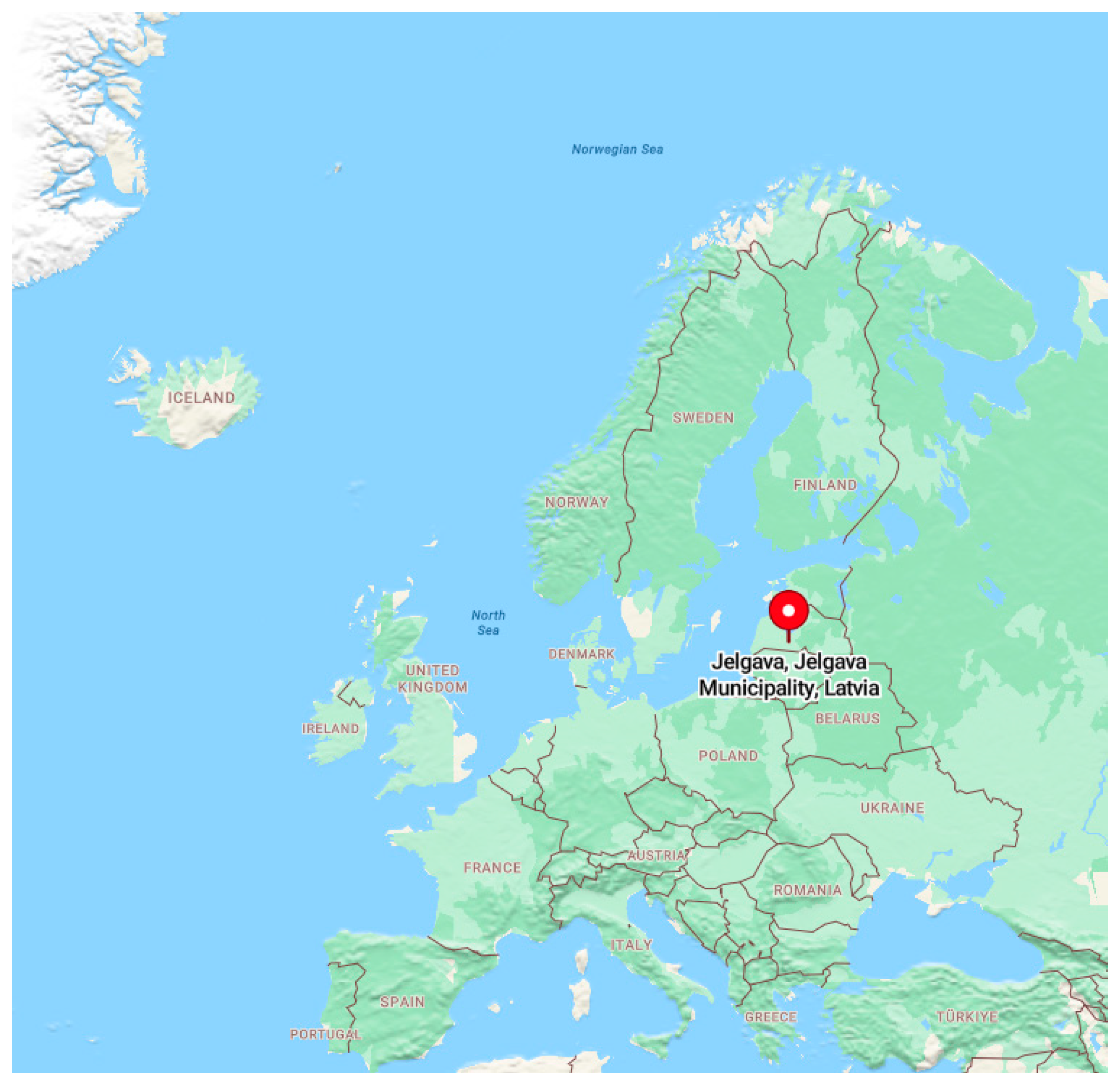
2.3. Defining a Case Study

The developed stock and flow models are applied for a case study exploring the scenarios of conventional and smart contract insurance. These scenarios are designed to test the effectiveness of smart insurance contracts for real estate assets in mitigating the impacts of climate change-related extreme weather events. The empirical data is collected for a local case study of Jelgava city (see Figure 1), which is located in central Latvia and has a population of around 55 thousand inhabitants.

The city is subjected to the yearly natural hazard of spring floods, and the insured assets considered in this study are residential buildings for the spring floods with a high probability (10% or once every 10 years), average probability (1% or once in 100 years) and a low probability (0.5% or once every 200 years) with losses and costs of restoration shown in

Table 1. Disaster probability, damage, and restoration costs (Latvian Environment, Geology and Meteorology Centre 2019).

Flooding Probability in 100 Years, %	Flooded Buildings Area, m2	Restoration Costs per m2
10%	103,773	19.5
1%	547,400	25.8
0.5%	695,111	31.8

.

This statistical data serves as an input for stochastic-probabilistic spring flood hazard event simulation implemented in the SD model trough function RANDOM (stochastic component), applying hazard probabilities with different return times (Feofilovs and Romagnoli 2021). The simulation includes a stochastic-probabilistic variable in the model and considers random sampling of 1000 simulation runs. This number of simulation runs is enough to capture a variety of possible combinations for disaster event occurrences over 50 years from the given disaster input data in Table 1.

The function describing asset loss is based on the damage curve for buildings from national flood risk assessment and management plans (Latvian Environment, Geology and Meteorology Centre 2019), and the insurance model is expressed in monetary units. The damage is accounted for in the damaged asset area (m²). The determined risk premium that insured assets must pay to an insurance company in the model simulation is estimated for a 10-year period by Equation (1):

$$RP=L_{average}+\sigma \ast P$$

(1)

where

• RP—Risk Premium,
• L_average—loss associated with the average yearly loss per asset in the area subjected to disaster,
• σ—volatility of yearly loss per asset in the area subjected to disaster,
  P—premium charge in %.

Three scenarios are compared with the help of the developed SD model in a simulation for a time period of 50 years and a time step of one year. The scenarios are summarized in

Table 2. Analysed scenarios with the developed SD model.

Scenario	Title	Risk Premium	DRR Measure	Flood Risk Reduction Measure Efficiency, %	Flood Risk Reduction Measure Cost, EUR
1.	Business as usual	Assessed every 10 years	No	-	-
2.	Investment in disaster risk reduction	Assessed every 10 years	Riverbed cleaning, coastal erosion prevention, and flow-through restoration	20.5	1,200,000
3.	Smart contract approach	Fixed	Riverbed cleaning, coastal erosion prevention, and flow-through restoration	20.5	1,200,000

Note: DDR—Disaster Risk Reduction.

and include:

(1)

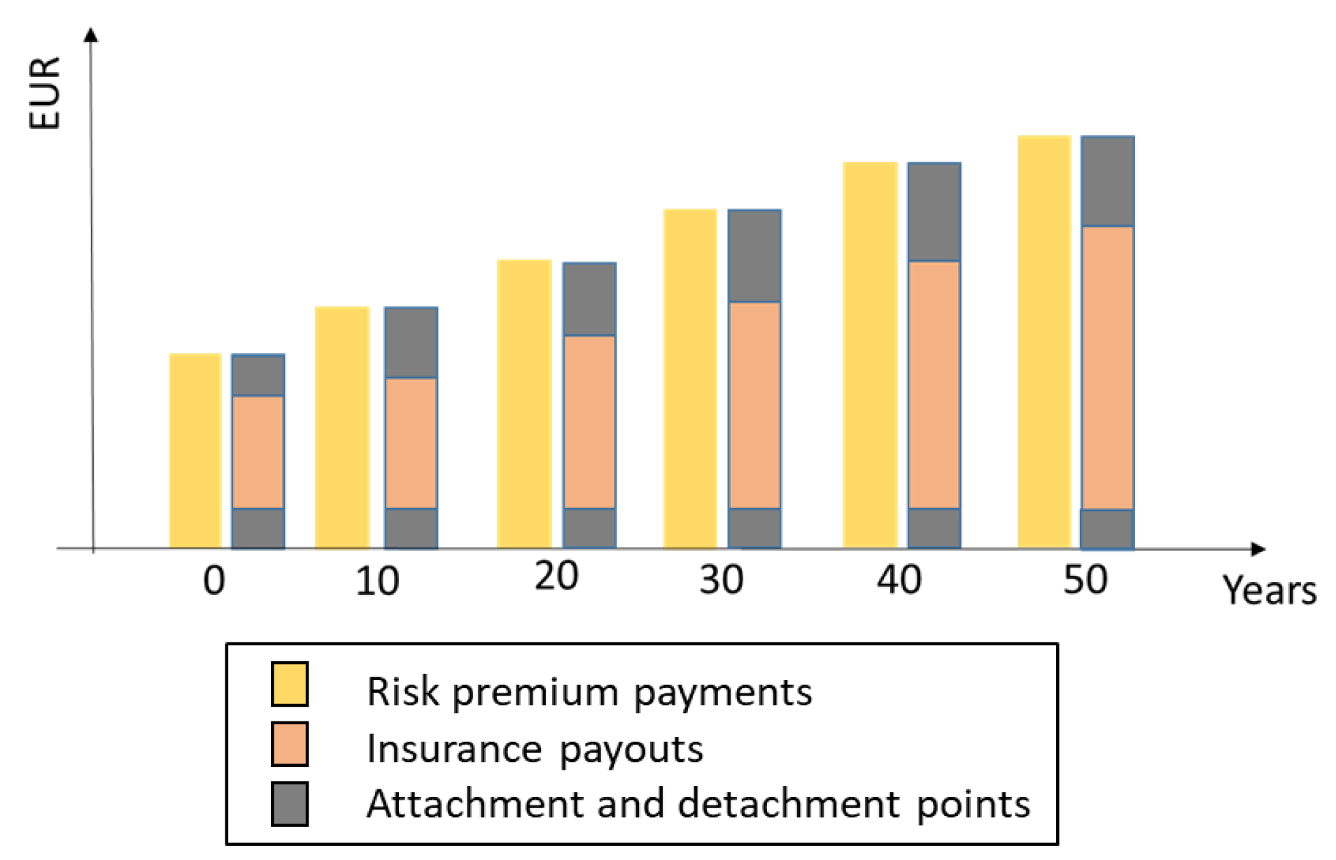
Scenario 1—Business as usual (BAU)—conventional insurance mechanism;

(2)

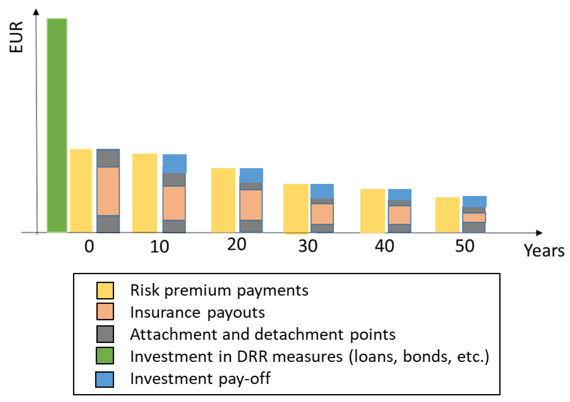
Scenario 2—Investment in disaster risk reduction—the insurance with bond for DRR measures without fixed premium;

(3)

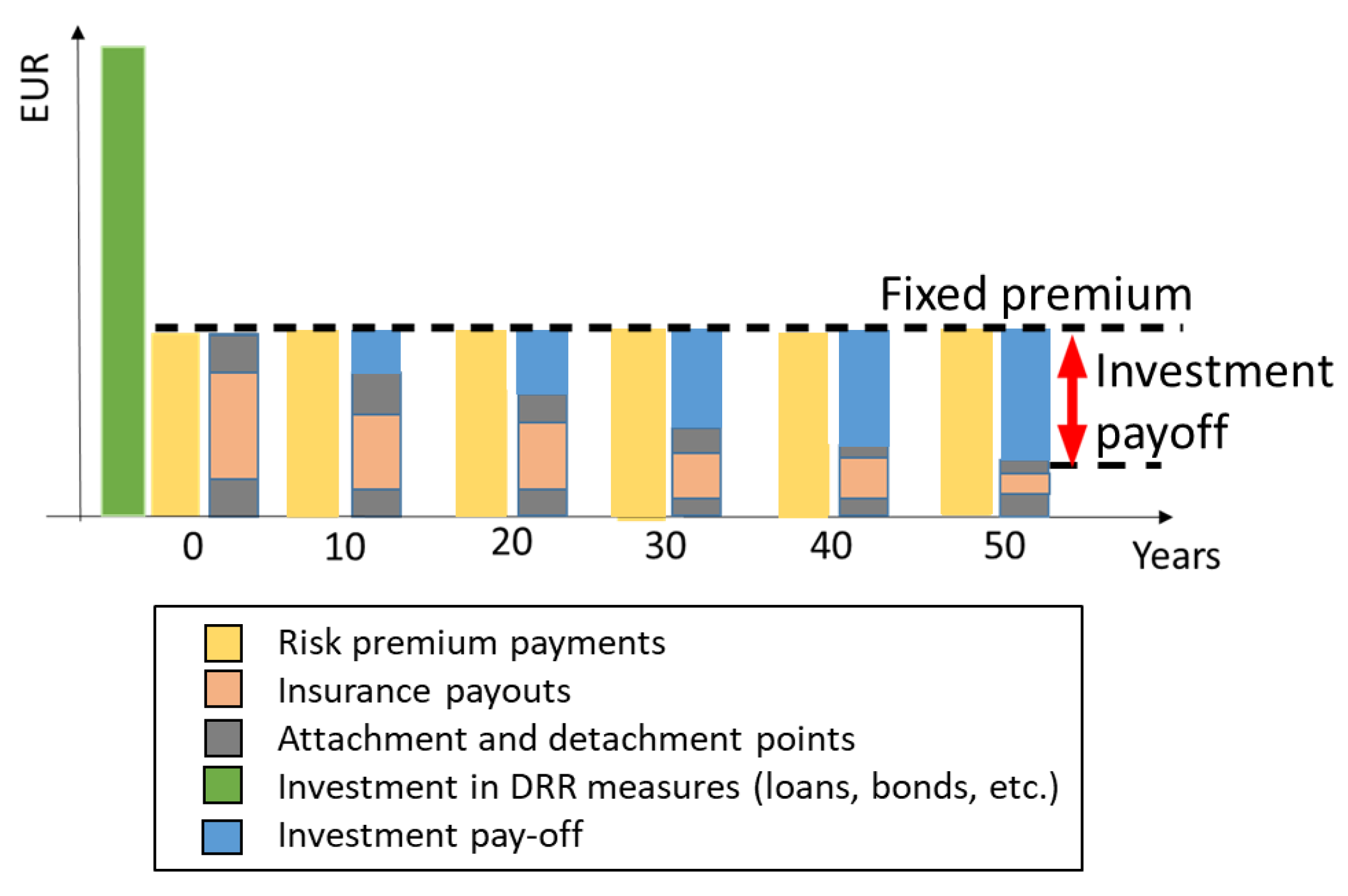
Scenario 3—Smart contract approach—the proposed smart contract insurance scheme with investment in disaster risk reduction (DRR) and fixed premium.

The Scenario 1 assumption is that the risk premium payments will increase because of an increasing number of insurance contracts, which occurs because of higher risk perception related to climate change. The expected behavior in risk premium payments and insurance payouts for Scenario 1 is illustrated in Figure 2 with payment flows of a 10-year period. The attachment point is the level of loss at which the insurance company will step in to pay for the excess losses, and the detachment point is the level of loss that will no longer be covered by the insurance company. The payouts to insured assets are being made in the amount that is between the attachment point and detachment point of insurance, meaning the risk behind the points is not covered.

The proposed Scenario 2 and Scenario 3 approaches foresee an investment made by the government into DRR that will positively affect the safety of the insured assets. The idea of these scenarios is that the insurance company accepts the obligation in the form of bonds to pay the government’s investment, moving towards a proactive role of the insurance sector as a driver for risk mitigation and prevention measures. The government is considered the representative of the local area that is responsible for fostering the DRR and, therefore, is interested in investment in DRR that is eventually paid off by an insurance company through bonds.

Such an approach considers that the risk is reduced because of the effective implementation of DRR, and consequently, the insurance payouts will reduce because of fewer events encountering damage to assets, also leading to the decrease in the risk premium accordingly. This case is described by Scenario 2 and presented in Figure 3.

Though this is a practice towards the reduction of DRR, in certain cases, a negative balance in the insurance company budget may occur when a decrease in risk premium payouts because of a decrease in disaster events leads to an inability to cover the initial investment into DRR, hence there must be introduced a fixed premium price. The case of a fixed premium is considered in Scenario 3, shown in Figure 4, and named the Smart contract approach. Within this approach, the share of insurance companies’ income, which is the difference between insurance payouts and the fixed risk premium, is used to pay off the bonds of the initial investment in the DRR measure made by the government.

The total expenditure of the company in Scenario 1 is different from the Scenario 2 and 3 approach, where the insurance company expenditure is not only the payouts to insured assets after damage has occurred but also the pay-off of investment. The insurance companies’ expenditure can be used to compare the overall costs of moving from the conventional insurance scheme in the BAU scenario towards the Smart contract approach, and in the SD model, is estimated as the sum of payouts to insured assets after the damage has occurred and the pay-off of investment. Also, the total disaster costs are estimated to compare the overall effectiveness of studied scenarios as the sum of the damage to all the assets in the area and investment into DRR measures.

The DRR measures in Scenarios 2 and 3 are selected based on the assumption for Jelgava city flood management plans and are presented in Table 2. The study considers that under the given flood risk reduction measure, there falls not only the insured assets but also other assets in the area when flood risk reduction measures are implemented. The effect of such an approach toward investment in DRR can lead to a decrease in the risk and the risk premium; hence, the willingness to pay for insurance can increase. The developed SD model allows the simulation of the change in the number of insured assets in the area. The assumption in a case study for the initial share of insured buildings in the area is equal to 10%. In reality, the change in number of insured assets is influenced by such factors as perception of risk and willingness to pay for the risk. However, the perception of risk is not further studied in the model. The changes in willingness to pay for the risk parameter are tested through sensitivity analysis in order to understand the influence of the variable on the model’s output.

Another assumption in the model for the company’s profit is that it does not consider payments for workers and other expenses related to the administrative processes. Only risk premium payments are accounted for as income, and the payouts with investment pay-off as outcomes. The difference between income and outcome is considered as the insurance companies profit.

2.4. Model Testing and Validation

Multiple structure verification experiments were conducted in order to validate and verify the developed System Dynamics model. The tests to check the model’s structural soundness and gauge how well it captured the system’s behavior in various scenarios included a number of methods. The model was simulated to see if it could replicate the foreseen behavior of a system after the initial stock, and parameter values were estimated using available data and expert knowledge.

2.4.1. Content Validation Procedure

A thorough validation process was used to evaluate the model’s content validity, and a panel of subject-matter experts in climate change, insurance, and system dynamics modeling. The experts reviewed the model’s structure, assumptions, and parameters as part of the process. The validation procedure was conducted in several stages. First, the model CLDs were presented to the panel for review, and feedback was solicited on the model structure and assumptions. The panel provided input on the key variables and interrelationships in the model and suggested changes to improve the accuracy and robustness of the model. Next, the model parameters were reviewed by the panel. The experts provided feedback on the values and ranges of the parameter values and suggested changes based on their expert knowledge and available data.

2.4.2. Extreme Value Test

The SD model is validated through an extreme value test, in which the model is calibrated using historical data from the case study and then simulated with extremely high and low parameter values to understand if the model behavior is logical to the assumptions made in CLD and SD stock and flow model under extreme condition. The test involves comparing the model predictions to extreme changes in model variables and Hazard occurrence. For extremely low-value tests, the hazard occurrence was set as no hazard during the simulation period, and the area of assets with insurance was equal to all the assets in the area. For the extremely high-value test, the Hazard occurrence is set to the occurrence of the hazard with maximum damage every simulation year with all the assets insured. In addition to these changes for both extreme value tests, also the Area of assets with insurance variable is set to be equal to all asset areas in the selected case study, and the Exhaustion point (e.c. Detachment point) of insurance payouts is set to 0, meaning all losses will be covered by the insurance company.

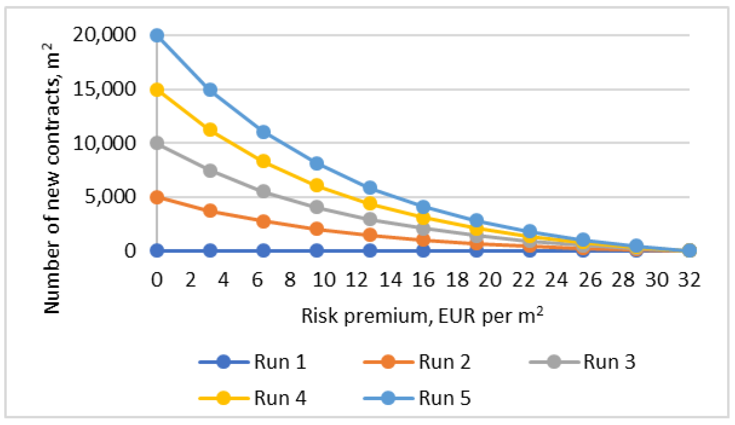
2.4.3. Sensitivity Analysis

Understanding the effects of model uncertainty and identifying the crucial variables that have the biggest impacts on the model’s output is important for further use of the model in practice. In this case, sensitivity analysis is used to analyze how a system responds to changes in the values of one or more input parameters, the data of which is uncertain, but the variable may be crucial for model output.

In this study, a sensitivity analysis is conducted by testing the effect of one specific parameter influencing the number of insured assets because it is an important factor for the overall output of the model regarding the risk premium payments and payouts for damage to assets. The Willingness to pay for insurance in the model is determined by the number of new contracts based on Risk Premium cost. The number of new contracts in the model is based on the hypothetical functions presented in Figure 5, where risk premium is measured in EUR per m² and Number of new contracts in m² (new insured area of assets). In total, five simulation runs are made in sensitivity analysis with different hypothetical functions for the number of new contracts.

For sensitivity analysis, the hazard event is kept static as in an extreme value test with maximum hazard occurrence possibility to obtain comparable results over several sensitivity analysis simulation runs.

3. Results and Discussion

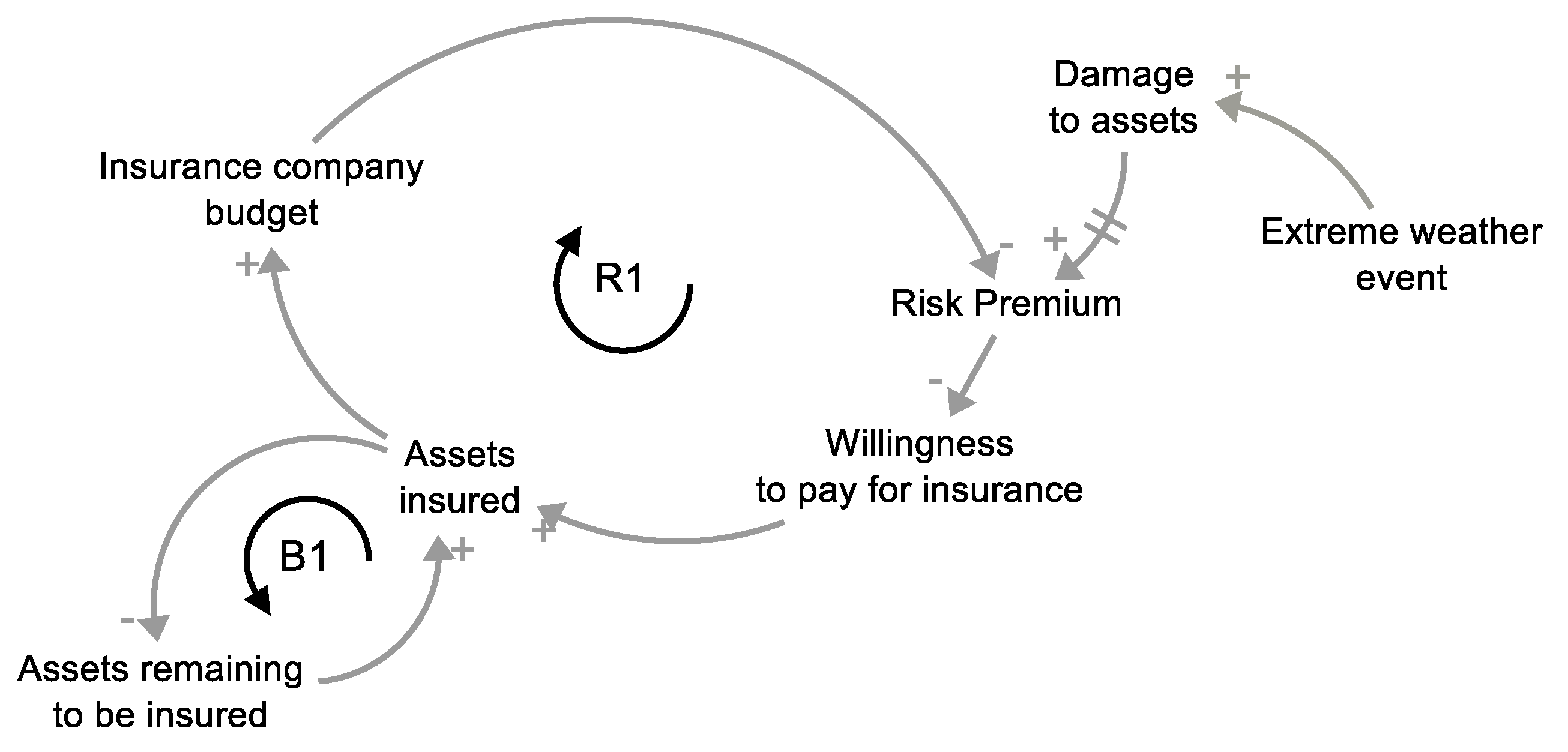
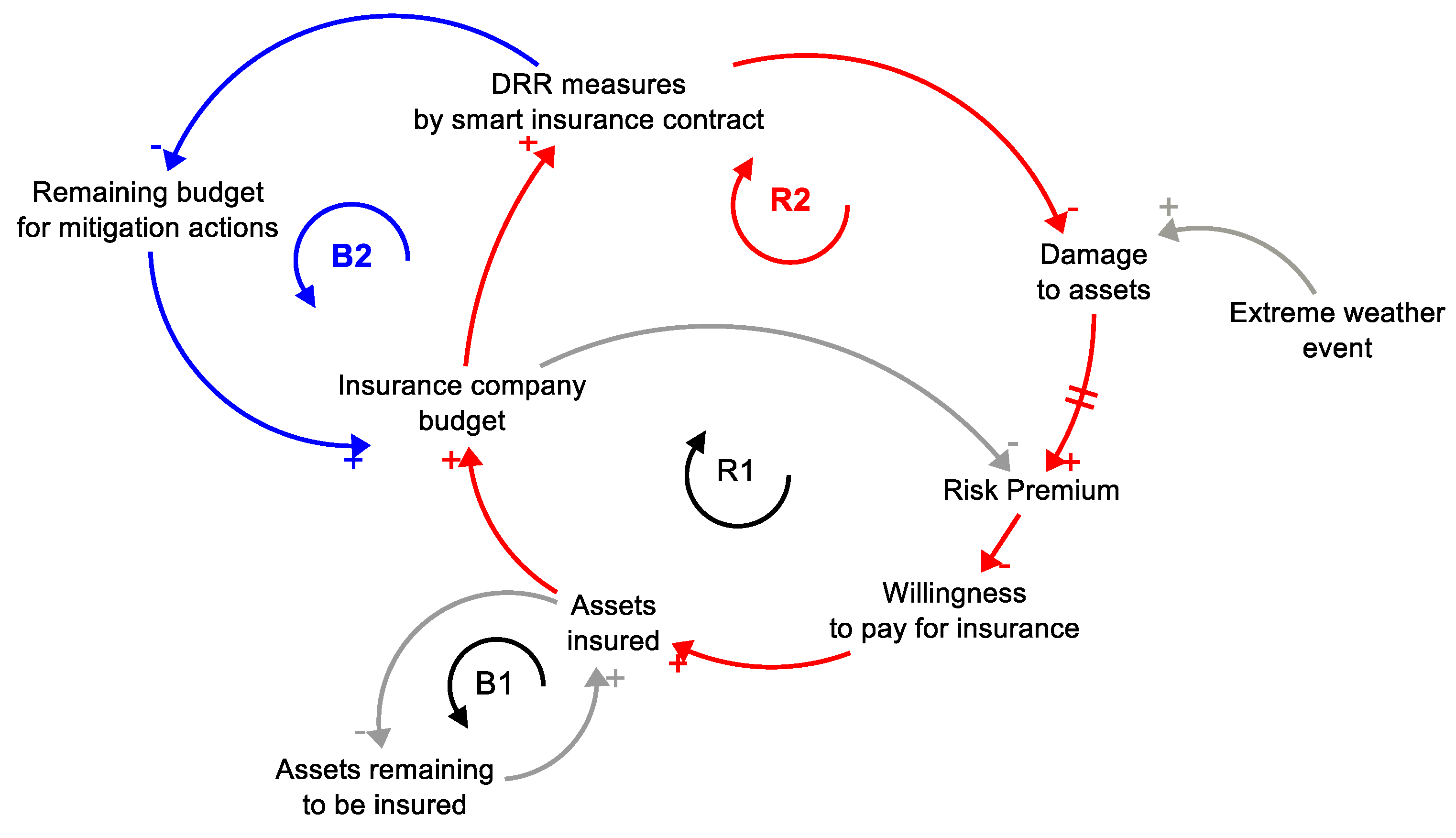
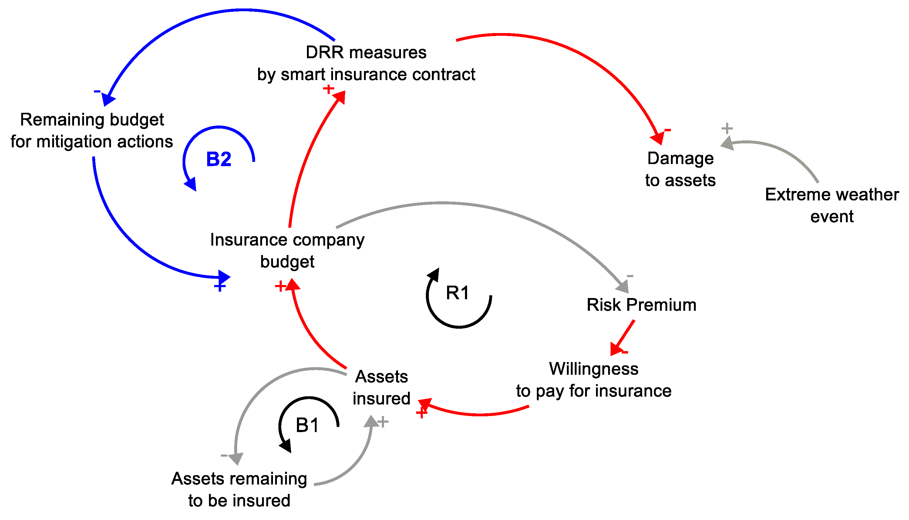
3.1. Causal Loop Diagrams of the Developed Model

The behavior of the studied insurance mechanism implemented in the SD model is explained through CLDs shown in Figure 6, Figure 7 and Figure 8 and shows only the main variables important to explain the dynamic behavior of the SD model.

The BAU scenario CLD in Figure 5 consists of two feedback loops and the out variable of Damage to assets and Extreme weather events. The links between variables show that an increase in Extreme weather event variable value will lead to an increase in Damage to assets value, under the assumption of “all other things being equal”. Applying the same assumption, the increase in Damage to assets will lead to an increase in Risk Premium value. The two stripes on the connector between Damage to assets and Risk Premium symbolize the time delay between the accounted damage to assets over a period of time for which the risk premium is estimated.

The variables connected in the reinforcing loop R1 are Risk Premium, Willingness to pay for insurance, assets insured, and the insurance company’s budget. The reinforcing loop R1 is a positive loop, meaning that there is an increase of values in the variables connected in the loop. This loop represents the dynamic problem of increasing Risk Premiums over time with the increase of damage to assets that leads to the growth of the insurance company’s budget and, thus, a decrease in Risk Premiums, as introduced in Figure 2. In this case, the strength of the decrease in Risk Premium value depends on the supply-demand elasticity function. The growth in loop R1 depends on the number of assets in the area, and CLD is marked with balancing loop B1, which includes variable insured assets and assets remaining to be insured.

Two more feedback loops are added to Scenario 2, including the investment in disaster risk reduction (Figure 7). The loop R2 shows how investment in DRR measures by smart contract will lead to a decrease in Damage to assets, thus a decrease in Risk Premium and consequently an increase in Willingness to pay for insurance, assets insured, and insurance company budget. Loop B2 is the balancing loop of reinforcing loop R2, which does not allow infinite growth in the insurance company budget.

To implement a smart insurance scheme, it is necessary to cancel the effect of loop R2 in the given insurance system model by introducing a fixed premium that does not depend on the damage to assets and is determined based on the historical data at the moment when it is fixed. Therefore, in Figure 8, the CLD showing the smart contract approach does not include the link between damage to assets and risk premium. The panel of SD and insurance experts reviewed and approved the proposed CLD for further implementation in an SD stock and flow model.

3.2. Empirical Model Testing and Validation

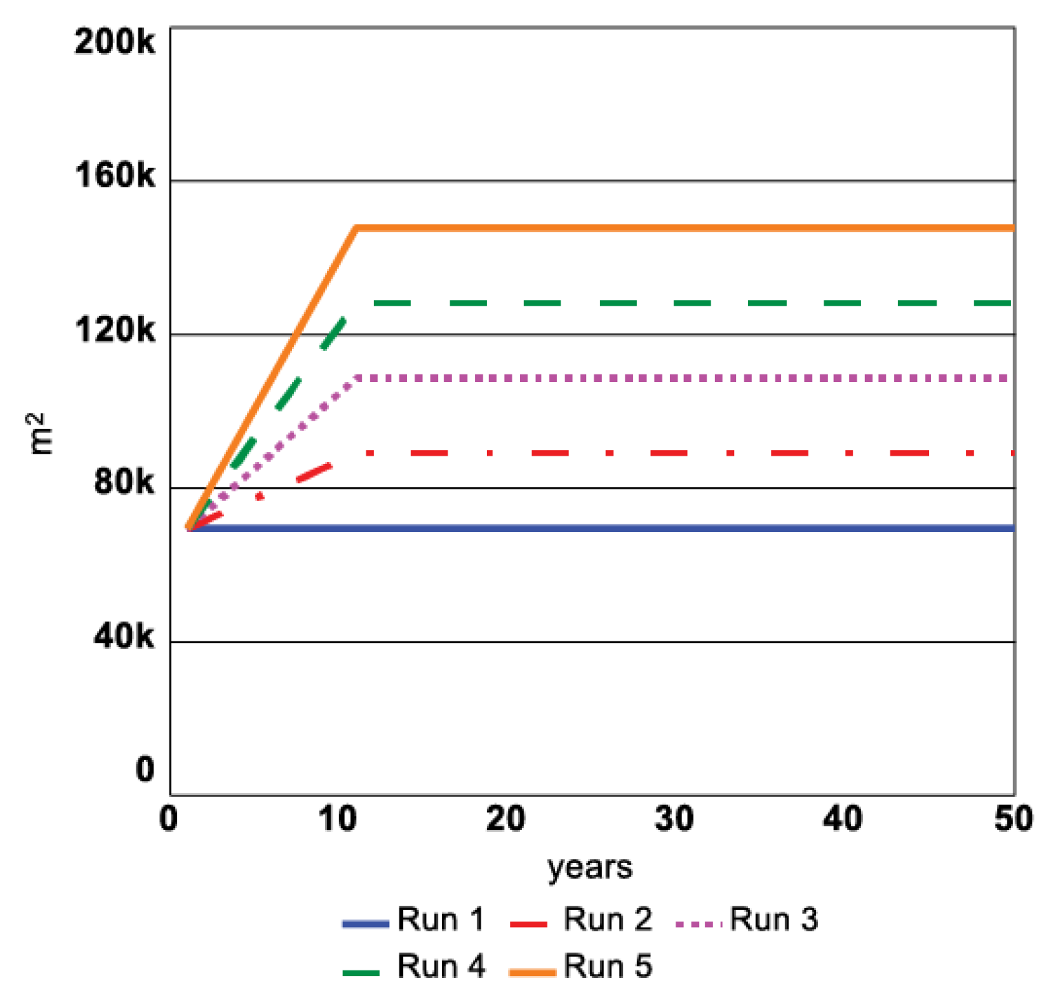
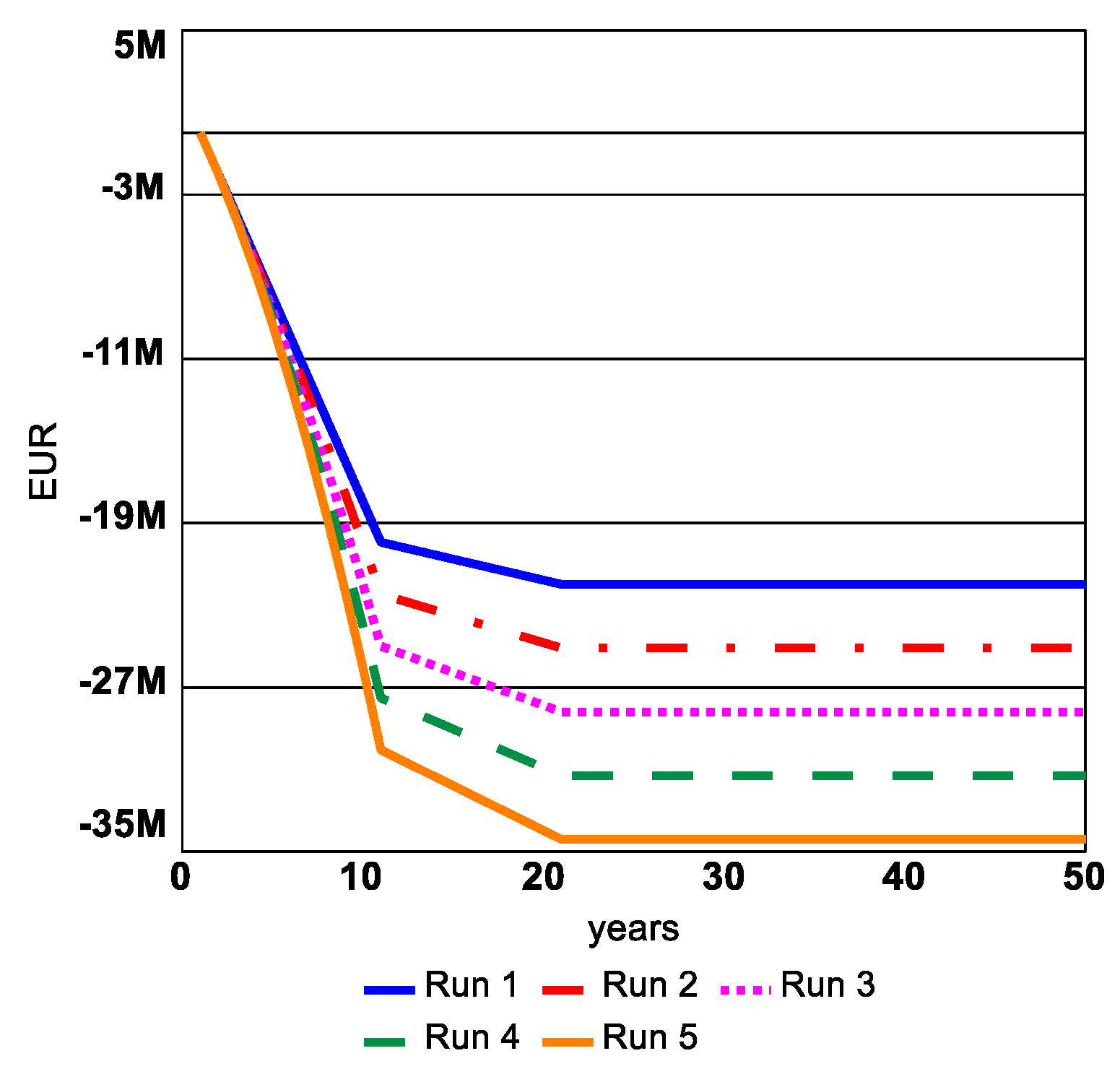
3.2.1. Results of Extreme Value Test

Model testing by extreme value test is performed for Hazard occurrence variable into separated simulations with minimum and maximum values of hazard event magnitude (i.e., Flooded buildings area, m²) set for each simulation step. This simulation result for the risk premium variable in Figure 9 shows a decrease of the value to 0 over the simulation time because of no risk of a hazard event.

The behavior of the risk premium variable corresponds to the variables shown in Figure 10. The values of variables shown in Figure 10 are cumulative values in a given simulation step. The increase in the insurance company’s profit occurs due to received risk premium payments in the first 10 years of simulation, considering that there are no damage costs to cover. In this case, the risk premium is still based on historical risk statistics. In the next ten simulation years, the risk premium is decreased due to a decrease in risk as the hazard occurrence variable is set to zero. Consequently, the insurance companies’ profits are growing slower. The rest of the simulation period after simulation year 20, when the risk premium is equal to zero, and the profit of the company has reached a plateau.

The result of the extreme value test with hazard occurrence variable maximum value is presented in Figure 11 for the Risk Premium variable and Figure 12 for Insurance company profit, Total costs of disaster, and Total damage costs covered by insurance.

The results show an increase in Risk Premium after 10 years of simulation due to increased risk of hazard and another increase after 20 years of simulation. Further growth does not occur as the Risk Premium value has reached a plateau in regard to the maximum risk of hazard. The Insurance company’s profit appears to be negative, meaning that the insurance company experiences financial losses in case of extremely high-hazard event occurrence. Consequently, the total costs of disaster and the total damage costs covered by insurance increase over simulation and have the same value as all of the assets in the area considered insured for extreme maximum value test (see Figure 12). The Extreme value test results show that the model behavior is logical to the assumptions made in the CLD and SD stock and flow model.

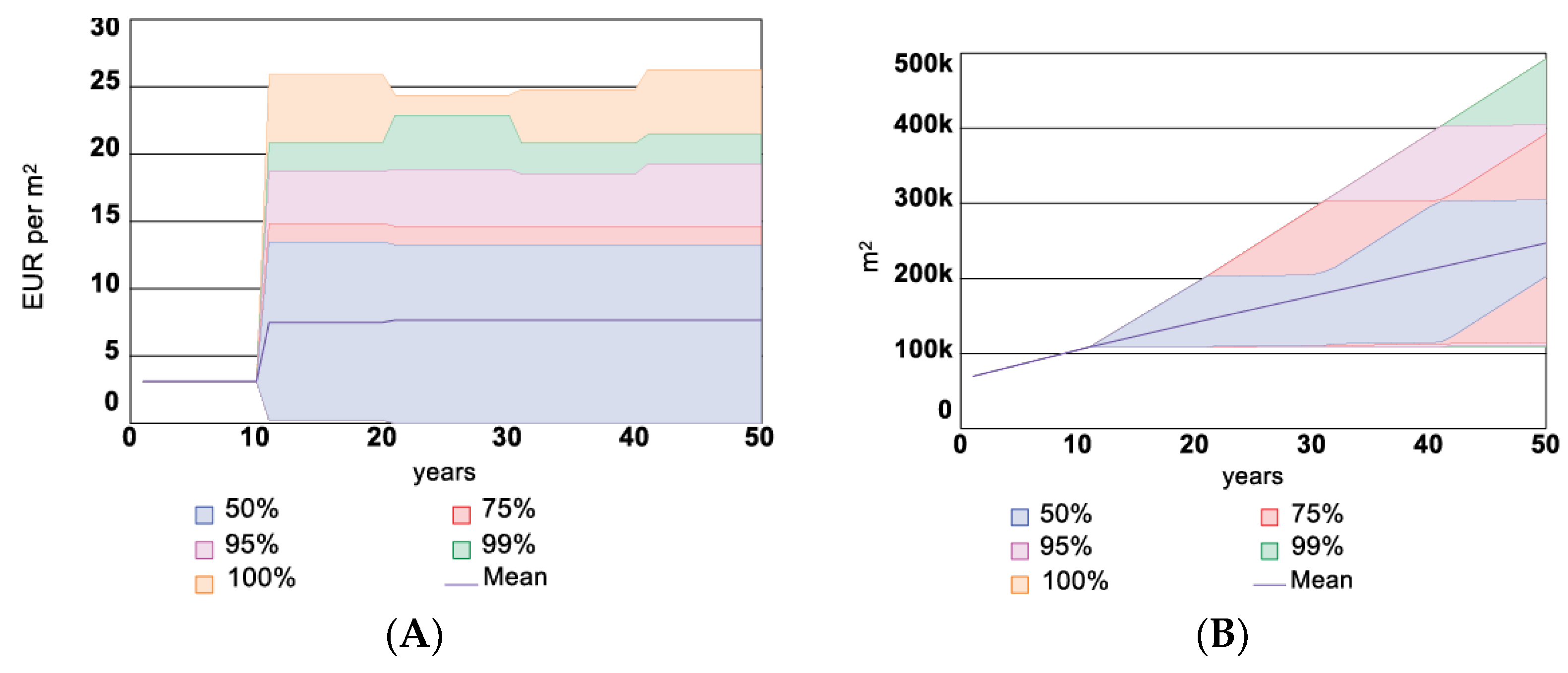
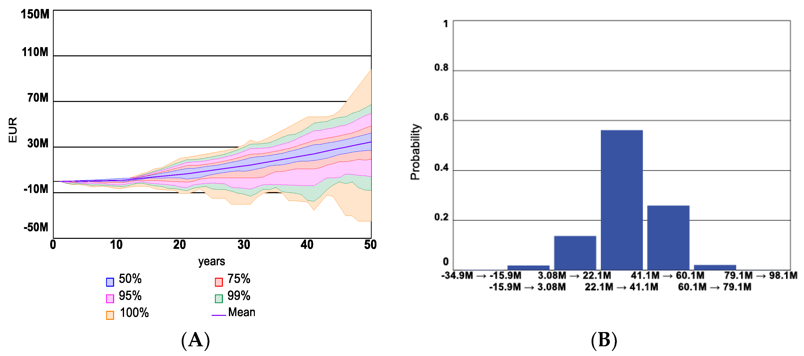
3.2.2. Sensitivity Analysis Output

The results of the sensitivity analysis show that the model is sensitive to changes in the Number of newly signed contracts variable. Figure 13 shows how the assets with insurance variable, measured as the area of assets with insurance in m² units, changes under assumptions of hypothetical function for the Number of newly signed contracts variable shown in Figure 4. Simulation run 1 considers that no new contracts are made, and therefore, the area of insured assets remains the same. In further simulation runs, the sensitivity of willingness to pay for insurance is increased, and therefore, for each simulation run, more new assets sign insurance contracts.

The hazard occurrence is maintained at the maximum possible, and the Risk Premium value remains the same as introduced in Figure 11. The Area of assets with insurance in Figure 13 after the simulation year 10 reaches a plateau as no new contracts are signed due to the increase in Risk Premium. Moreover, Figure 14 shows that insurance company profit under sensitivity analysis corresponds to the expected logical behavior of the model. The figure shows how a higher number of contracts will lead to higher losses in insurance companies’ budgets because of higher payouts for damage under extremely high hazard occurrence every simulation year compared to the historical hazard occurrence at the start of the simulation. Again, the results of sensitivity analysis show that the model behavior is logical to the assumptions made in the CLD and SD stock and flow model.

3.3. Results of Case Study and Policy Scenarios

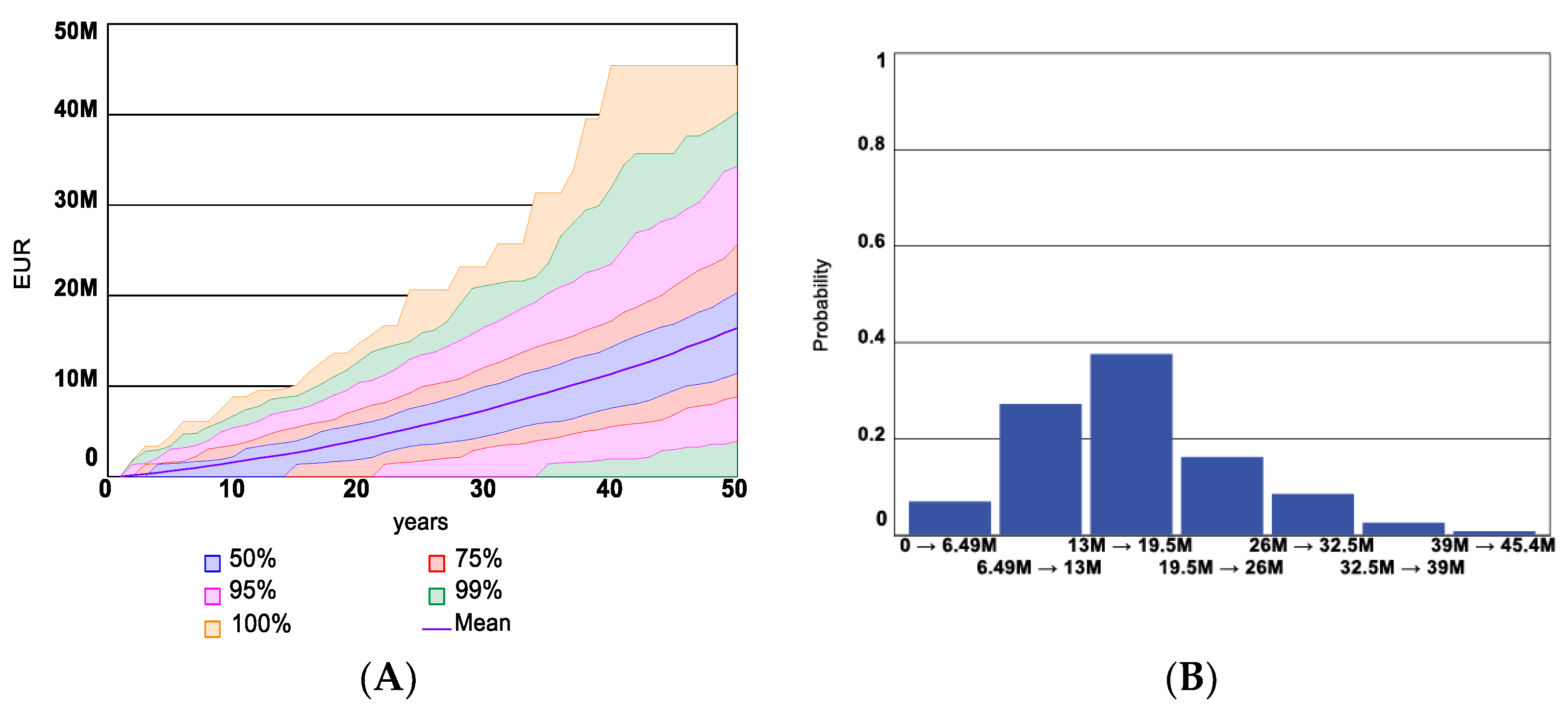
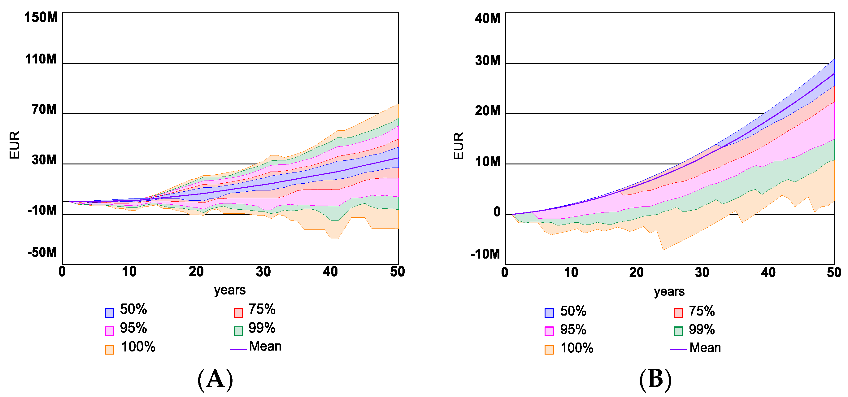
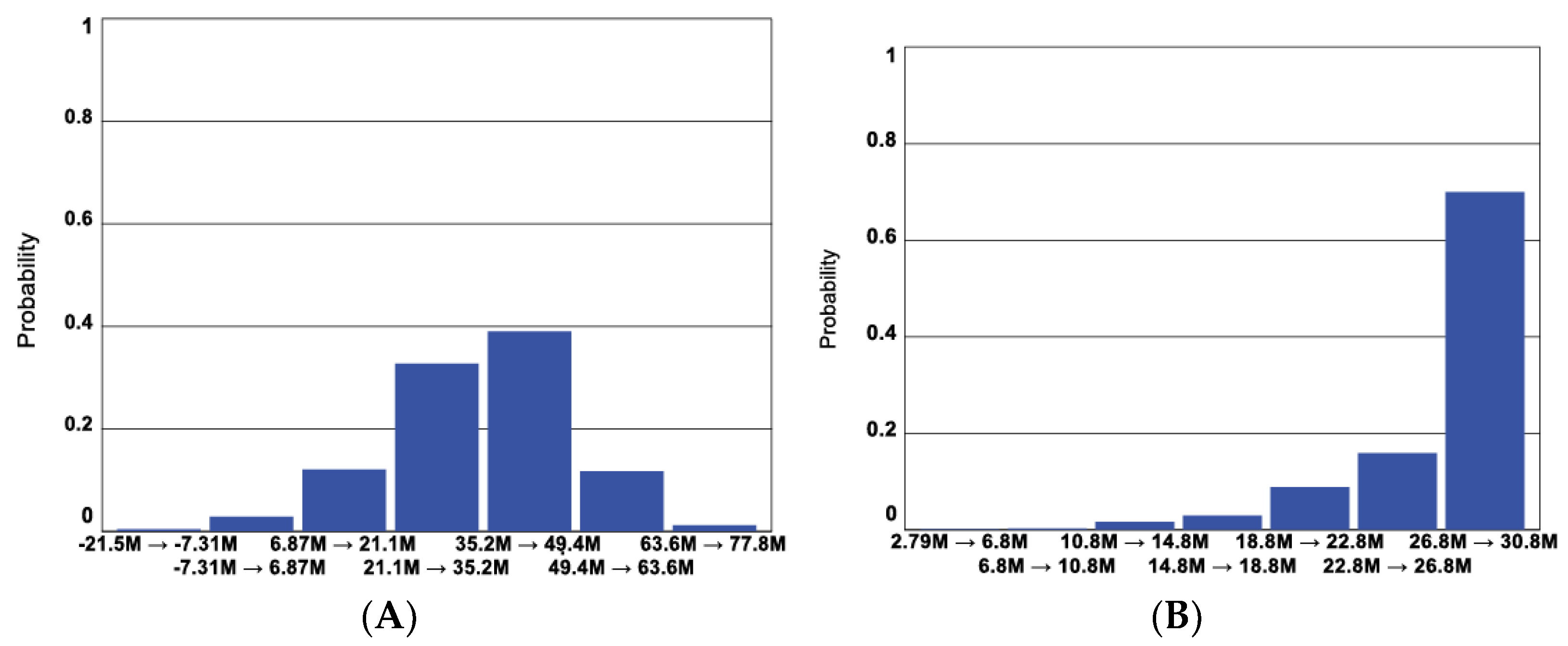
3.3.1. Business as Usual Scenario

The results obtained for the risk premium in the BAU scenario shown in Figure 15A indicate that the average mean value for the risk premium value in all simulations increases compared to the historical risk premium at the start of the simulation. Nevertheless, the Risk Premium value in all simulations leads to an increase in the Area of assets insured value by the effect of the hypothetical function for the Number of newly signed contracts variable, as shown in Figure 15B.

The mean average simulation runs for insurance companies’ profits in the BAU scenario shown in Figure 16A increase during the simulation period. However, simulation results appear as negative values in insurance company profit for simulation with the most frequent occurrence of hazardous events. The probabilities of the final insurance companies’ profits at the end of the simulation run are shown in Figure 16B.

The confidence intervals and histogram for Insurance companies’ expenditure in the BAU scenario are shown in Figure 17A,B, respectively. In the case of the BAU scenario, the damage costs covered by the insurance company due to insurance payouts for insured assets are equal to the total insurance companies’ expenditure.

The Total costs of disaster for all assets in the area (see Figure 18) appear to be much higher than the Damage costs covered by the insurance company in Figure 17. This is due to the fact that at the start of the simulation, only 10% of assets in the area are considered to be insured, and during the simulations, a relatively small share of the total assets area is signing insurance contracts based on Hypothetical functions for the Number of new contracts variable, which is dependent on risk premium value, which again is dependent on the hazard occurrence over the simulation period.

The results of the BAU scenario can be interpreted in the following way according to the CLDs: the occurrence of disaster events during the simulations is higher than historical, and therefore, the Risk Premium is increasing, and the Area of assets insured value by the effect of hypothetical function for Number of newly signed contracts (Figure 15) therefore the Insurance company profit is also increasing (Figure 16). Nevertheless, Damage costs covered by insurance companies (Figure 17) and the Total costs of disaster (Figure 18) are increasing significantly over simulation time. The results of the BAU scenario underline that the model represents the dynamic problem of existing disaster insurance mechanisms defined for the study.

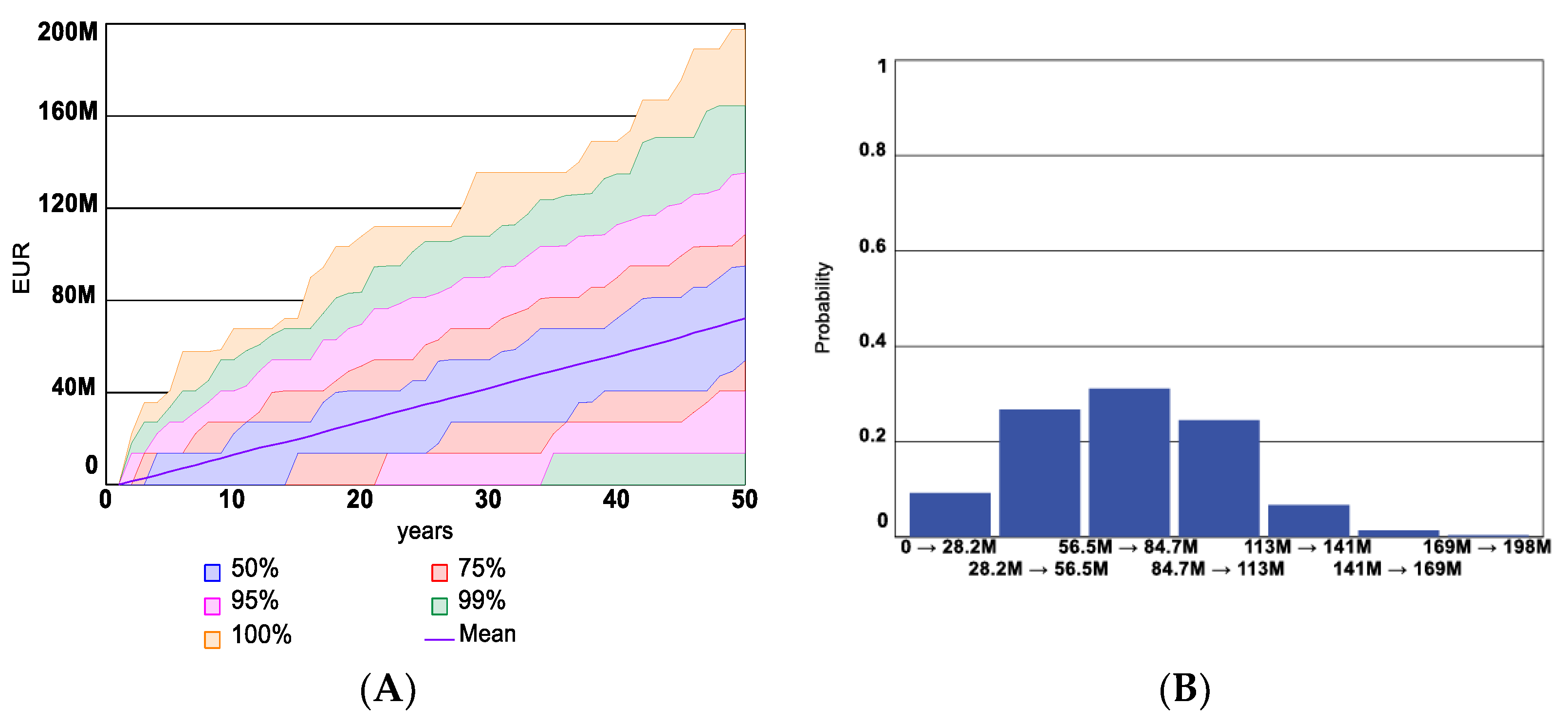
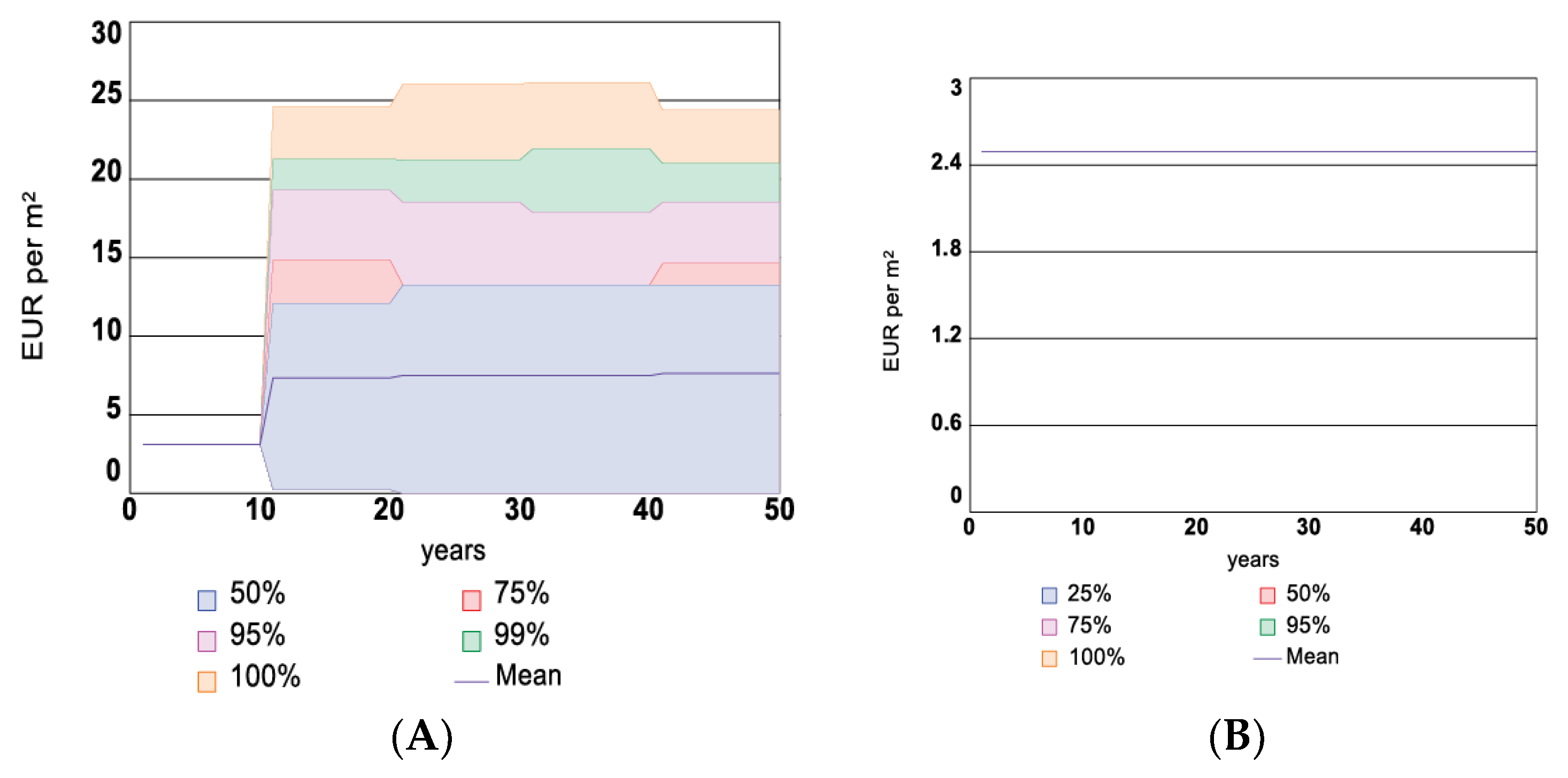
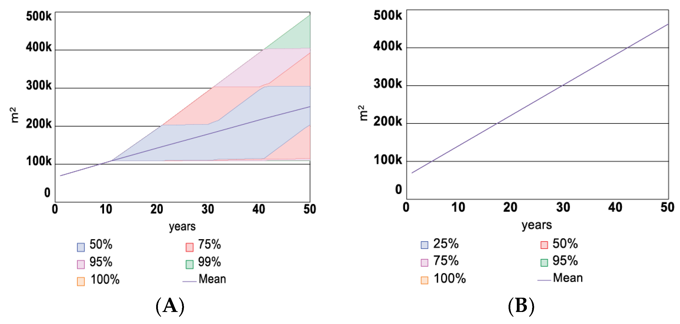
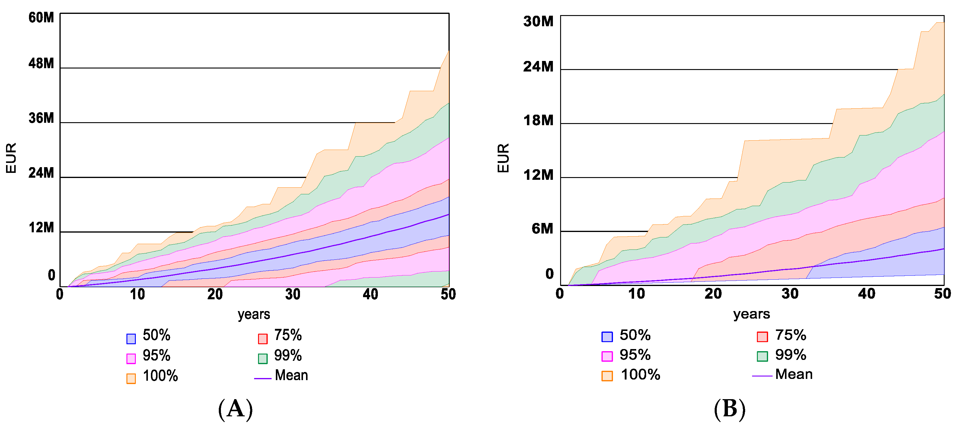
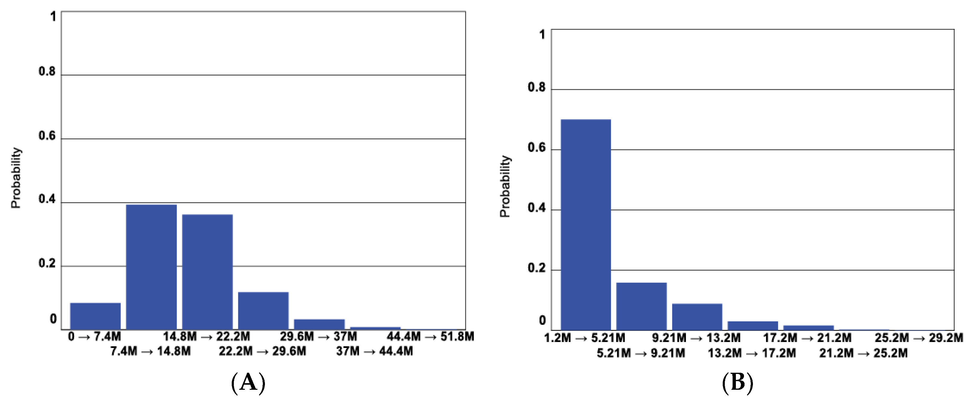
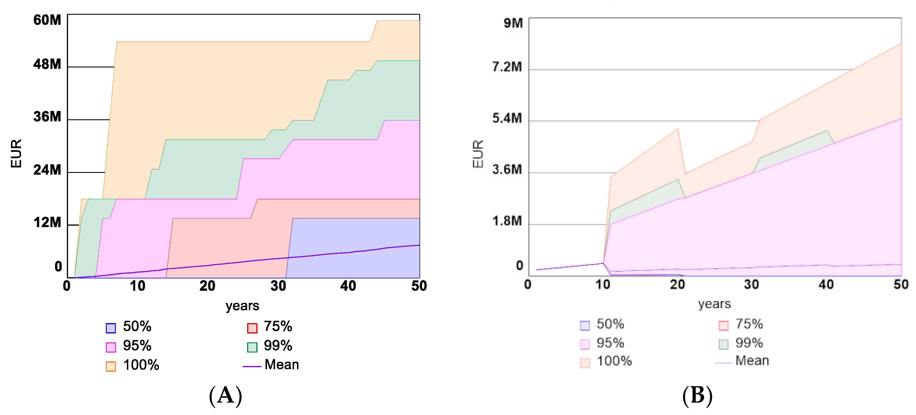
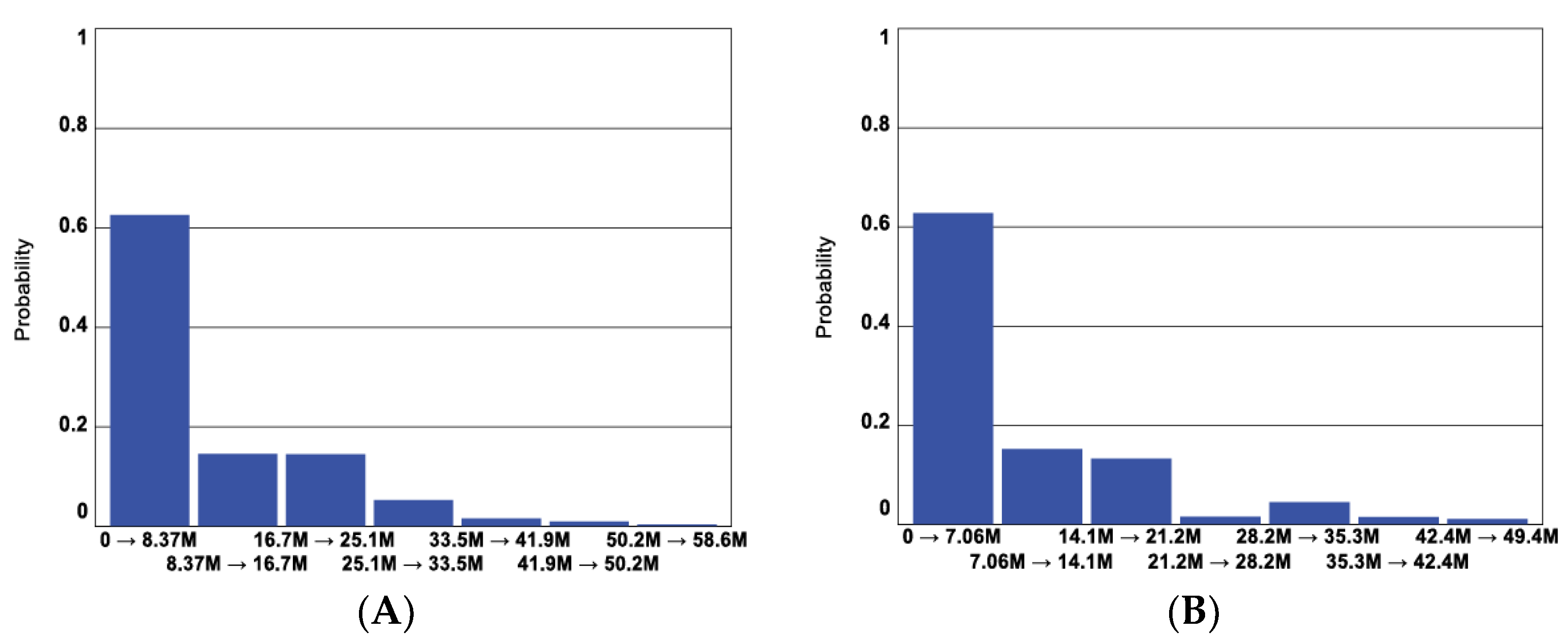
3.3.2. Scenarios with Investment in Disaster Risk Reduction

The results of the simulation for Scenario 2 with investment in flood risk reduction measures in Figure 19A show the confidence intervals for the Risk Premium, which is similar to the BAU scenario output. In Figure 19B, the Risk Premium for Scenario 3 is given as static according to the definition of the fixed Risk Premium value in all 1000 simulation runs.

In Figure 20A,B, the corresponding tendency of the number of insured assets is shown for Scenario 2 and Scenario 3, respectively. Scenario 2 has a variation in the number of insured assets corresponding to a variation in the Risk Premium, while Scenario 3 has the same trend in all simulations due to the fixed premium definition.

The results of the Number of insured assets in both scenarios with investment in DRR are shown in Figure 21. Scenario 2 (see Figure 20A) has a similar tendency in confidence intervals to Scenario 1 (See Figure 20A), showing that the investment in flood risk reduction measures will lead to a slight decrease in the variability of insurance company profit. For Scenario 3 (Figure 20B), the confidence intervals for the Insurance company profit show that the range of profit uncertainty has decreased, and most of the simulation results are located at the higher levels of the graph with the mean average of the simulation outputs is moved closer to the higher income values. There are also fewer probable outcomes with negative insurance companies’ profit values. The distribution of Insurance company profit in Scenarios 2 and 3 in the form of Histograms is shown in Figure 22A,B, respectively.

Though there is a certain probability of having a higher company profit in Scenario 2thann in Scenario 3, the total Expenditure of the insurance company on disaster, including the damage-related payouts and pay-off of investment in Figure 23 and Figure 24, shows how Scenario 3 leads to lower overall expenditure and maintains very high probability of having low the average mean of the payouts. This signifies that Scenario 3 has the overall lowest costs in all scenarios compared, while Scenario 2 is slightly better than business as usual in Scenario 1.

Finally, the Total costs of disaster are compared in Figure 25 and Figure 26. The results show that Scenario 3 leads to much lower total disaster costs thanks to fixed premiums. As for Scenario 2, the total costs of disaster appear slightly lower than those shown for Scenario 1.

3.4. Discussion on Findings and Limitations of the Case Study Results

The findings of this study underscore the efficacy of innovative insurance mechanisms in mitigating climate change-related disaster risks, aligning with prior research advocating for proactive risk management strategies. Unlike traditional models that focus on post-disaster financial recovery, this study introduces a mechanism that emphasizes risk prevention and mitigation, echoing the call for more forward-looking approaches in the insurance sector. This aligns with the growing body of literature that supports the integration of risk reduction measures into insurance frameworks to enhance resilience against natural disasters. This study contributes to the evolving field of disaster risk management by proposing an innovative insurance mechanism tailored to the challenges posed by climate change. It calls for a shift from traditional, reactive insurance models to proactive, prevention-oriented strategies, offering a blueprint for enhancing resilience and sustainability in the face of increasing disaster risks.

Latvia’s insurance policy landscape for natural disasters is characterized by a need for innovative approaches to managing increasing risks due to climate change. The study highlights Latvia’s vulnerability to flooding and the potential economic impacts of climate-related events on urban resilience. By implementing the proposed innovative insurance mechanism, Latvia can move towards a more proactive disaster risk management model. This approach not only aims to reduce immediate disaster costs but also contributes to the long-term resilience of communities, aligning with global trends towards sustainable and resilient urban development.

The study’s main limitation lies in its localized context, focusing on a case study in Latvia, which may not fully represent other geographic or socioeconomic settings. Future research should aim to apply the model in diverse environments to validate its universal applicability and effectiveness. Additionally, exploring the long-term sustainability of the proposed insurance mechanism and its adaptability to changing climate conditions and disaster risk profiles would provide valuable insights.

4. Conclusions

Insurance mechanisms that decline and mitigate climate change-related disasters play a key role in protecting lives, livelihoods, and infrastructure. Through robust risk assessment, innovative insurance mechanisms, incentives for risk reduction, capacity building, stakeholder collaboration, and continuous monitoring and evaluation, these mechanisms enhance community resilience and foster sustainable development in the face of climate change challenges. As climate risks continue to evolve, it is imperative to foster ongoing innovation, research, and policy support to ensure the effectiveness and accessibility of insurance mechanisms in the future.

The study highlights the usefulness of the System Dynamics modeling approach for examining the feedback loops that govern the behavior of complex systems related to the disaster insurance mechanism. The study aims to solve an existing problem in conventional disaster insurance mechanisms, which aims only to provide financial safety for asset recovery after a disaster event and not to decrease the risk of the disaster itself. This problem is especially becoming topical with climate-related disaster risk increases and can lead only to higher damage costs in the long term.

In this study, a new insurance mechanism is suggested to overcome the current ineffectiveness of the conventional insurance model in dealing with the growing threats of disasters, and it is applied in a local case study. For the proposed insurance mechanism, a dynamic hypothesis is created that foresees a smart insurance contract supporting investment in disaster risk mitigation measures to reduce damage costs, thus protecting insured assets and, at the same time, allowing new assets to be insured thanks to a more effective insurance scheme resulting even in higher benefits for the assets insured. The model’s structure is described by the causal loop diagrams and implemented in a stock and flow model, in which content is validated by experts and tested by extreme value tests and sensitivity analyses to verify the reliability of the model outputs.

The results of the extreme value test indicated that the model can accurately show the system’s behavior under extremely high and low variable values. This increases confidence in the model’s ability to predict the behavior of the studied system. The sensitivity analysis also showed that the model is sensitive to small changes in a single variable value. It is important to notice how these small changes can significantly affect the long-term behavior of the studied system under different inputs. Sensitivity analysis showed how a change in willingness to pay for insurance would influence the expected outcomes of the model. Overall, these structure verification tests provided important validation of the system dynamics model and increased confidence in its ability to accurately represent the behavior of the system under different conditions. By verifying the model structure, parameters, boundaries, extreme conditions, and unit consistency, the model was able to provide more accurate predictions and insights for the defined case study scenarios.

The case study was made for three comparative insurance scheme scenarios. Scenario Comparison in the case study showed that business as usual could lead to increasing risk premiums over time due to higher disaster event occurrences, leading to increased insurance company profits but also significantly higher disaster and damage costs. A scenario with investment in disaster risk reduction led to a decrease in insurance payouts because of fewer disaster events occurring, suggesting a better outcome than business as usual but with limitations on consistent revenue for insurance companies. The Smart Contract Approach scenario introduced a fixed risk premium and investment in DRR measures, demonstrating the lowest overall disaster costs and expenditure for insurance companies, indicating a highly effective strategy for reducing disaster-related financial impacts. The Smart Contract approach led to a more stable and higher insurance company profit compared to the business-as-usual scenario and the investment in disaster risk reduction scenario without a fixed premium, underlining the financial viability of innovative insurance mechanisms.

The results obtained from the case study with the developed SD model show an agreement with the desired dynamic hypothesis of innovative insurance mechanism and show a logical coherence throughout the analysis of results. The model’s predictions consistently match the expected trends and patterns postulated according to existing theoretical underpinnings foreseen in the methodology. The created SD model can further boost the application of innovative insurance mechanisms in practice in different regions and give valuable insights to insurance companies, policymakers, or disaster risk managers by providing information on the most beneficial scenarios for local communities and other stakeholders.

References

1. Abdi, Mukhtar Jibril, Nurfarhana Raffar, Zed Zulkafli, Khairudin Nurulhuda, Balqis Mohamed Rehan, Farrah Melissa Muharam, Nor Ain Khosim, and Fredolin Tangang. 2022. Index-based insurance and hydroclimatic risk management in agriculture: A systematic review of index. International Journal of Disaster Risk Reduction 67: 102653. [Google Scholar] [CrossRef]
2. Berghuijs, Wouter R., Scott T. Allen, Shaun Harrigan, and James W. Kirchner. 2019. Growing Spatial Scales of Synchronous River Flooding in Europe. Geophysical Research Letters 46: 1423–28. [Google Scholar] [CrossRef]
3. Bevere, Lucia, Michael Gloor, and Adam Sobel. 2020. Natural Catastrophes in Times of Economic Accumulation and Climate Change. Zurich: Swiss Re Sigma. [Google Scholar]
4. Blumberga, Andra, Blumberga Dagnija, Bažbauers Gatis, Davidsen Paul, Moxnes Erling, Dzene Ilze, Barisa Barisa, Žogla Gatis, Dāce Elīna, and Ozarska Alise. 2011. System Dynamics for Environmental Engineering Students, 1st ed. Riga: Riga Technical University. [Google Scholar]
5. Cabinet of Ministers. 2019. Latvian Adaptation Plan to Climate Change for Time Period to 2030. Available online: https://likumi.lv/ta/en/en/id/308330 (accessed on 30 June 2023).
6. Carter, Jeremy G. 2011. Climate change adaptation in European cities. Current Opinion in Environmental Sustainability 3: 193–98. [Google Scholar] [CrossRef]
7. Centre for Research on the Epidemiology of Disasters (CRED), and United Nations Office for Disaster Risk Reduction (UNDRR). 2020. Human Cost of Disasters, an Overview of the Last 20 Years (2000–2019). Geneva: United Nations Office for Disaster Risk Reduction (UNDRR). [Google Scholar] [CrossRef]
8. Chen, Mei-Su, Chih-Tung Hsiao, Gene C. Lai, and Pao-Long Chang. 2009. A System Dynamics Model of Development and Business Strategy in Taiwan Life Insurance Industry. The Journal of Risk Management and Insurance 13: 1. [Google Scholar]
9. Clarvis, Margot Hill, Erin Bohensky, and Masaru Yarime. 2015. Can resilience thinking inform resilience investments? Learning from resilience principles for disaster risk reduction. Sustainability 7: 9048–66. [Google Scholar] [CrossRef]
10. Coffee, Joyce. 2020. Financing Resilient Infrastructure. In Optimizing Community Infrastructure: Resilience in the Face of Shocks and Stresses. Amsterdam: Elsevier, pp. 101–21. [Google Scholar] [CrossRef]
11. Colker, Ryan M. 2019. Optimizing Community Infrastructure: Resilience in the Face of Shocks and Stresses. In Optimizing Community Infrastructure: Resilience in the Face of Shocks and Stresses. Amsterdam: Elsevier. [Google Scholar] [CrossRef]
12. EM-DAT. 2022. The OFDA/CRED International Disaster Database. Brussels: UCLouvain. Available online: https://www.emdat.be/ (accessed on 30 June 2023).
13. European Environment Agency. 2010. Mapping the Impacts of Natural HAZARDS and Technological Accidents in Europe. Technical Report No. 13. Copenhagen: European Environment Agency. [Google Scholar]
14. Feofilovs, Maksims. 2020. Dynamics of Urban Resilience to Natural Hazards. Ph.D. Thesis, RTU, Riga, Latvia; 179p. [Google Scholar]
15. Feofilovs, Maksims, and Francesco Romagnoli. 2021. Dynamic assessment of urban resilience to natural hazards. International Journal of Disaster Risk Reduction 62: 102328. [Google Scholar] [CrossRef]
16. Forrester, Jay Wright. 2009. Some Basic Concepts in System Dynamics. Sloan School of Management. pp. 1–17, [Online]. Available online: http://www.systemsmodelbook.org/uploadedfile/238_63f73156-02df-4d87-b0c6-c286a7beec26_SomeBasicConcepts.pdf (accessed on 30 June 2023).
17. Forzieri, Giovanni, Luc Feyen, Simone Russo, Michalis Vousdoukas, Lorenzo Alfieri, Stephen Outten, Mirco Migliavacca, Alessandra Bianchi, Rodrigo Rojas, and Alba Cid. 2016. Multi-hazard assessment in Europe under climate change. Climate Change 137: 105–19. [Google Scholar] [CrossRef]
18. Frisari, Giovanni Leo, Anaitée Mills, Mariana Silva, Marcel Ham, Elisa Donadi, Christine Shepherd, and Irene Pohl. 2020. Climate Resilient Public Private Partnerships: A Toolkit for Decision Makers. Washington, DC: IDB. [Google Scholar] [CrossRef]
19. Gall, Melanie, and Caro J. Friedland. 2020. If Mitigation Saves $6 Per Every $1 Spent, Then Why Are We Not Investing More? A Louisiana Perspective on a National Issue. Natural Hazards Review 21: 04019013. [Google Scholar] [CrossRef]
20. Hennighausen, Hannah, Yanjun Liao, Christoph Nolte, and Adam Pollack. 2023. Flood insurance reforms, housing market dynamics, and adaptation to climate risks. Journal of Housing Economics 62: 101953. [Google Scholar] [CrossRef]
21. Hofer, Lorenzo, Paolo Gardoni, and Mariano Angelo Zanini. 2021. Risk-based CAT bond pricing considering parameter uncertainties. Sustainable and Resilient Infrastructure 6: 315–29. [Google Scholar] [CrossRef]
22. Hudson, Paul, W. J. Wouter Botzen, and Jeroen C. J. H. Aerts. 2019. Flood insurance arrangements in the European Union for future flood risk under climate and socioeconomic change. Global Environmental Change 58: 101966. [Google Scholar] [CrossRef]
23. Kunreuther, Howard, Michel-Kerjan Erwann, and Tonn Gina. 2016. Insurance, Economic Incentives and other Policy Tools for Strengthening Critical Infrastructure Resilience: 20 Proposals for Action. Philadelphia: The Wharton School, University of Pennsylvania. [Google Scholar]
24. Kurnianingtyas, Diva, Budi Santosa, and Nurhadi Siswanto. 2020. A System Dynamics for Financial Strategy Model Assessment in National Health Insurance System. Paper presented at the MSIE 2020, Osaka, Japan, 7–9 April. [Google Scholar]
25. Latvian Environment, Geology and Meteorology Centre. 2019. Preliminary Flood Risk Assessment for 2019–2024; Riga: Latvian Environment, Geology and Meteorology Centre.
26. Li, Qiang, and Wei Liu. 2023. Impact of government risk communication on residents’ decisions to adopt earthquake insurance: Evidence from a field survey in China. International Journal of Disaster Risk Reduction 91: 103695. [Google Scholar] [CrossRef]
27. Robinson, Peter John, W. J. Wouter Botzen, Sem Duijndam, and Aimée Molenaar. 2021. Risk communication nudges and flood insurance demand. Climate Risk Management 34: 100366. [Google Scholar] [CrossRef]
28. Roder, Giulia, Paul Hudson, and Paolo Tarolli. 2019. Flood risk perceptions and the willingness to pay for flood insurance in the Veneto region of Italy. International Journal of Disaster Risk Reduction 37: 101172. [Google Scholar] [CrossRef]
29. Schanz, Kai-Uwe. 2021. Future Urban Risk Landscapes: An Insurance Perspective. Zürich: The Geneva Association. [Google Scholar]
30. Sterman, John D. 1994. Learning in and about complex systems. System Dynamics Review 10: 291–330. [Google Scholar] [CrossRef]
31. Vaijhala, Shalini, and James Rhodes. 2015. Leveraging Catastrophe Bonds As a Mechanism for Resilient Infrastructure Project Finance. Available online: www.refocuspartners.com (accessed on 30 June 2023).
32. Vaijhala, Shalini, and James Rhodes. 2018. Resilience Bonds: A Business-Model for Resilient infrastructure. Field Actions Science Reports [Online], Special Issue 18|2018. Available online: http://journals.openedition.org/factsreports/4910 (accessed on 30 June 2023).
Figure 1. Geographical location of the selected case study area.
Risks 12 00043 g001
Figure 2. Illustration of insurance companies’ payment flows in business as usual (Scenario 1).
Risks 12 00043 g002
Figure 3. Illustration of insurance companies’ payment flows with Investment in disaster risk reduction (Scenario 2).
Risks 12 00043 g003
Figure 4. Illustration of insurance companies’ payment flows with Smart contract approach (Scenario 3).
Risks 12 00043 g004
Figure 5. Hypothetical functions for the number of new contracts variable in the sensitivity analysis.
Risks 12 00043 g005
Figure 6. CLD for with Business as usual (Scenario 1).
Risks 12 00043 g006
Figure 7. CLD is for investment in disaster risk reduction (Scenario 2).
Risks 12 00043 g007
Figure 8. CLD for Smart contract approach (Scenario 3).
Risks 12 00043 g008
Figure 9. Risk Premium value in extreme test with minimum hazard occurrence value.
Risks 12 00043 g009
Figure 10. Insurance company profit, total costs of disaster, and total damage costs are covered by insurance in extreme tests with minimum hazard occurrence value.
Risks 12 00043 g010
Figure 11. Risk Premium value in extreme test with maximum hazard occurrence value.
Risks 12 00043 g011
Figure 12. Insurance company profit, total costs of disaster, and total damage costs covered by insurance in extreme tests with maximum hazard occurrence value.
Risks 12 00043 g012
Figure 13. Sensitivity analysis results for Area of assets with insurance.
Risks 12 00043 g013
Figure 14. Sensitivity analysis results for Insurance company profit.
Risks 12 00043 g014
Figure 15. Confidence intervals for Risk Premium (A) and Area of Assets Insured (B) in BAU scenario.
Risks 12 00043 g015
Figure 16. Confidence intervals (A) and histogram (B) for Insurance company profit in BAU scenario.
Risks 12 00043 g016
Figure 17. Confidence intervals (A) and histogram (B) for insurance companies’ expenditure in BAU scenario.
Risks 12 00043 g017
Figure 18. Confidence intervals (A) and histogram (B) for Total costs of disaster in BAU scenario.
Risks 12 00043 g018
Figure 19. Confidence intervals for Risk Premium in Scenarios 2 (A) & 3 (B).
Risks 12 00043 g019
Figure 20. Confidence intervals for the number of insured assets in Scenarios 2 (A) & 3 (B).
Risks 12 00043 g020
Figure 21. Confidence intervals for Insurance company profit in Scenarios 2 (A) & 3 (B).
Risks 12 00043 g021
Figure 22. Histograms for Insurance company profit in Scenarios 2 (A) & 3 (B).
Risks 12 00043 g022
Figure 23. Confidence intervals for Total expenditure of insurance company in Scenarios 2 (A) & 3 (B).
Risks 12 00043 g023
Figure 24. Histograms for Total expenditure of Insurance company in Scenarios 2 (A) & 3 (B).
Risks 12 00043 g024
Figure 25. Confidence intervals for Total cost of disaster in Scenarios 2 (A) & 3 (B).
Risks 12 00043 g025
Figure 26. Histograms for Total cost of disaster in Scenarios 2 (A) & 3 (B).
Risks 12 00043 g026