
When to Hedge Downside Risk?
Abstract
:1. Introduction and Literature Review
2. Data and Research Methods
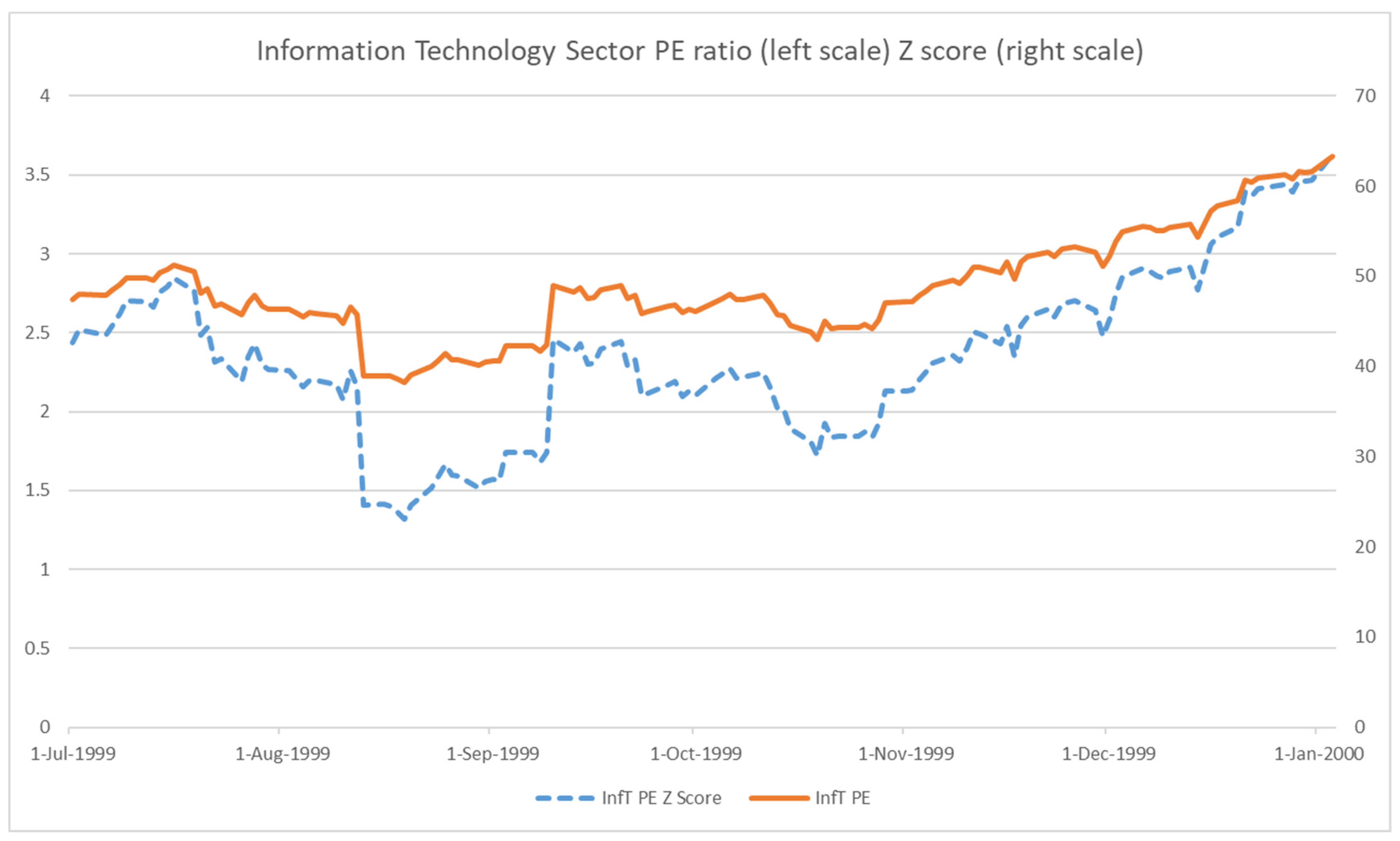
2.1. Data Transformation Methodology
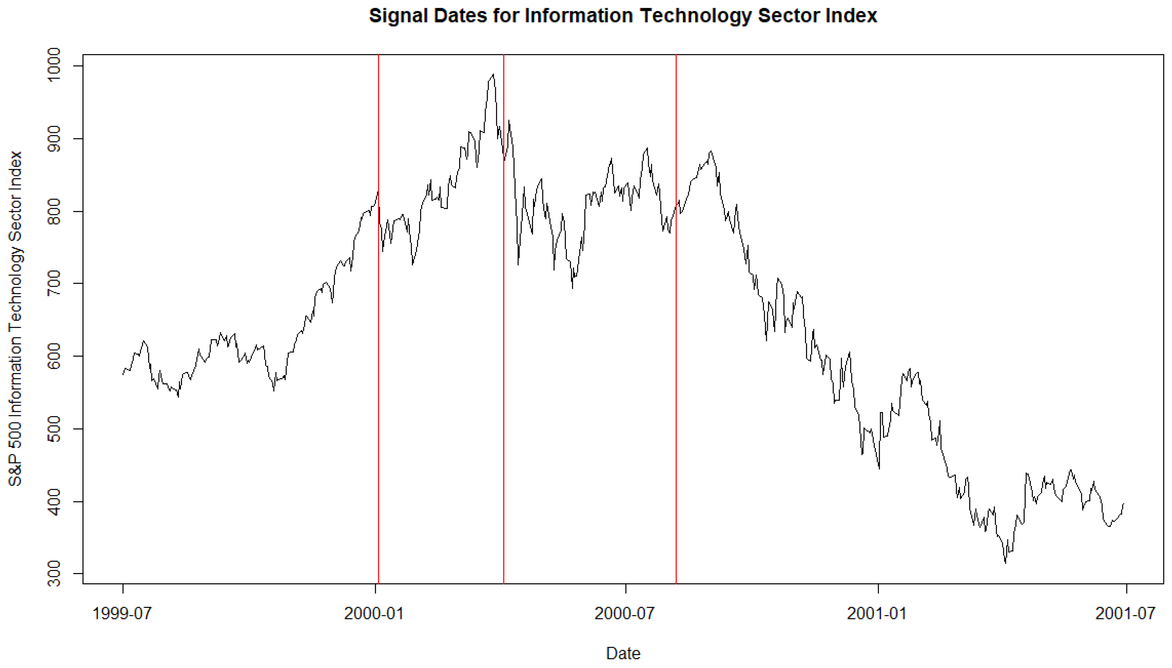
2.2. Timing Signal Construction
3. Results and Discussion
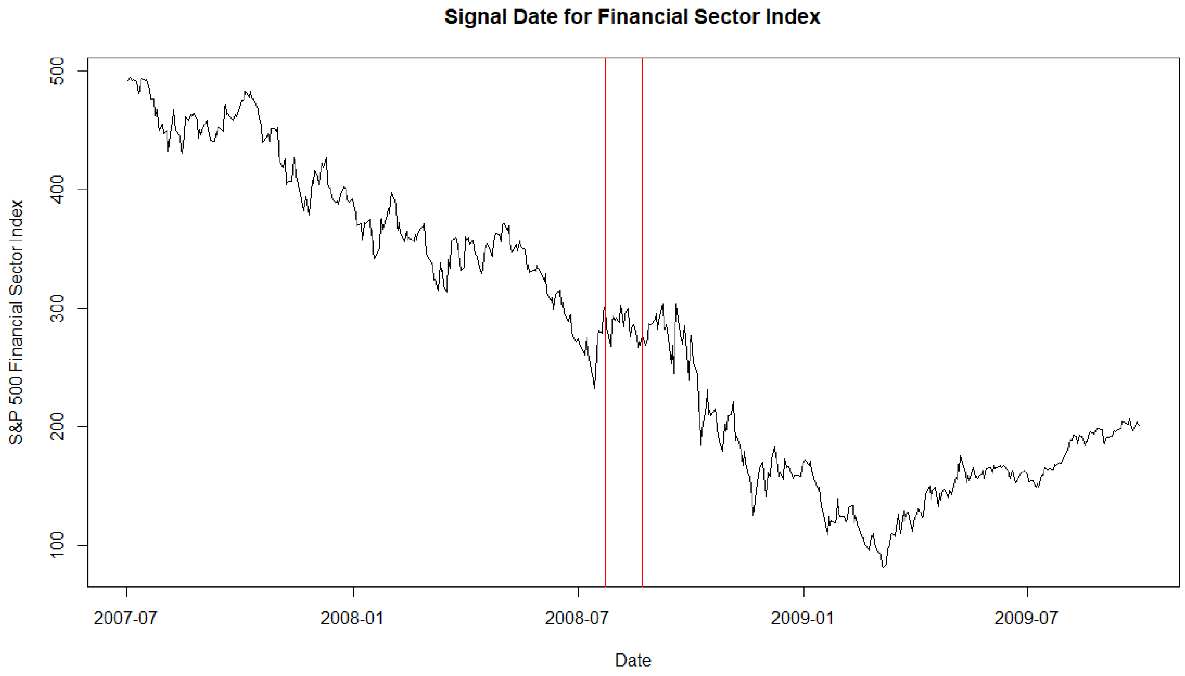
3.1. Two Major Market Crashes
3.2. Other Sectors’ Timing Signals
4. Conclusions
Author Contributions
Funding
Data Availability Statement
Acknowledgments
Conflicts of Interest
| 1 | The real estate sector is excluded from this study because it has a shorter data history than the other ten sectors. |
| 2 | According to the description provided by Bloomberg, the price is an index’s “Last Price” (i.e., Bloomberg code PX_Last). A constituent stock’s EPS (earnings per share) are based on the trailing 12-month EPS aggregate. The sector index EPS are calculated by summing up each constituent’s weight in the index multiplied by the constituent stock’s EPS. |
| 3 | Not all sectors have PE data from April 1990. However, all sectors have daily PE data starting from August 1991. |
| 4 | The empirical conditional distribution tables are available upon request. |
| 5 | For the monthly return calculation, we define a monthly return as the return during four weeks. For example, the first monthly return is from 5 January 2000 to 1 February 2000. |
| 6 | The discussion of various option implementations and the cost of downside risk hedging will be a separate topic beyond the scope of this study. This is because many possible hedging implementations depend on investors’ risk management objectives and policies. We gathered the put option premium from the Bloomberg terminal to achieve a sense of the hedging cost. On the signal dates, the six-month premiums of at-the-money put options average about 7% of the underlying sector index value. |
| 7 | Assuming the manager can hold sector index options in his/her strategy. |
| 8 | It is very rare for z-score to be bigger than 2.5. |
| 9 | The result is the same as the first signal date in Table 4. |
| 10 | The detailed results of this analysis are available upon request. |
References
- Aboura, Sofiane. 2014. When the US stock market becomes extreme? Risks 2: 211–25. [Google Scholar] [CrossRef]
- Abreu, Dilip, and Markus K. Brunnermeier. 2003. Bubbles and crashes. Econometrica 71: 173–204. [Google Scholar] [CrossRef]
- Ausloos, Marcel, Kristinka Ivanova, and Nicolas Vandewalle. 2002. Crashes: Symptoms, diagnoses and remedies. In Empirical Science of Financial Fluctuations. Tokyo: Springer, pp. 62–76. [Google Scholar]
- Berge, Klaus, Giorgio Consigli, and William T. Ziemba. 2008. The predictive ability of the bond-stock earnings yield differential model. The Journal of Portfolio Management 2008: 63–80. [Google Scholar] [CrossRef]
- Boubaker, Sabri, Zhenya Liu, Tianqing Sui, and Ling Zhai. 2022. The mirror of history: How to statistically identify stock market bubble bursts. Journal of Economic Behavior & Organization 204: 128–47. [Google Scholar]
- Cajueiro, Daniel O., Benjamin M. Tabak, and Filipe K. Werneck. 2009. Can we predict crashes? The case of the Brazilian stock market. Physica A: Statistical Mechanics and its Applications 388: 1603–9. [Google Scholar] [CrossRef]
- da Silva, Paulo Pereira. 2022. Crash risk and ESG disclosure. Borsa Istanbul Review 22: 794–811. [Google Scholar] [CrossRef]
- Deng, Shangkun, Yingke Zhu, Shuangyang Duan, Zhe Fu, and Zonghua Liu. 2022. Stock Price Crash Warning in the Chinese Security Market Using a Machine Learning-Based Method and Financial Indicators. Systems 10: 108. [Google Scholar] [CrossRef]
- Dichtl, Hubert, Wolfgang Drobetz, and Tizian Otto. 2023. Forecasting Stock Market Crashes via Machine Learning. Journal of Financial Stability 65: 101099. [Google Scholar] [CrossRef]
- Dolvin, Steven D. 2014. The Efficacy of Trading Based on Moving Average Indicators: An Extension. The Journal of Wealth Management 17: 52–57. [Google Scholar] [CrossRef]
- Farago, Adam, and Roméo Tédongap. 2018. Downside risks and the cross-section of asset returns. Journal of Financial Economics 129: 69–86. [Google Scholar] [CrossRef]
- Focardi, Sergio M., and Frank J. Fabozzi. 2014. Can We Predict Stock Market Crashes? The Journal of Portfolio Management 40: 183–95. [Google Scholar] [CrossRef]
- Fu, Junhui, Xiang Wu, Yufang Liu, and Rongda Chen. 2021. Firm-specific investor sentiment and stock price crash risk. Finance Research Letters 38: 101442. [Google Scholar] [CrossRef]
- Galsband, Victoria. 2012. Downside risk of international stock returns. Journal of Banking & Finance 36: 2379–88. [Google Scholar]
- Guan, Chong, Wenting Liu, and Jack Yu-Chao Cheng. 2022. Using social media to predict the stock market crash and rebound amid the pandemic: The digital ‘haves’ and ‘have-mores’. Annals of Data Science 9: 5–31. [Google Scholar] [CrossRef]
- Guerron-Quintana, Pablo A., Tomohiro Hirano, and Ryo Jinnai. 2023. Bubbles, crashes, and economic growth: Theory and evidence. American Economic Journal: Macroeconomics 15: 333–71. [Google Scholar] [CrossRef]
- Hull, John C. 2018. Options Futures and Other Derivatives, 10th ed. New York: Pearson Education. [Google Scholar]
- Jarrow, Robert. 2012. Detecting asset price bubbles. The Journal of Derivatives 20: 30–34. [Google Scholar] [CrossRef]
- Leiss, Matthias, Heinrich H. Nax, and Didier Sornette. 2015. Super-exponential growth expectations and the global financial crisis. Journal of Economic Dynamics and Control 55: 1–13. [Google Scholar] [CrossRef]
- Lleo, Sebastien, and William T. Ziemba. 2012. Stock market crashes in 2007–2009: Were we able to predict them? Quantitative Finance 12: 1161–87. [Google Scholar] [CrossRef]
- Lleo, Sebastien, and William T. Ziemba. 2015. Some historical perspectives on the bond-stock earnings yield model for crash prediction around the world. International Journal of Forecasting 31: 399–425. [Google Scholar] [CrossRef]
- Lleo, Sebastien, and William T. Ziemba. 2017. Does the bond-stock earnings yield differential model predict equity market corrections better than high P/E models? Financial Markets, Institutions & Instruments 26: 61–123. [Google Scholar]
- Lleo, Sebastien, and William T. Ziemba. 2019. Can Warren Buffett forecast equity market corrections? The European Journal of Finance 25: 369–93. [Google Scholar] [CrossRef]
- Mercik, Aleksander R. 2023. Is tail risk priced in the cross-section of international stock index returns? Modern Finance 1: 17–29. [Google Scholar] [CrossRef]
- Molina-Muñoz, Jesús, Andrés Mora-Valencia, and Javier Perote. 2020. Market-crash forecasting based on the dynamics of the alpha-stable distribution. Physica A: Statistical Mechanics and Its Applications 557: 124876. [Google Scholar] [CrossRef]
- Munoz Torrecillas, Maria Jose, Rossitsa Yalamova, and Bill McKelvey. 2016. Identifying the Transition from Efficient-Market to Herding Behavior: Using a Method from Econophysics. Journal of Behavioral Finance 17: 157–82. [Google Scholar] [CrossRef]
- Neely, Christopher J., David E. Rapach, Jun Tu, and Guofu Zhou. 2014. Forecasting the equity risk premium: The role of technical indicators. Management Science 60: 1772–91. [Google Scholar] [CrossRef]
- Rousseeuw, Peter J., and Mia Hubert. 2011. Robust statistics for outlier detection. Wiley Interdisciplinary Reviews: Data mining and Knowledge Discovery 1: 73–79. [Google Scholar] [CrossRef]
- Rousseeuw, Peter J., and Mia Hubert. 2018. Anomaly detection by robust statistics. Wiley Interdisciplinary Reviews: Data Mining and Knowledge Discovery 8: e1236. [Google Scholar] [CrossRef]
- Smith, C. Michael. 2017. Trading moving average crossovers: Further testing of risk-adjusted and after-tax returns. The Journal of Wealth Management 20: 94–100. [Google Scholar] [CrossRef]
- Sornette, Didier. 2009. Why Stock Markets Crash: Critical Events in Complex Financial Systems. Princeton: Princeton University Press. [Google Scholar]
- Sul, Hong Kee, Alan R. Dennis, and Lingyao Yuan. 2017. Trading on twitter: Using social media sentiment to predict stock returns. Decision Sciences 48: 454–88. [Google Scholar] [CrossRef]
- Tran, Kim Long, Hoang Anh Le, Cap Phu Lieu, and Duc Trung Nguyen. 2023. Machine Learning to Forecast Financial Bubbles in Stock Markets: Evidence from Vietnam. International Journal of Financial Studies 11: 133. [Google Scholar] [CrossRef]
- Tsakonas, Stefanos, Michael Hanias, Lykourgos Magafas, and Loukas Zachilas. 2022. Application of the moving Lyapunov exponent to the S&P 500 index to predict major declines. Journal of Risk 24. [Google Scholar] [CrossRef]
- Whitehouse, Emily J., David I. Harvey, and Stephen J. Leybourne. 2023. Real-Time Monitoring of Bubbles and Crashes. Oxford Bulletin of Economics and Statistics 85: 482–513. [Google Scholar] [CrossRef]
- Xiong, James X., Thomas M. Idzorek, and Roger G. Ibbotson. 2016. The economic value of forecasting left-tail risk. The Journal of Portfolio Management 42: 114–23. [Google Scholar] [CrossRef]
- Xu, Yahua, Jun Xiao, and Liguo Zhang. 2020. Global predictive power of the upside and downside variances of the US equity market. Economic Modelling 93: 605–19. [Google Scholar] [CrossRef]
- Yousaf, Imran, and Arshad Hassan. 2019. Linkages between crude oil and emerging Asian stock markets: New evidence from the Chinese stock market crash. Finance Research Letters 31. [Google Scholar] [CrossRef]


| Enrs | Matr | Indu | ConD | ConS | Hlth | Finl | InfT | Tels | Util | |
|---|---|---|---|---|---|---|---|---|---|---|
| Enrs | 1.000 | 0.454 | 0.322 | 0.546 | 0.238 | 0.182 | 0.373 | −0.051 | 0.345 | 0.353 |
| Matr | 0.454 | 1.000 | 0.339 | 0.337 | 0.198 | 0.202 | 0.418 | −0.103 | 0.267 | 0.445 |
| Indu | 0.322 | 0.339 | 1.000 | 0.602 | 0.481 | 0.093 | 0.594 | −0.020 | 0.255 | 0.455 |
| ConD | 0.546 | 0.337 | 0.602 | 1.000 | 0.525 | 0.351 | 0.592 | −0.060 | 0.409 | 0.440 |
| ConS | 0.238 | 0.198 | 0.481 | 0.525 | 1.000 | 0.665 | 0.552 | −0.125 | 0.176 | 0.437 |
| Hlth | 0.182 | 0.202 | 0.093 | 0.351 | 0.665 | 1.000 | 0.267 | 0.053 | −0.006 | 0.276 |
| Finl | 0.373 | 0.418 | 0.594 | 0.592 | 0.552 | 0.267 | 1.000 | −0.058 | 0.452 | 0.610 |
| InfT | −0.051 | −0.103 | −0.020 | −0.060 | −0.125 | 0.053 | −0.058 | 1.000 | 0.087 | −0.134 |
| Tels | 0.345 | 0.267 | 0.255 | 0.409 | 0.176 | −0.006 | 0.452 | 0.087 | 1.000 | 0.169 |
| Util | 0.353 | 0.445 | 0.455 | 0.440 | 0.437 | 0.276 | 0.610 | −0.134 | 0.169 | 1.000 |
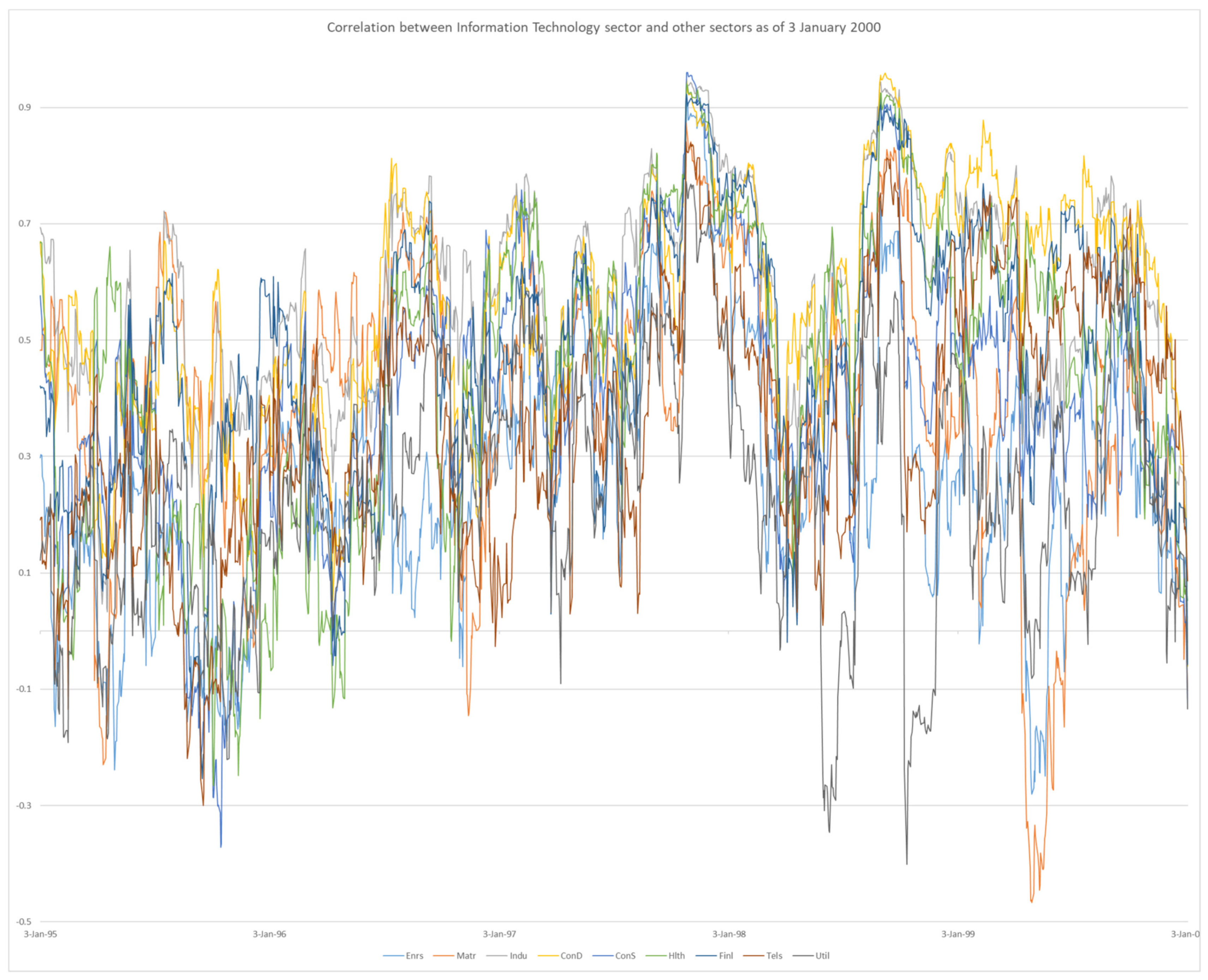
| Date | Enrs | Matr | Indu | ConD | ConS | Hlth | Finl | InfT | Tels | Util |
|---|---|---|---|---|---|---|---|---|---|---|
| 3 January 1995 | 0.298 | 0.482 | 0.694 | 0.669 | 0.577 | 0.667 | 0.421 | 1.000 | 0.191 | 0.122 |
| 4 January 1995 | 0.303 | 0.483 | 0.691 | 0.650 | 0.562 | 0.669 | 0.418 | 1.000 | 0.195 | 0.133 |
| 5 January 1995 | 0.302 | 0.482 | 0.683 | 0.640 | 0.536 | 0.667 | 0.419 | 1.000 | 0.195 | 0.143 |
| 6 January 1995 | 0.265 | 0.515 | 0.684 | 0.616 | 0.510 | 0.599 | 0.419 | 1.000 | 0.115 | 0.154 |
| : | : | : | : | : | : | : | : | : | : | : |
| : | : | : | : | : | : | : | : | : | : | : |
| : | : | : | : | : | : | : | : | : | : | : |
| 27 December 1999 | 0.122 | 0.045 | 0.270 | 0.286 | 0.049 | 0.057 | 0.211 | 1.000 | 0.307 | 0.130 |
| 28 December 1999 | 0.088 | −0.049 | 0.267 | 0.260 | 0.057 | 0.090 | 0.187 | 1.000 | 0.210 | 0.118 |
| 29 December 1999 | 0.109 | −0.009 | 0.259 | 0.219 | 0.033 | 0.070 | 0.211 | 1.000 | 0.175 | 0.099 |
| 30 December 1999 | 0.127 | 0.025 | 0.266 | 0.212 | 0.015 | 0.063 | 0.195 | 1.000 | 0.179 | 0.076 |
| 31 December 1999 | 0.113 | 0.005 | 0.257 | 0.187 | 0.016 | 0.076 | 0.193 | 1.000 | 0.162 | 0.077 |
| 3 January 2000 | −0.051 | −0.103 | −0.020 | −0.060 | −0.125 | 0.053 | −0.058 | 1.000 | 0.087 | −0.134 |
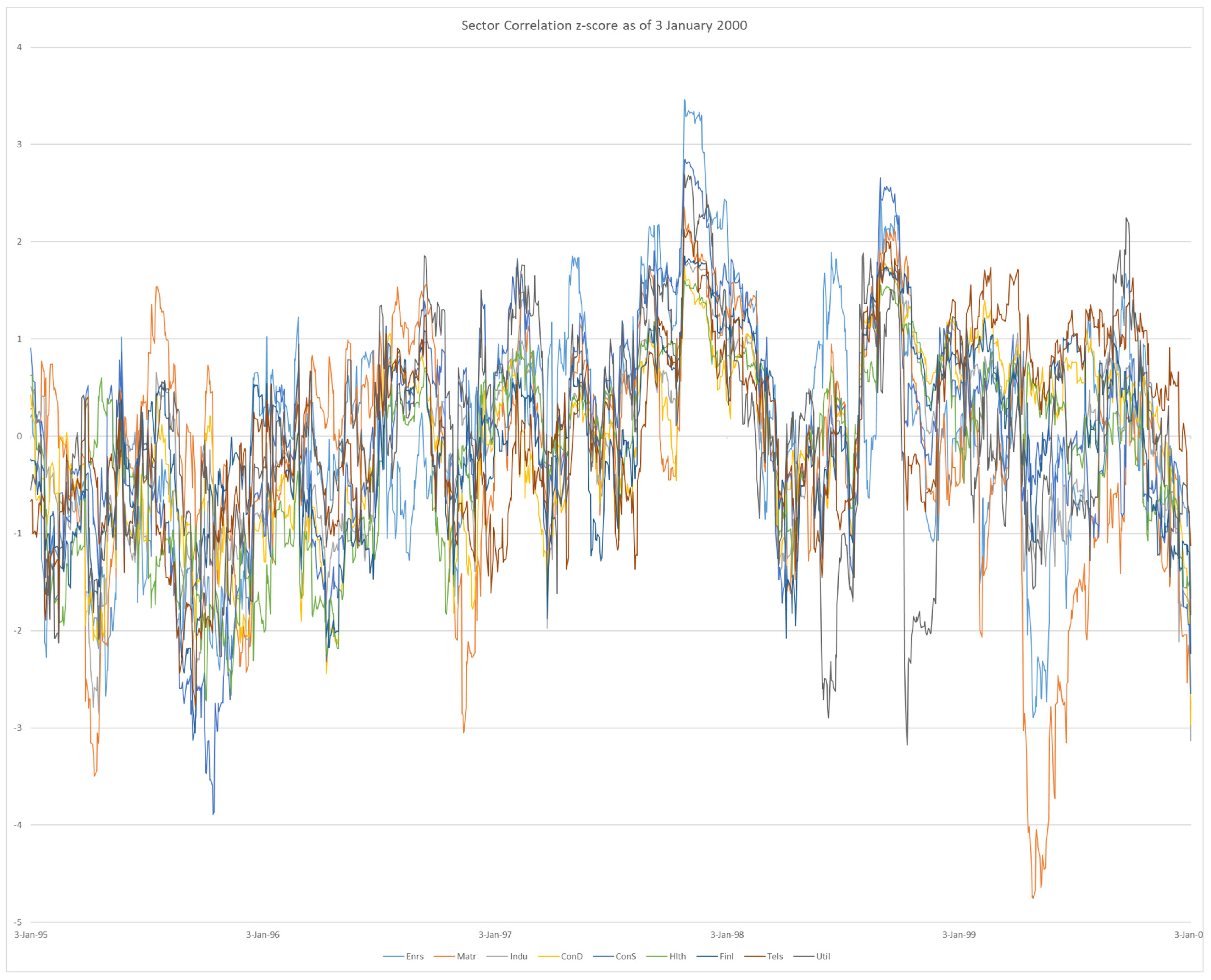
| Date | Enrs | Matr | Indu | ConD | ConS | Hlth | Finl | InfT | Tels | Util |
|---|---|---|---|---|---|---|---|---|---|---|
| 3 January 1995 | 0.192 | 0.279 | 0.511 | 0.428 | 0.904 | 0.625 | −0.240 | −0.673 | −0.554 | |
| 4 January 1995 | 0.218 | 0.285 | 0.499 | 0.336 | 0.828 | 0.629 | −0.254 | −0.656 | −0.501 | |
| 5 January 1995 | 0.216 | 0.280 | 0.455 | 0.291 | 0.700 | 0.624 | −0.249 | −0.656 | −0.450 | |
| 6 January 1995 | 0.019 | 0.455 | 0.462 | 0.177 | 0.568 | 0.380 | −0.251 | −1.000 | −0.391 | |
| : | : | : | : | : | : | : | : | : | : | |
| : | : | : | : | : | : | : | : | : | : | |
| : | : | : | : | : | : | : | : | : | : | |
| 27 December 1999 | −0.746 | −2.039 | −1.648 | −1.357 | −1.765 | −1.562 | −1.115 | −0.173 | −0.514 | |
| 28 December 1999 | −0.926 | −2.536 | −1.666 | −1.475 | −1.727 | −1.445 | −1.216 | −0.590 | −0.572 | |
| 29 December 1999 | −0.816 | −2.328 | −1.706 | −1.669 | −1.844 | −1.517 | −1.118 | −0.742 | −0.668 | |
| 30 December 1999 | −0.718 | −2.147 | −1.672 | −1.698 | −1.940 | −1.541 | −1.183 | −0.725 | −0.783 | |
| 31 December 1999 | −0.792 | −2.249 | −1.718 | −1.818 | −1.930 | −1.497 | −1.192 | −0.799 | −0.778 | |
| 3 January 2000 | −1.667 | −2.824 | −3.130 | −2.964 | −2.646 | −1.579 | −2.236 | −1.124 | −1.834 |
| Signal Date | 3 January 2000 | 3 April 2000 | 7 August 2000 |
|---|---|---|---|
| PE z-score | 3.63 | 3.50 | 2.56 |
| Count | 5 | 4 | 4 |
| 1st month return (%) | −2.36 | −6.41 | 6.09 |
| 2nd month return (%) | 10.60 | −6.30 | −19.57 |
| 3rd month return (%) | 14.00 | 7.53 | −2.54 |
| 4th month return (%) | −15.32 | 2.00 | −15.80 |
| 5th month return (%) | −15.03 | 1.10 | −13.02 |
| 6th month return (%) | 24.65 | −5.12 | 17.26 |
| Pseudo-pvalue [95% Confidence Interval] | 0.0149 [0.0124, 0.0175] | 0.0647 [0.0594, 0.0701] | 0.0072 [0.0054, 0.0091] |
| Energy | −1.67 | −2.46 | −2.03 |
| Materials | −2.82 | −2.77 | −2.16 |
| Industrials | −3.13 | −1.42 | −0.49 |
| Consumer Discretionary | −2.96 | −2.37 | −0.65 |
| Consumer Staples | −2.65 | −3.25 | −2.81 |
| Health Care | −1.58 | −1.77 | −2.67 |
| Financials | −2.24 | −1.43 | −0.22 |
| Information Technology | |||
| Communication Services | −1.12 | −0.01 | 0.15 |
| Utilities | −1.83 | −0.82 | −0.75 |
| Signal Date | 23 July 2008 | 12 April 2021 |
|---|---|---|
| PE z-score | 2.54 | 2.50 |
| Count | 4 | 5 |
| 1st month return (%) | −4.35 | 6.14 |
| 2nd month return (%) | 2.00 | 2.81 |
| 3rd month return (%) | −21.55 | −4.27 |
| 4th month return (%) | −15.98 | 1.54 |
| 5th month return (%) | −11.17 | 4.05 |
| 6th month return (%) | 2.27 | −0.32 |
| pseudo-pvalue [95% Confidence Interval] | 0.0058 [0.0043, 0.0075] | 0.2175 [0.2087, 0.2265] |
| Energy | −2.63 | −0.07 |
| Materials | −2.35 | −0.04 |
| Industrials | −0.04 | 0.24 |
| Consumer Discretionary | 0.70 | −4.97 |
| Consumer Staples | −0.75 | −2.07 |
| Health Care | −0.77 | −2.03 |
| Financials | ||
| Information Technology | −0.06 | −3.30 |
| Communication Services | −2.13 | −2.55 |
| Utilities | −3.77 | −1.77 |
| Signal Date | 11 June 1998 | 9 October 1998 | 16 January 2020 |
|---|---|---|---|
| PE z-score | 2.56 | 2.52 | 2.51 |
| Count | 7 | 5 | 4 |
| 1st month return (%) | −1.21 | −1.14 | 5.40 |
| 2nd month return (%) | −4.26 | 1.36 | −18.14 |
| 3rd month return (%) | 0.73 | 1.03 | 6.57 |
| 4th month return (%) | 12.07 | −4.38 | −7.70 |
| 5th month return (%) | −3.88 | −3.81 | 9.04 |
| 6th month return (%) | 3.08 | 1.64 | −4.65 |
| Pseudo-pvalue [95% Confidence Interval] | 0.1207 [0.1138, 0.1277] | 0.1214 [0.1144, 0.1284] | 0.0074 [0.0056, 0.0093] |
| Energy | −2.62 | −0.24 | 2.87 |
| Materials | −2.33 | −1.96 | −0.52 |
| Industrials | −2.78 | −3.53 | −2.71 |
| Consumer Discretionary | −1.82 | −3.60 | −2.31 |
| Consumer Staples | −2.67 | −1.09 | 0.46 |
| Health Care | −3.17 | −2.92 | −0.75 |
| Financials | −2.57 | −4.74 | −2.65 |
| Information Technology | −3.23 | −2.39 | −1.29 |
| Communication Services | −1.76 | 0.57 | −1.78 |
| Utilities |
| Signal Date | 19 April 1999 |
|---|---|
| PE Z-score | 3.19 |
| Count | 4 |
| 1st month return (%) | −1.99 |
| 2nd month return (%) | −5.08 |
| 3rd month return (%) | 8.46 |
| 4th month return (%) | −10.98 |
| 5th month return (%) | 11.17 |
| 6th month return (%) | −6.80 |
| Pseudo-pvalue [95% Confidence Interval] | 0.0137 [0.0113, 0.0162] |
| Energy | −2.34 |
| Materials | −2.82 |
| Industrials | −2.13 |
| Consumer Discretionary | 0.99 |
| Consumer Staples | −1.06 |
| Health Care | |
| Financials | −0.85 |
| Information Technology | 0.35 |
| Communication Services | 1.09 |
| Utilities | −2.37 |
| Signal Date | 21 April 1999 | 7 March 2000 | 14 June 2017 | 6 November 2017 |
|---|---|---|---|---|
| PE z-score | 5.03 | 3.84 | 8.10 | 4.32 |
| Count | 4 | 4 | 4 | 6 |
| 1st month return (%) | 0.82 | 2.41 | −0.31 | −1.00 |
| 2nd month return (%) | 4.26 | −0.16 | −0.96 | 6.45 |
| 3rd month return (%) | 1.50 | 9.99 | 1.10 | 1.90 |
| 4th month return (%) | 2.67 | −3.32 | 6.67 | −8.65 |
| 5th month return (%) | 0.60 | −7.74 | −0.14 | −0.79 |
| 6th month return (%) | −11.63 | 15.45 | 0.98 | 8.31 |
| Pseudo-pvalue [95% Confidence Interval] | 0.0122 [0.0099, 0.0146] | 0.1402 [0.1327, 0.1477] | 0.3100 [0.3002, 0.3200] | 0.1546 [0.1469, 0.1623] |
| Energy | ||||
| Materials | −0.13 | −2.23 | −0.28 | −2.06 |
| Industrials | −1.85 | −3.01 | −1.39 | −1.89 |
| Consumer Discretionary | −2.19 | −1.98 | −2.19 | −0.23 |
| Consumer Staples | −1.70 | −3.55 | −2.27 | −2.30 |
| Health Care | −3.37 | −2.24 | −1.73 | −2.05 |
| Financials | −1.81 | −1.82 | −0.50 | −2.08 |
| Information Technology | −2.09 | −1.88 | −2.25 | −0.92 |
| Communication Services | −2.27 | −0.80 | −0.84 | −2.08 |
| Utilities | −0.47 | 0.08 | −3.47 | −3.72 |
| Signal Date | 10 November 2020 | 12 January 2021 | 14 April 2021 | 26 January 2021 | 21 April 2021 | 25 August 2021 |
|---|---|---|---|---|---|---|
| PE z-score | 4.92 | 5.90 | 7.95 | 4.23 | 7.07 | 4.24 |
| Count | 4 | 4 | 4 | 4 | 4 | 4 |
| 1st month return (%) | 1.88 | 1.74 | −6.02 | 9.34 | 2.10 | −3.07 |
| 2nd month return (%) | 3.19 | −4.41 | 3.04 | 2.30 | −1.63 | 3.75 |
| 3rd month return (%) | 4.23 | 6.15 | 5.88 | 6.15 | 2.23 | 1.75 |
| 4th month return (%) | −6.22 | 1.08 | −0.54 | 1.34 | 2.45 | −1.91 |
| 5th month return (%) | 5.26 | −2.12 | 0.93 | 0.19 | −2.75 | 2.52 |
| 6th month return (%) | 6.66 | 4.37 | −2.50 | 0.42 | −1.12 | −5.20 |
| Pseudo-pvalue [95% Confidence Interval] | 0.0276 [0.0241, 0.0312] | 0.1296 [0.1226, 0.1369] | 0.1378 [0.1304, 0.1452] | 0.0425 [0.0382, 0.0469] | 0.2180 [0.2091, 0.2268] | 0.1151 [0.1083, 0.1220] |
| Energy | −2.03 | −1.18 | −2.16 | 0.38 | −0.60 | 0.42 |
| Materials | −2.29 | −2.51 | −1.84 | 0.58 | 0.45 | 0.54 |
| Industrials | −5.32 | −4.59 | −4.40 | |||
| Consumer Discretionary | −4.41 | −3.12 | −2.42 | |||
| Consumer Staples | −0.76 | −0.92 | −2.19 | −2.88 | −1.63 | −2.32 |
| Health Care | −0.33 | −2.52 | −1.17 | −1.61 | −1.20 | −3.20 |
| Financials | −6.74 | −4.93 | −5.82 | 0.03 | 0.50 | 0.57 |
| Information Technology | 1.11 | −0.83 | 0.13 | −4.09 | −2.42 | −2.07 |
| Communication Services | 1.37 | −0.01 | 0.32 | −2.14 | −2.04 | −0.54 |
| Utilities | −1.02 | −0.65 | −0.77 | −0.71 | −2.36 | −1.46 |
| Signal Date | 3 January 2000 |
|---|---|
| BSEYD z-score | 2.12 |
| Count | 5 |
| 1st month return (%) | −2.36 |
| 2nd month return (%) | 10.60 |
| 3rd month return (%) | 14.00 |
| 4th month return (%) | −15.32 |
| 5th month return (%) | −15.03 |
| 6th month return (%) | 24.65 |
| Pseudo-pvalue [95% Confidence Interval] | 0.0149 [0.0124, 0.0175] |
| Energy | −1.67 |
| Materials | −2.82 |
| Industrials | −3.13 |
| Consumer Discretionary | −2.96 |
| Consumer Staples | −2.65 |
| Health Care | −1.58 |
| Financials | −2.24 |
| Information Technology | |
| Communication Services | −1.12 |
| Utilities | −1.83 |
| Signal Date | 22 August 2008 |
|---|---|
| BSEYD z-score | 2.05 |
| Count | 3 |
| 1st month return (%) | 9.92 |
| 2nd month return (%) | −31.02 |
| 3rd month return (%) | −18.46 |
| 4th month return (%) | −4.39 |
| 5th month return (%) | −3.21 |
| 6th month return (%) | −15.33 |
| Pseudo-pvalue [95% Confidence Interval] | 0.0032 [0.0020, 0.0045] |
| Energy | −2.06 |
| Materials | −2.01 |
| Industrials | 0.43 |
| Consumer Discretionary | 0.54 |
| Consumer Staples | 0.03 |
| Health Care | −0.23 |
| Financials | |
| Information Technology | 0.39 |
| Communication Services | 0.25 |
| Utilities | −2.05 |
| Death Cross Analysis | Number of Signals | Average Number of Negative Monthly Returns within Six Months Period after Signal | Percentage of Significant Signal Pseudo-Pvalue |
|---|---|---|---|
| Consumer Discretionary | 17 | 2.0 | 35.3% |
| Consumer Staples | 18 | 2.0 | 22.2% |
| Energy | 17 | 2.4 | 0.0% |
| Financial | 16 | 2.6 | 56.3% |
| Health | 18 | 2.2 | 33.3% |
| Industrials | 16 | 2.4 | 25.0% |
| Information Technology | 17 | 2.6 | 29.4% |
| Materials | 19 | 2.3 | 31.6% |
| Communications | 19 | 2.4 | 15.8% |
| Utilities | 17 | 2.7 | 17.6% |
Disclaimer/Publisher’s Note: The statements, opinions and data contained in all publications are solely those of the individual author(s) and contributor(s) and not of MDPI and/or the editor(s). MDPI and/or the editor(s) disclaim responsibility for any injury to people or property resulting from any ideas, methods, instructions or products referred to in the content. |
© 2024 by the authors. Licensee MDPI, Basel, Switzerland. This article is an open access article distributed under the terms and conditions of the Creative Commons Attribution (CC BY) license (https://creativecommons.org/licenses/by/4.0/).
Share and Cite
Giannikos, C.I.; Guirguis, H.; Kakolyris, A.; Suen, T.S. When to Hedge Downside Risk? Risks 2024, 12, 42. https://doi.org/10.3390/risks12020042
Giannikos CI, Guirguis H, Kakolyris A, Suen TS. When to Hedge Downside Risk? Risks. 2024; 12(2):42. https://doi.org/10.3390/risks12020042
Chicago/Turabian StyleGiannikos, Christos I., Hany Guirguis, Andreas Kakolyris, and Tin Shan (Michael) Suen. 2024. "When to Hedge Downside Risk?" Risks 12, no. 2: 42. https://doi.org/10.3390/risks12020042