
Cancerous and Non-Cancerous Brain MRI Classification Method Based on Convolutional Neural Network and Log-Polar Transformation


 ,
,  ,
, 
 , , ,
, , ,  and
and 
Abstract
:1. Introduction
2. Related Works
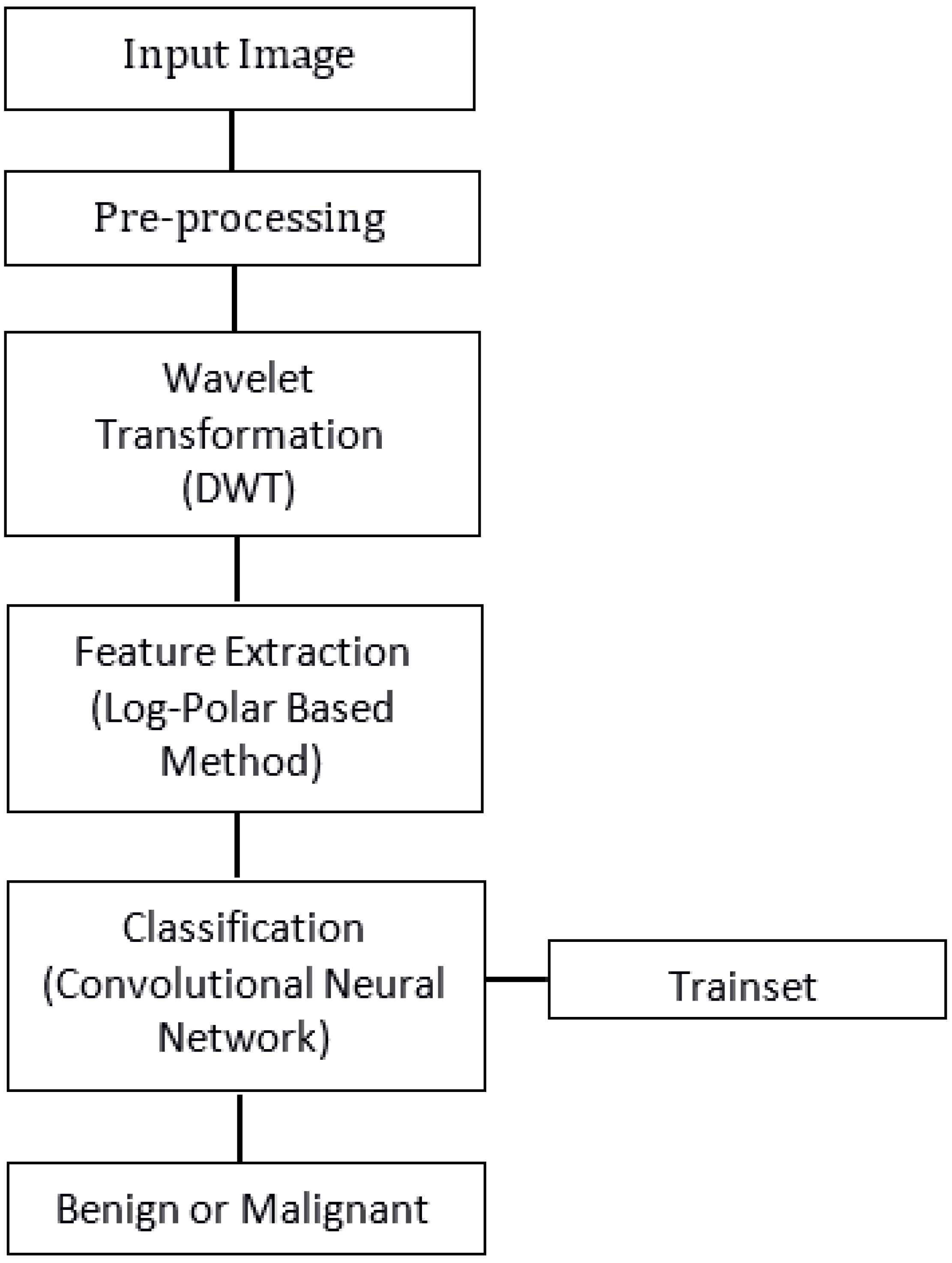
3. Proposed Method
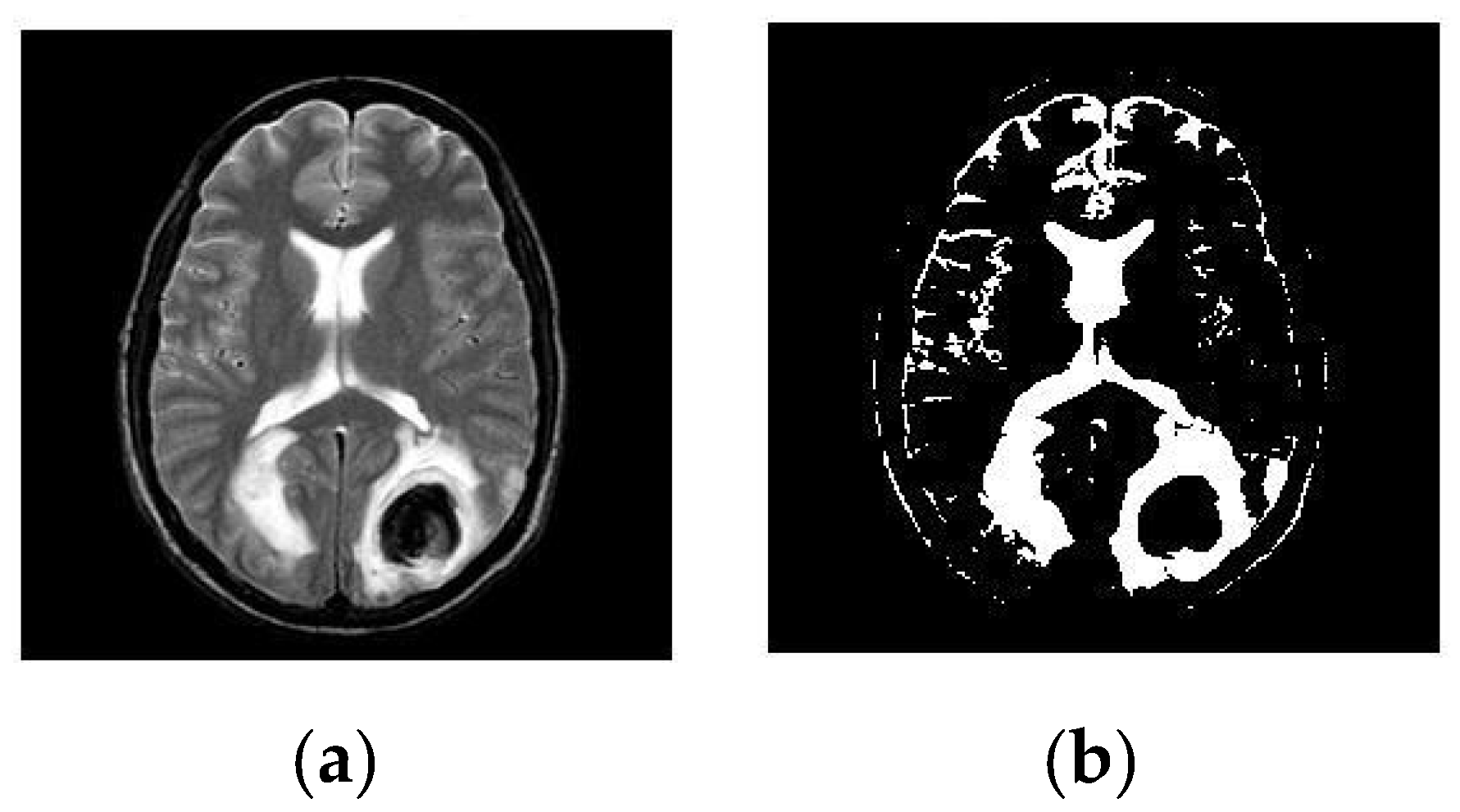
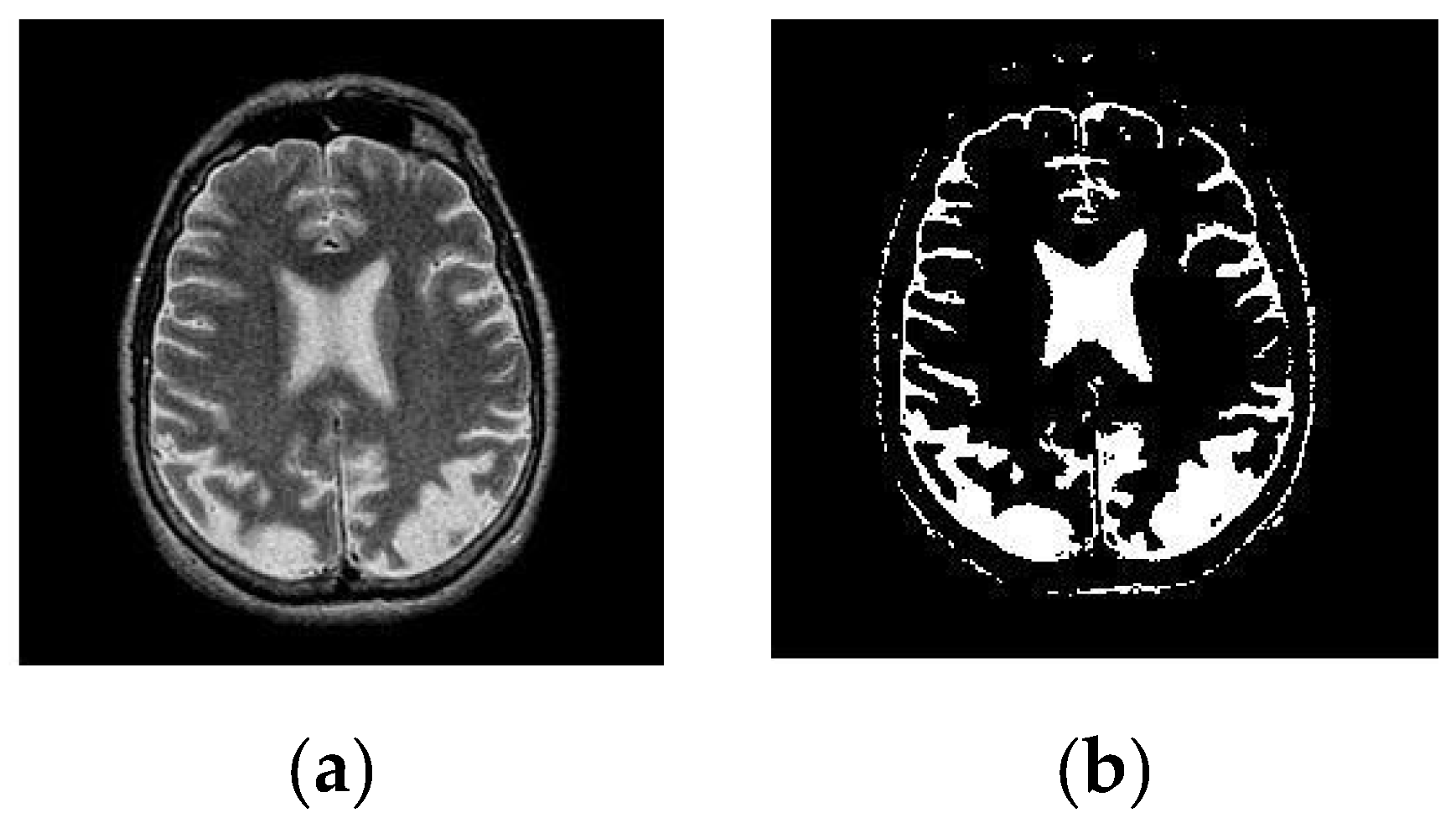
3.1. Pre-Processing
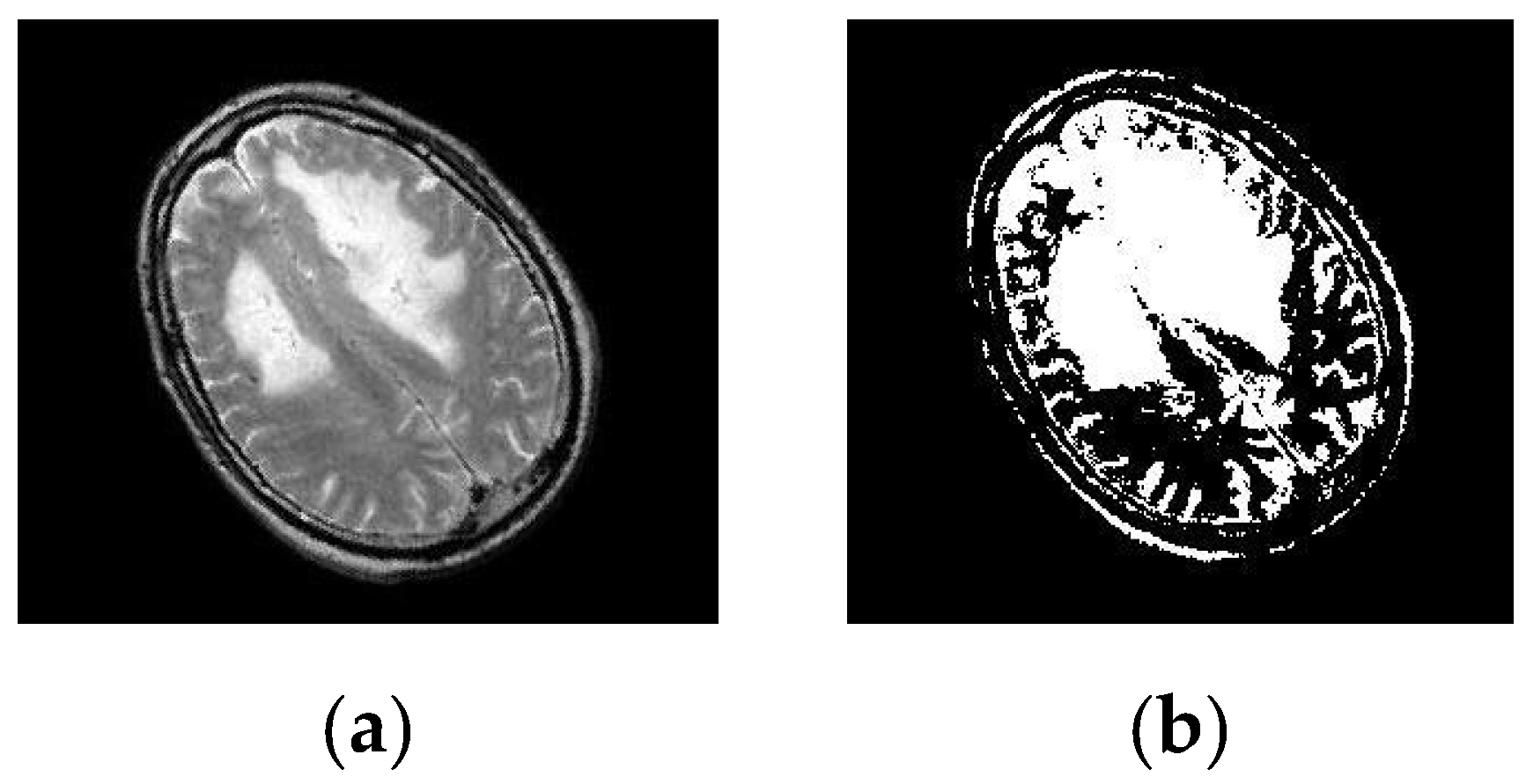
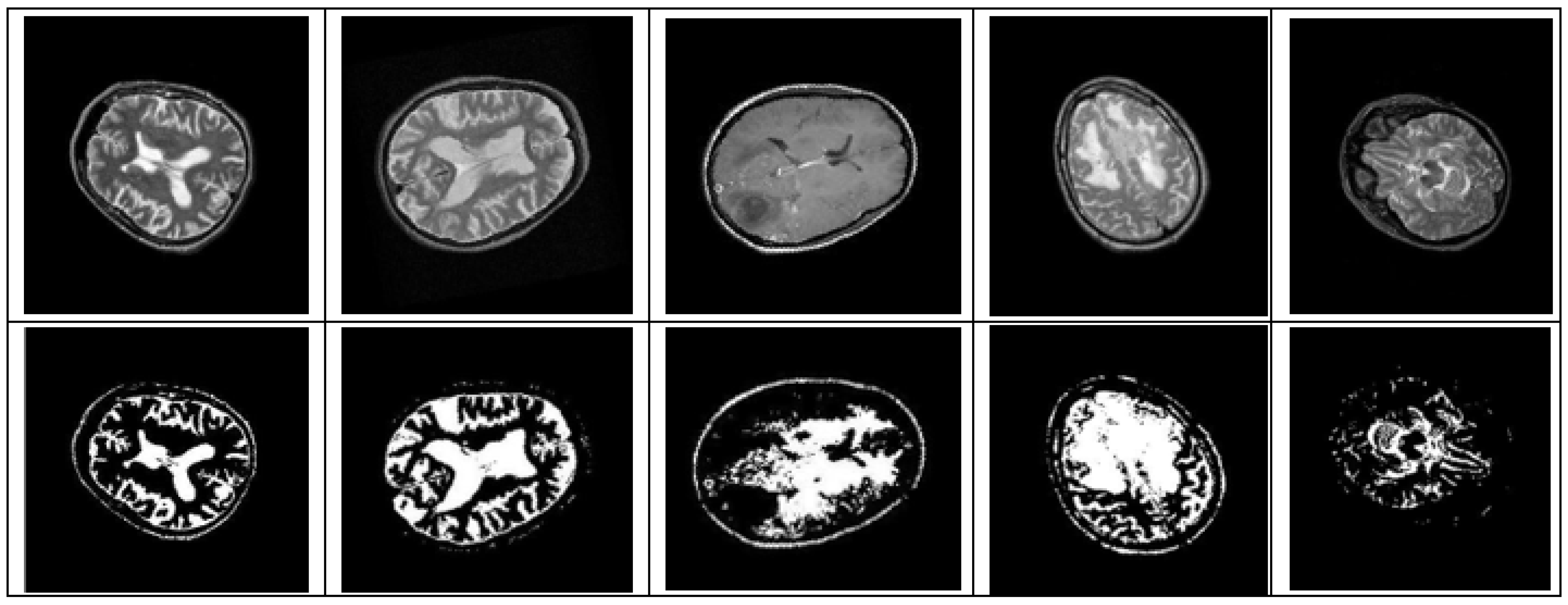
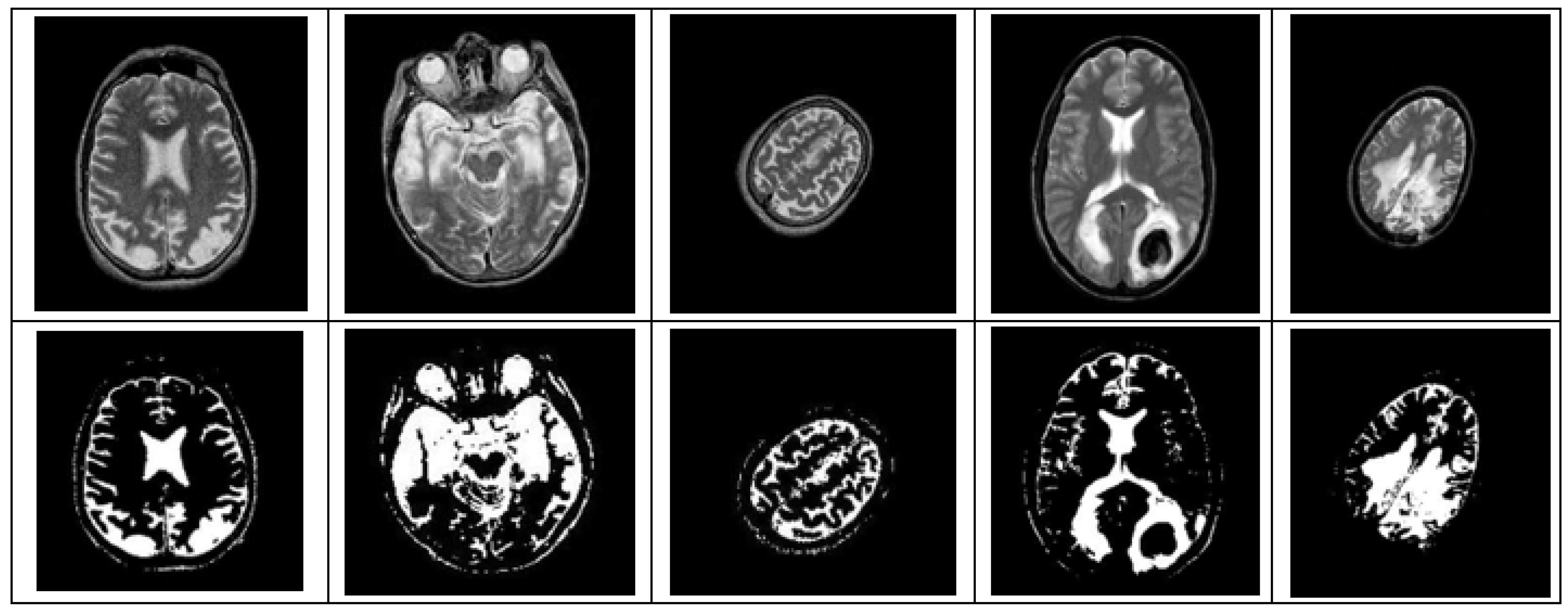
3.2. Segmentation
3.3. Feature Extraction
3.3.1. Discrete Wavelet Transform (DWT)
3.3.2. Log-Polar Transformation (LPT)
3.3.3. Independent Component Analysis (ICA)
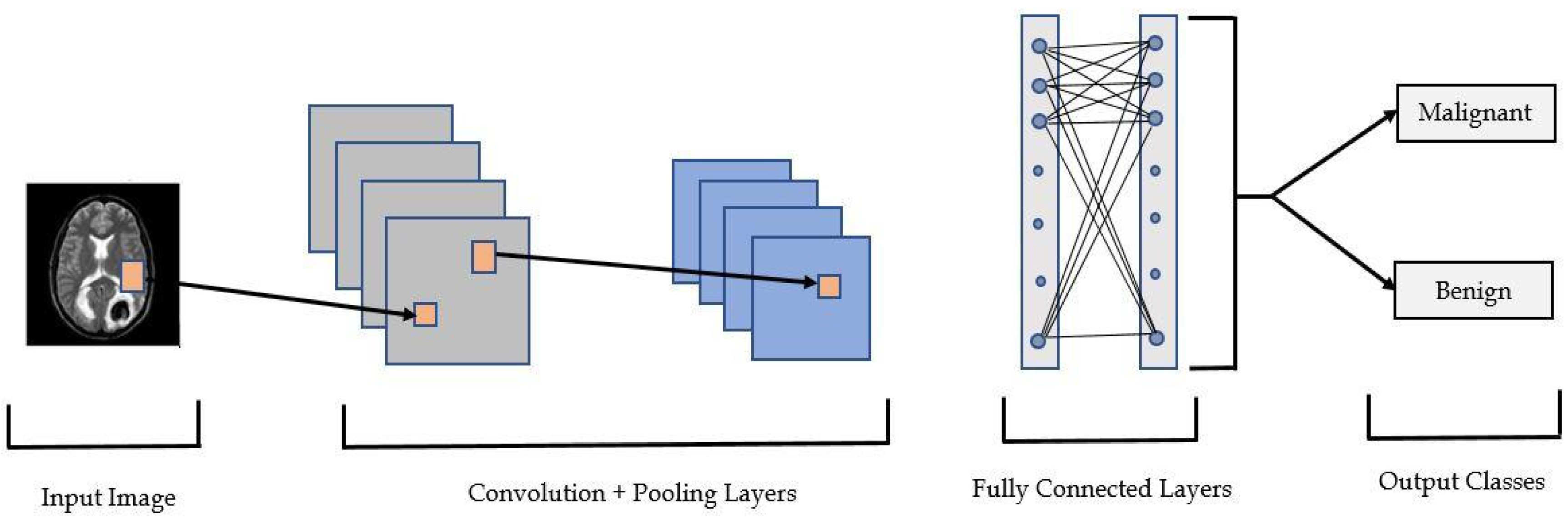
3.4. Classification
Convolutional Neural Network (CNN)
4. Experiment
4.1. Dataset Formation
4.2. Design Simulation
4.3. Simulation and Observation/Output of Simulation
5. Result Analysis
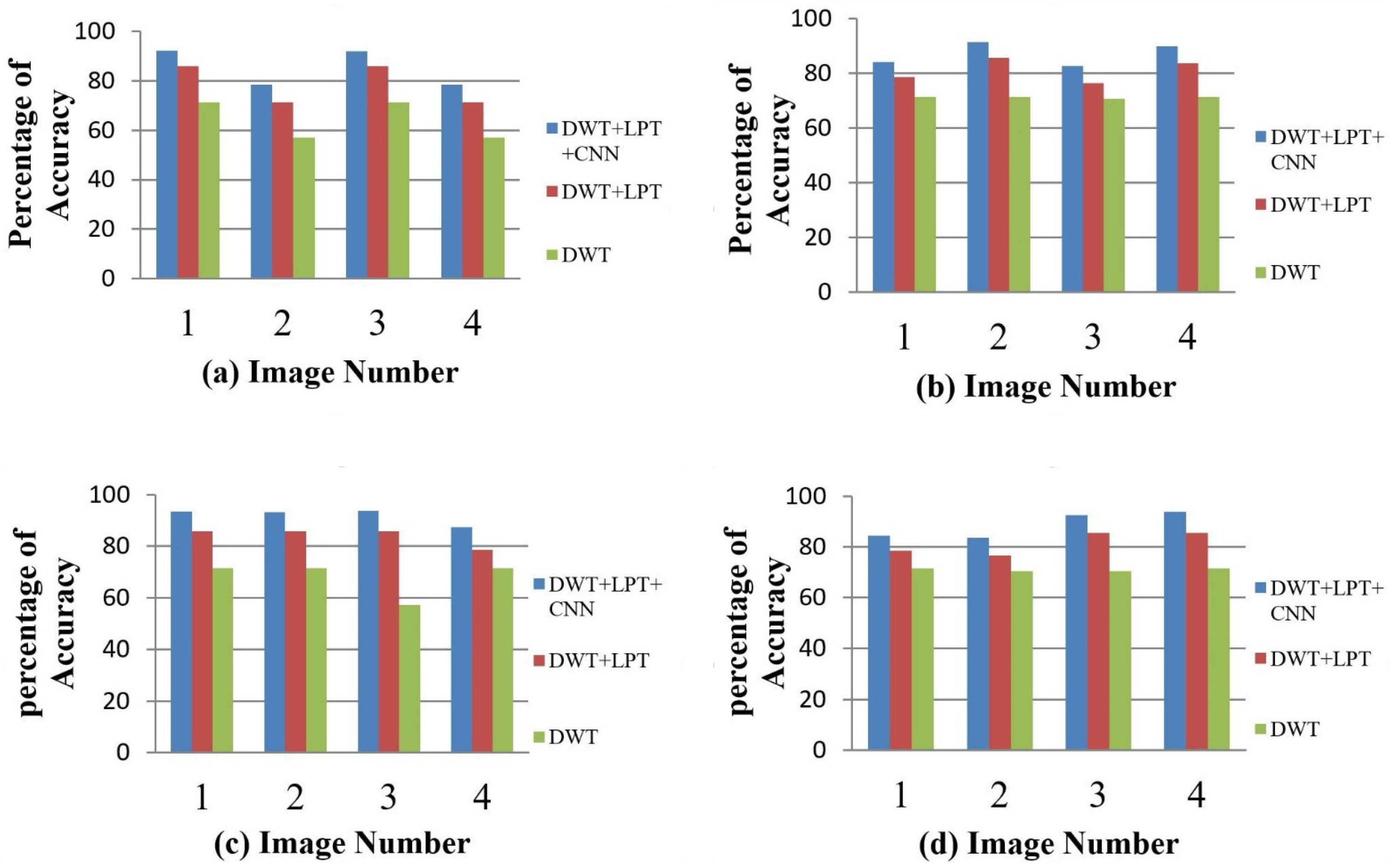
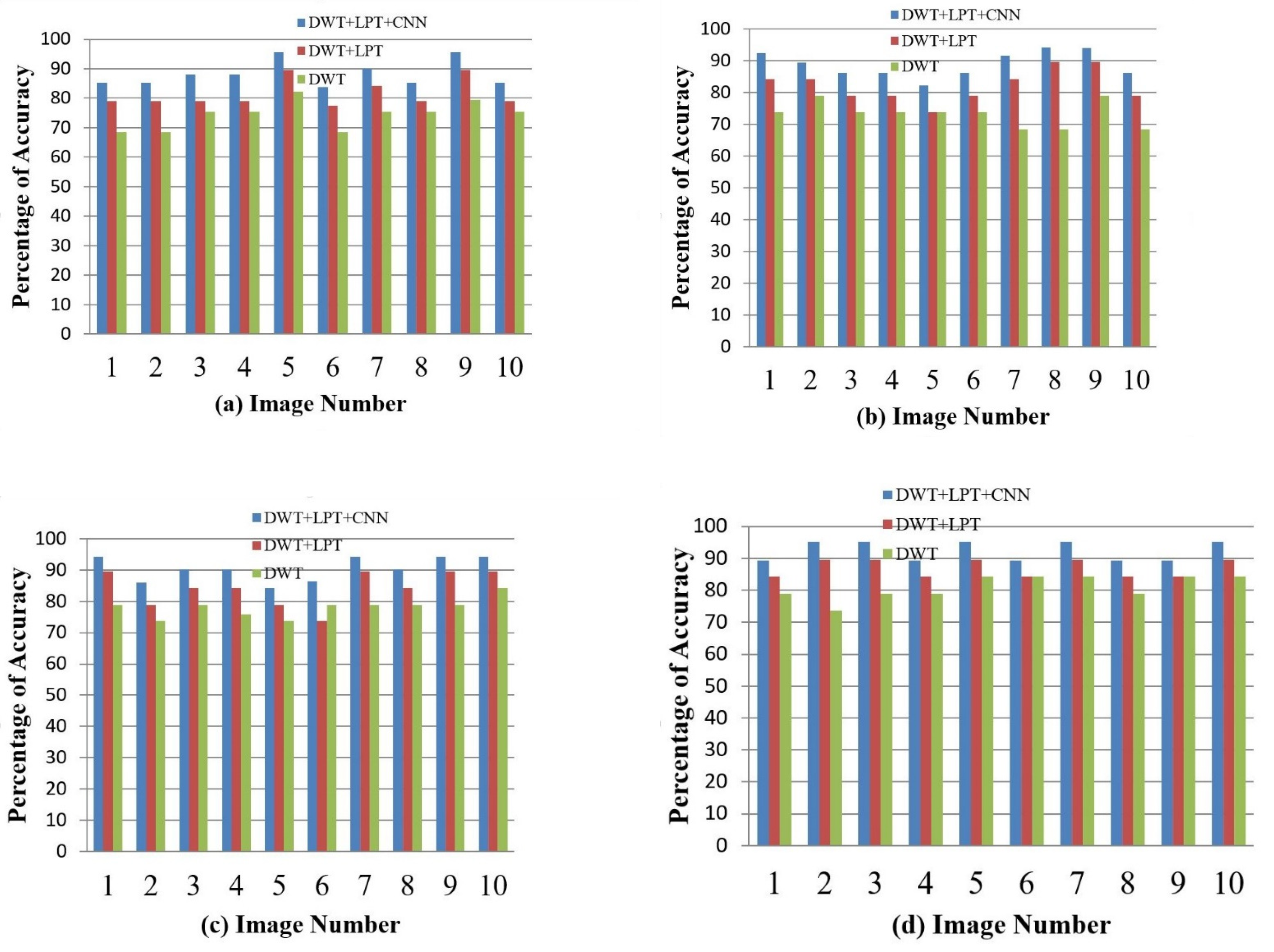
5.1. Result 1: Experiment with Distorted/Simulated MRI Image Dataset
- (a)
- Abnormality Classification for Distorted/Simulated MRI Image:
- (b)
- Tumor Classification for Distorted/Simulated MRI Image
5.2. Result 2: Experiment with T-1 Weighted MRI Image Dataset
- (a)
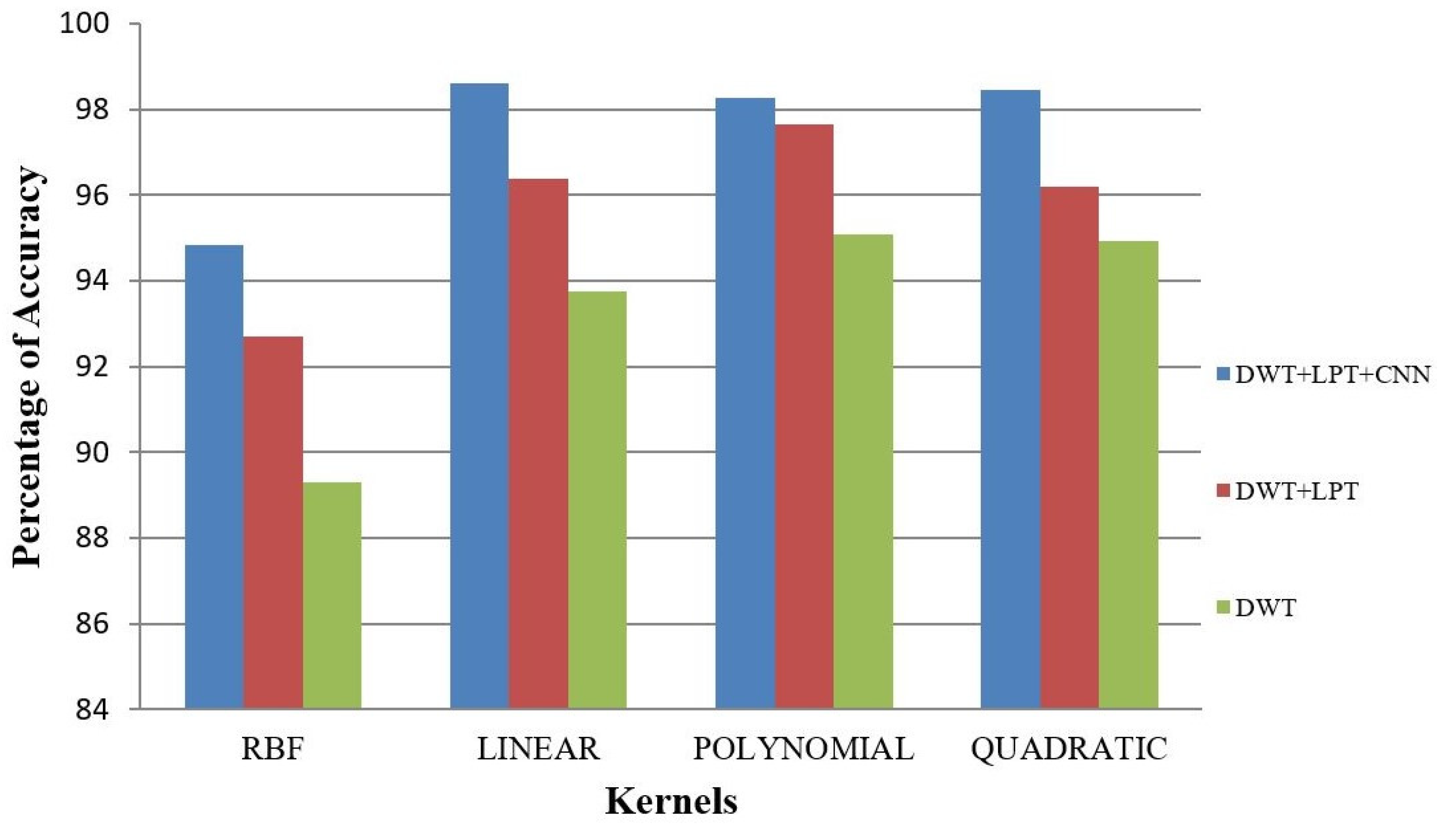
- Abnormality Classification for T-1 Weighted Images
- (b)
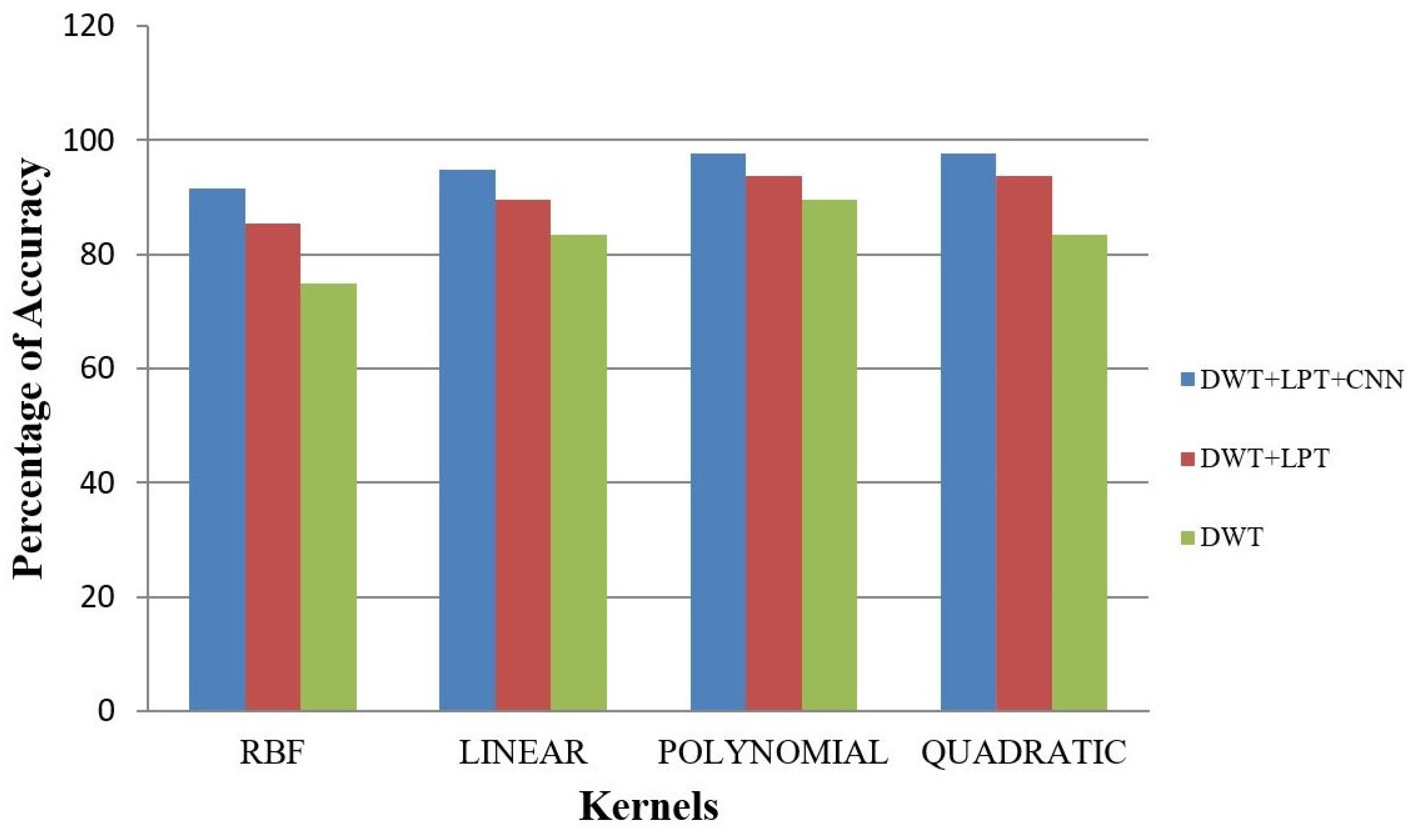
- T-1 Weighted Image Tumor Classification
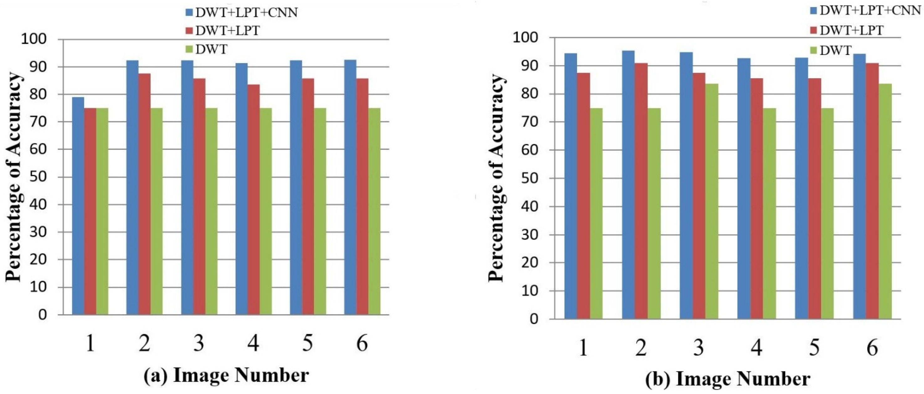
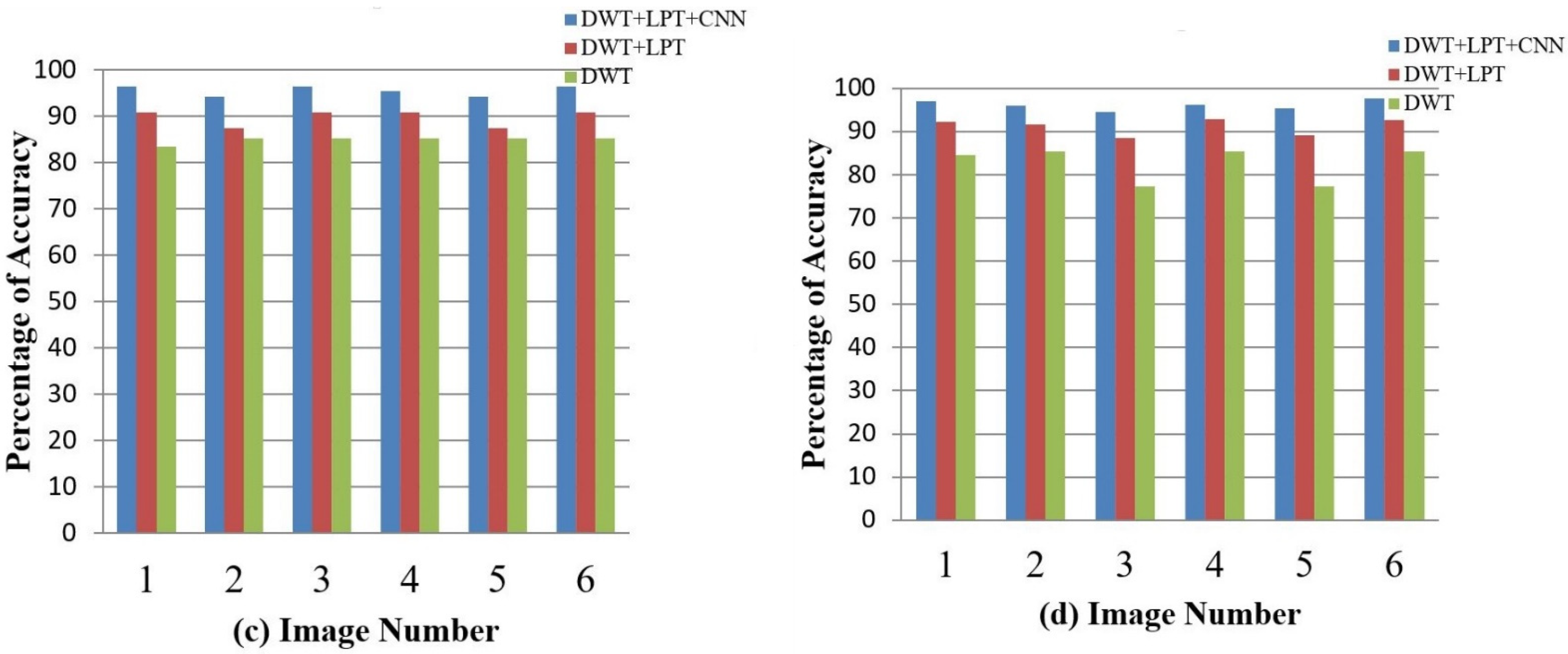
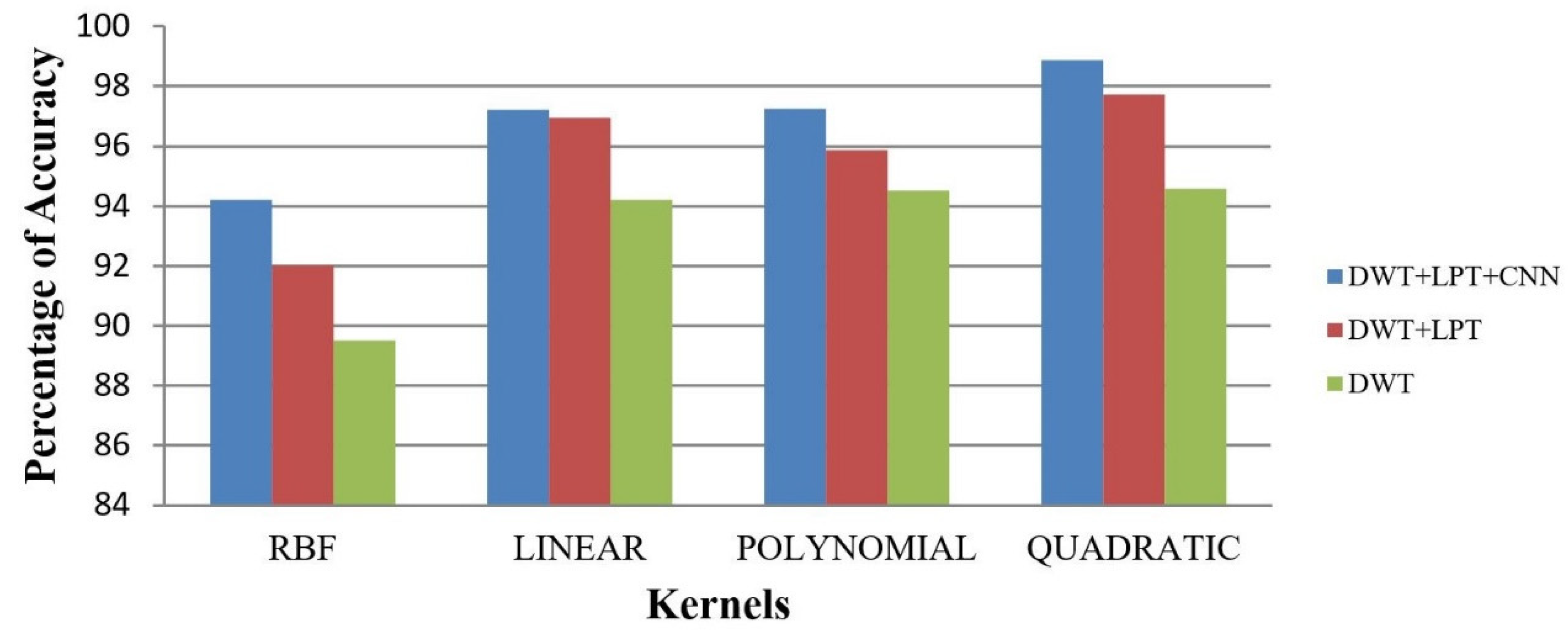
5.3. Result 3: Experiment with T-2 Weighted MRI Image Dataset
- (a)
- Classification of Abnormalities in T-2 Weighted Images
- (b)
- Tumor Classification for T-2 Weighted Images


6. Conclusions
7. Limitations
Author Contributions
Funding
Institutional Review Board Statement
Informed Consent Statement
Data Availability Statement
Acknowledgments
Conflicts of Interest
References
- Zhang, Y.; Wu, L. An MR Brain Images Classifier VIA Principal Component Analysis and Kernel Support Vector Machine. Prog. Electromagn. Res. 2012, 130, 369–388. [Google Scholar] [CrossRef]
- Jibon, F.A.; Islam, M.S.; Islam, R. Log-polar Transformation based Feature Extraction Method for Tumor Detection and Classification of brain MRI. DUET J. 2019, 5, 9–16. [Google Scholar]
- Sarhan, A.M. Detection and Classification of Brain Tumor in MRI Images Using Wavelet Transform and Convolutional Neural Network. J. Adv. Med. Med. Res. 2020, 32, 15–26. [Google Scholar] [CrossRef]
- Kharat, K.D.; Pawar, V.J.; Pardeshi, S.R. Feature Extraction and selection from MRI Images for the brain tumor classification. In Proceedings of the 2016 International Conference on Communication and Electronics Systems (ICCES), Coimbatore, India, 21–22 October 2016. [Google Scholar]
- Fayaz, M.; Torokeldiev, N.; Turdumamatov, S.; Qureshi, M.S.; Qureshi, M.B.; Gwak, J. An Efficient Methodology for Brain MRI Classification Based on DWT and Convolutional Neural Network. Sensors 2021, 22, 7480. [Google Scholar] [CrossRef] [PubMed]
- Suganaya, S.; Padmaja, S.; Suseendran, G. MRI geometric distortion for brain tumor detection and segmentation. J. Adv. Res. Dyn. Control. Syst. 2017, 9, 77–82. [Google Scholar]
- Gurusamy, R.; Subramaniam, V. A Machine Learning Approach for MRI Brain Tumor Classification. Comput. Mater. Contin. 2017, 53, 91–109. [Google Scholar]
- Bauer, S.; Wiest, R.; Nolte, L.-P.; Reyes, M. A survey of MRI-based medical image analysis for brain tumor studies. Phys. Med. Biol. 2013, 58, 1–44. [Google Scholar] [CrossRef]
- Anithadevi, D.; Perumal, K. A Hybrid Approach Based Segmentation. Signal Image Processing Int. J. (SIPIJ) 2016, 7, 21–30. [Google Scholar]
- Anjana, E.; Kaur, E.R. Review of Image Segmentation Technique. Int. J. Adv. Res. Comput. Sci. 2017, 8, 36–39. [Google Scholar]
- Zhang, Y.; Dong, Z.; Wang, S.; Ji, G.; Yang, J. Preclinical Diagnosis of Magnetic Resonance (MR) Brain Images via Discrete Wavelet Packet Transform with Tsallis Entropy and Generalized Eigenvalue Proximal Support Vector Machine (GEPSVM). Entropy 2015, 17, 1795–1813. [Google Scholar] [CrossRef]
- Das, S.; Aranya, O.R.R.; Labiba, N.N. Brain Tumor Classification Using Convolutional Neural Network. In Proceedings of the 2019 1st International Conference on Advances in Science, Engineering and Robotics Technology (ICASERT), Dhaka, Bangladesh, 3–5 May 2019; pp. 1–5. [Google Scholar]
- Joseph, R.P.; Senthil, C.; Manikandan, M. Brain Tumor MRI Image Segmentation and Detection in Image Processing. Int. J. Res. Eng. Technol. 2014, 3, 1–5. [Google Scholar]
- Torti, E.; Florimbi, G.; Castelli, F.; Ortega, S.; Fabelo, H.; Callicó, G.M.; Marrero-Martin, M.; Leporati, F. Parallel K-Means Clustering for Brain Cancer Detection Using Hyperspectral Images. Electronics 2018, 7, 283. [Google Scholar] [CrossRef]
- Dhanalakshmi, P.; Kanimozhi, T. Automatic Segmentation of Brain Tumor using K-Means Clustering and its Area Calculation. Int. J. Adv. Electr. Electron. Eng. (IJAEEE) 2013, 2, 130–134. [Google Scholar]
- Hagos, Y.B.; Minh, V.H.; Khawaldeh, S.; Pervaiz, U.; Aleef, T.A. Fast PET Scan Tumor Segmentation Using Superpixels, Principal Component Analysis and K-Means Clustering. Methods Protoc. 2018, 1, 7. [Google Scholar] [CrossRef]
- Minajagi, P.B.; Goudar, R.H. Segmentation of Brain MRI Images using Fuzzy C- Means and DWT. Int. J. Sci. Technol. Eng. (IJSTE) 2016, 2, 370–378. [Google Scholar]
- Deshmukh, P.; Malge, P.S. Classification of Brain MRI using Wavelet Decomposition and SVM. Int. J. Comput. Appl. (IJCA) 2016, 154, 29–33. [Google Scholar] [CrossRef]
- Wang, S.; Lu, S.; Dong, Z.; Yang, J.; Yang, M.; Zhang, Y. Dual-Tree Complex Wavelet Transform and Twin Support Vector Machine for Pathological Brain Detection. Appl. Sci. 2016, 6, 169. [Google Scholar] [CrossRef]
- Kumar, S.; Dabas, C.; Godara, S. Classification of Brain MRI Tumor Images: A Hybrid Approach. Procedia Comput. Sci. 2017, 122, 510–517. [Google Scholar] [CrossRef]
- Abiwinanda, N.; Hanif, M.; Hesaputra, S.T.; Handayani, A.; Mengko, T.R. Brain Tumor Classification Using Convolutional Neural Network. In Proceedings of the World Congress on Medical Physics and Biomedical Engineering, Prague, Czech Republic, 3–8 June 2018; pp. 183–189. [Google Scholar]
- Khan, H.A.; Jue, W.; Mushtaq, M.; Mushtaq, M.U. Brain tumor classification in MRI image using convolutional neural network. Math. Biosci. Eng. 2020, 17, 6203–6216. [Google Scholar] [CrossRef]
- Hossain, T.; Shishir, F.S.; Ashraf, M.; Al Nasim, M.A.; Shah, F.M. Brain Tumor Detection Using Convolutional Neural Network. In Proceedings of the 2019 1st International Conference on Advances in Science, Engineering and Robotics Technology (ICASERT), Dhaka, Bangladesh, 3–5 May 2019; pp. 1–6. [Google Scholar]
- Gattim, N.K.; Rajesh, V. Rotation and Scale Invariant Feature Extraction for MRI Brain Images. JATIT & LLS 2014, 70, 62–67. [Google Scholar]
- Selvaraj, D.; Dhanasekaran, R. A Review on Tissue Segmentation and Feature Extraction of MRI Brain images. Int. J. Comput. Sci. Eng. Technol. (IJCSET) 2013, 4, 1313–1332. [Google Scholar]
- Qurat-Ul-Ain, G.L.; Kazmi, S.B.; Jaffar, M.A.; Mirza, A.M. Classification and Segmentation of Brain Tumor using Texture Analysis. Recent Adv. Artif. Intell. Knowl. Eng. Data Bases 2010, 10, 147–155. [Google Scholar]


| Classification | Simulated Images | |||
|---|---|---|---|---|
| Tumor Classification | Training | Validation | ||
| Benign | Malignant | Benign | Malignant | |
| 9 | 7 | 2 | 2 | |
| Classification | T-2 Weighted Images | |||
|---|---|---|---|---|
| Tumor Classification | Training | Validation | ||
| Benign | Malignant | Benign | Malignant | |
| 18 | 20 | 4 | 6 | |
| Classification | T-1 Weighted Images | |||
|---|---|---|---|---|
| Tumor Classification | Training | Validation | ||
| Benign | Malignant | Benign | Malignant | |
| 13 | 5 | 4 | 2 | |
| Classification | Method | Simulated Images | |||
|---|---|---|---|---|---|
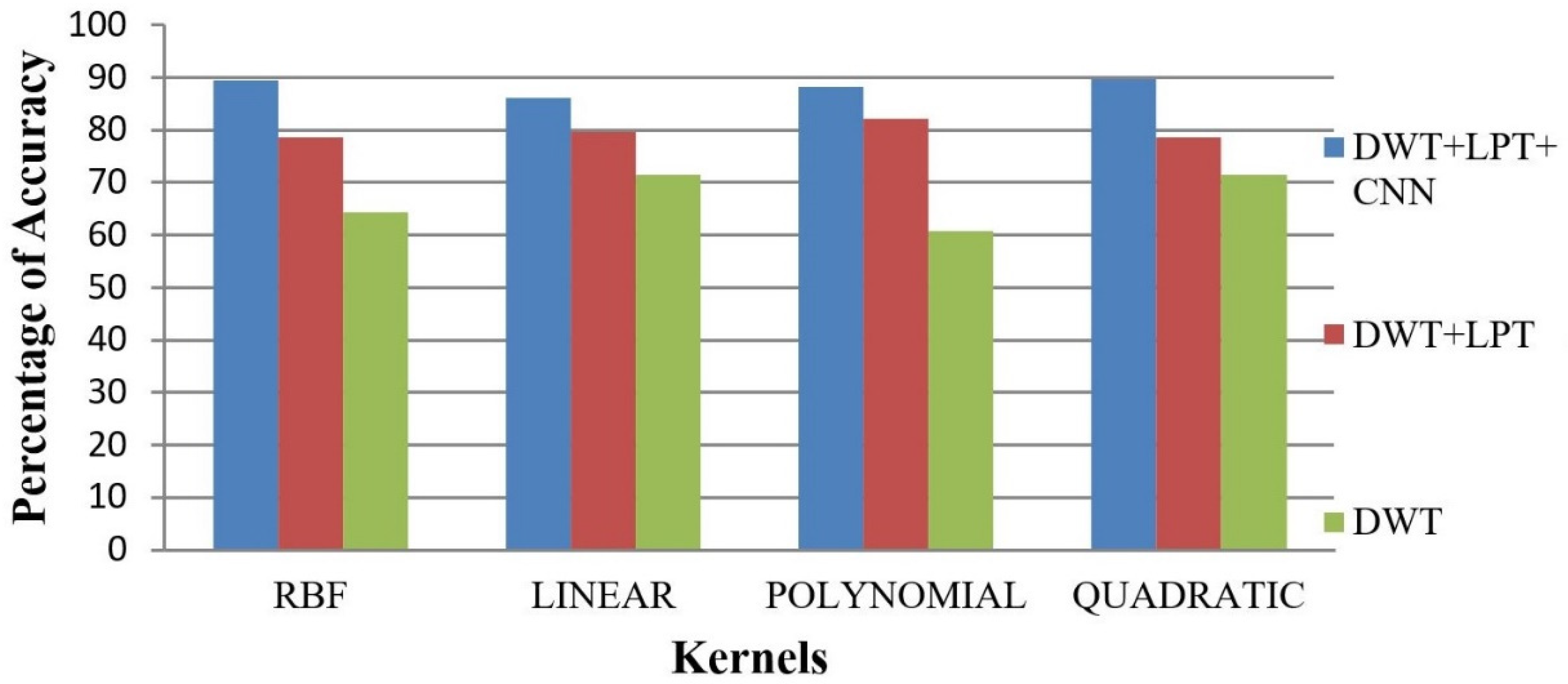
| RBF (%) | Linear (%) | Polynomial (%) | Quadratic (%) | ||
| Abnormality Classification | DWT | 83.29 | 85.97 | 86.37 | 87.49 |
| DWT + LPT | 89.41 | 91.11 | 90.21 | 91.78 | |
| DWT + LPT + CNN | 92.41 | 99.11 | 98.21 | 99.78 | |
| Tumor Classification | DWT | 64.29 | 71.43 | 60.71 | 71.43 |
| DWT + LPT | 78.57 | 79.64 | 82.14 | 78.57 | |
| DWT + LPT + CNN | 89.41 | 86.11 | 88.21 | 89.78 | |
| Classification | Method | T-1 Weighted Images | |||
|---|---|---|---|---|---|
| RBF (%) | Linear (%) | Polynomial (%) | Quadratic (%) | ||
| Abnormality Classification | DWT | 89.29 | 93.75 | 95.09 | 94.94 |
| DWT + LPT | 92.71 | 96.40 | 97.66 | 96.21 | |
| DWT + LPT + CNN | 94.84 | 98.62 | 98.28 | 98.45 | |
| Tumor Classification | DWT | 75.00 | 83.33 | 89.58 | 83.33 |
| DWT + LPT | 85.42 | 89.58 | 93.75 | 93.75 | |
| DWT + LPT + CNN | 91.48 | 94.83 | 97.66 | 97.66 | |
| Classification | Method | T-2 Weighted Images | |||
|---|---|---|---|---|---|
| RBF (%) | Linear (%) | Polynomial (%) | Quadratic (%) | ||
| Abnormality Classification | DWT | 89.51 | 94.20 | 94.53 | 94.59 |
| DWT + LPT | 92.02 | 96.94 | 95.88 | 97.72 | |
| DWT + LPT + CNN | 94.21 | 97.23 | 97.26 | 98.87 | |
| Tumor Classification | DWT | 77.90 | 73.16 | 77.90 | 81.05 |
| DWT + LPT | 80.53 | 81.05 | 82.63 | 84.74 | |
| DWT + LPT + CNN | 91.33 | 93.85 | 95.67 | 97.28 | |
Publisher’s Note: MDPI stays neutral with regard to jurisdictional claims in published maps and institutional affiliations. |
© 2022 by the authors. Licensee MDPI, Basel, Switzerland. This article is an open access article distributed under the terms and conditions of the Creative Commons Attribution (CC BY) license (https://creativecommons.org/licenses/by/4.0/).
Share and Cite
Jibon, F.A.; Khandaker, M.U.; Miraz, M.H.; Thakur, H.; Rabby, F.; Tamam, N.; Sulieman, A.; Itas, Y.S.; Osman, H. Cancerous and Non-Cancerous Brain MRI Classification Method Based on Convolutional Neural Network and Log-Polar Transformation. Healthcare 2022, 10, 1801. https://doi.org/10.3390/healthcare10091801
Jibon FA, Khandaker MU, Miraz MH, Thakur H, Rabby F, Tamam N, Sulieman A, Itas YS, Osman H. Cancerous and Non-Cancerous Brain MRI Classification Method Based on Convolutional Neural Network and Log-Polar Transformation. Healthcare. 2022; 10(9):1801. https://doi.org/10.3390/healthcare10091801
Chicago/Turabian StyleJibon, Ferdaus Anam, Mayeen Uddin Khandaker, Mahadi Hasan Miraz, Himon Thakur, Fazle Rabby, Nissren Tamam, Abdelmoneim Sulieman, Yahaya Saadu Itas, and Hamid Osman. 2022. "Cancerous and Non-Cancerous Brain MRI Classification Method Based on Convolutional Neural Network and Log-Polar Transformation" Healthcare 10, no. 9: 1801. https://doi.org/10.3390/healthcare10091801