Counting Hamiltonian Cycles in 2-Tiled Graphs

Abstract
:1. Introduction
2. Related Research
3. Hamiltonian Cycles in 2-Tiled Graphs
- 1.
- The tiles and are compatible whenever
- 2.
- A sequence of tiles is compatible if, for each , is compatible with .
- 3.
- The join of compatible tiles and is the tile for which the graph is obtained from disjoint union of G and by identifying the sequence y term by term with the sequence .
- 4.
- The join of a compatible sequence of tiles is defined as .
- 5.
- A tile T is cyclically compatible if T is compatible with itself.
- 6.
- For a cyclically compatible tile , the cyclization of T is the graph obtained by identifying the respective vertices of x with y.
- 7.
- A cyclization of a cyclically compatible sequence of tiles is defined as .
- 8.
- A k-tiled graph is a cyclization of a sequence of at least k-tiles.
- 1.
- .
- 2.
- is a union of paths and isolated vertices.
- 3.
- Let v be a vertex of a component of . Then, v has degree 2 in or v is a wall vertex.
- 4.
- There are at most two distinct non-degenerate paths in .
- 5.
- If consists of distinct non-degenerate paths and , then .
- Let K be a component of . As C is a cycle, K is a connected subgraph of C. Then, K is either equal to C, a path, or a vertex. If , then contains all the vertices of G, a contradiction to (in at least one tile, C does not contain all the vertices). The claim follows.
- Let v be a vertex of of degree different from 2. As maximum degree in C is 2, v has degree 1 or 0. If v is an internal vertex of , its degree in is equal to its degree in . This contradicts C being a cycle and the claim follows.
- By Claim 3, paths start and end in a wall vertex. Each distinct non-degenerate path needs two unique wall vertices, and the claim follows.
- By Claim 4, and contain all the wall vertices. By Claim 3, isolated vertices can only be wall vertices; hence, there are no isolated vertices and .
- 1.
- A path that begins in a vertex of the left wall, ends in a vertex of the right wall, and covers all internal vertices of .
- 2.
- A pair of distinct paths for which each begins and ends at opposite walls, span , and respect the vertex order of the walls.
- 3.
- A pair of distinct paths for which each begins and ends at opposite walls, span , and invert the vertex order of the walls.
- 4.
- An empty set.
- 5.
- A pair of distinct paths for which each begins and ends at the same wall and span .
- 6.
- A path that begins and ends at the same wall and covers all internal vertices of .
- 1.
- If a cycle C traverses with a single path and covers all internal vertices of , then we say that is of zigzagging C-type, of which there exist four kinds, relevant for completing the Hamiltonian cycles between the tiles.First, is of zigzagging C-type if contains a single path P, the endvertices of P are vertices and of distinct walls of , and P contains the non-endvertex wall vertices . If either wall vertex that is not an endvertex of P is not contained in P, then contains a path P and these vertices as isolated vertex components. We denote such isolated components using an overline, leading to zigzagging C-types .
- 2.
- If a cycle C traverses with a pair of distinct traversing paths that span , then we say that is of traversing C-type.
- (a)
- is of aligned (Aligned pairs of traversing paths were introduced in [8].) traversing C-type = if contains a pair of distinct paths and , the endvertices of are and , and the endvertices of are and .
- (b)
- is of twisted (Twisted pairs of traversing paths were introduced in [8].) traversing C-type × if contains a pair of distinct paths and , the endvertices of are and , and the endvertices of are and .
- 3.
- If a cycle C does not traverse , then we say that is of flanking C-type.
- (a)
- is of flanking C-type ∅ if is an empty graph spanned by .
- (b)
- is of flanking C-type ‖ if contains a pair of distinct paths and , the endvertices of are and , and the endvertices of are and .
- (c)
- is of flanking C-type if contains a single path P, the endvertices of P are of the same wall of , and P contains the non-endvertex wall vertices . If either wall vertex that is not endvertex of P is not contained in P, then contains a path P and these vertices as isolated components. We denote this using an overline, leading to flanking C-types , , . The respective notations for flanking C-types of P with endvertices are , , ,.
- 1.
- is of zigzagging C-type.
- 2.
- : is of flanking C-type ‖ and , is of traversing C-type.
- 3.
- : and are of compatible flanking C-type of form and , respectively, and , is of traversing C-type.
- 4.
- : are of flanking C-types , ∅, , respectively, and , is of traversing C-type.
- 5.
- is of traversing C-type, where the number of indices i of tiles of traversing C-type × is odd.
- We prove that, if is of zigzagging C-type, then the same holds for and . Suppose that is of zigzagging C-type. Then, has the property that exactly one of its left and one of its right wall vertices have a degree 1 in (the ones that are endvertices of the path from the left to right walls). Because the degree of every vertex in C is 2, the left wall vertex has degree 1 in and the right wall vertex has degree 1 in . Because the degree of every vertex in C is 2, other wall vertices are either of degree 0 (isolated vertex) or 2 (vertex is part of a path) in . If a wall vertex is of degree 0 (2) in , then its degree in (left wall vertex of ) or in (right wall vertex of ) is 2 (0). Hence, based on Corollary 2, and are of zigzagging C-type. By extending the argument to their neighbors, we establish Claim 1 of Lemma 2. For the rest of the proof, we may therefore assume that none of the tiles are of zigzagging C-type.
- Let be of C-type ‖. Let be paths in . Assume without loss of generality that starts in and ends in and that starts in and ends in . Because , , where are paths in , which start in and end in , respectively. Then, , . For , is nontrivial and connected; otherwise, would not be connected. Hence, are vertex disjoint paths in that cover all internal vertices (C is a Hamiltonian cycle) with endvertices in the opposite walls. Therefore, is of traversing C-type. We established Claim 2 of Lemma 2, and for the rest of the proof, we may assume that none of the tiles is of C-type ‖.
- Let be of C-type . Then, consists of some isolated vertices (candidates are ) and path . Because any isolated vertex of is part of a path of a neighbouring tile (in this case, ) and is not the endvertex of this path, there is a path in for which the endvertices are and covers possible isolated nodes of a tile . Hence, is of compatible C-type .We now suppose that is of C-type and that is not of C-type ∅. Then, consists of isolated nodes , and path , where is a path for which the endvertices are . Hence, is of C-type .Because , in both cases, , where are paths in , which start in and end in . Then, , and (similarly as in Item 2 of the proof of Lemma 2) is of traversing C-type. We established Claim 3 of Lemma 2, and for the rest of the proof, we may assume that each tile of C-type has an adjacent tile of C-type ∅.
- Let be of C-type and be of C-type ∅. Then, there exists a path in that covers . Because are isolated vertices in , there is a path in for which the endvertices are and covers these isolated nodes . Hence, is of C-type . Because , , where are paths in , which start in and end in . Then, , and (similarly as in Item 2 of the proof of Lemma 2) is of traversing C-type. We established Claim 4 of Lemma 2, and for the rest of the proof, we may assume that there are no tiles of C-type of form .
- Assume now that there is a tile of C-type of form . Then, as we assumed that there are no tiles of C-type of form , a symmetric argument to Item 3 of the proof of Lemma 2 implies is of C-type ∅ (hence, can only be of C-type ). However, then a symmetric argument to Item 4 of the proof of Lemma 2 implies that is of C-type , a contradiction to the assumption that implies all tiles are either of C-type ∅ or traversing C-type.If there is at least one tile of C-type ∅, then consists of at least two disconnected paths and . However, as C only intersects in wall vertices, C is equal to , a contradiction implying that all the tiles are of traversing C-types.The remaining case is that is of traversing C-type. Therefore, , where each path starts in a left wall vertex and ends in a right wall vertex. Without loss of generality, we may assume that, , are such that , ends in same vertex as starts (if not, we can reindex them). Without loss of generality, we may assume that starts in and in .Each tile of C-type × implies that the path moves from the top left wall vertex to the bottom right wall vertex and from the bottom left wall vertex to the top right wall vertex. In case of an even number of tiles of C-type ×, and are distinct cycles. When this number is odd, is a Hamiltonian cycle.
3.1. Counting Traversing Hamiltonian Cycles
3.2. Counting Flanking Hamiltonian Cycles
- ,
- be number of distinct possibilities for to be of compatible flanking C-types to turn around a cycle in .
- We calculate the value .
- Using the idea from the proof for traversing Hamiltonian cycles over the sequence , we getwhere is as in (1). Then, presents the number of different combinations of with an even number of tiles of traversing C-type × and presents the number of different combinations of with an odd number of tiles of traversing C-type ×.
- The number of Hamiltonian cycles turning around in is equal to
- cycle turns around in one tile,
- cycle turns around in two consecutive tiles, and
- cycle turns around in three consecutive tiles.
- Counting flanking Hamiltonian cycles that turn around in one tile:Flanking Hamiltonian cycles that turn around in one tile consist of two parts. One tile is of C-type ‖; other tiles are of traversing C-type. Using Lemma 4 with and , we get the desired result.
- Counting flanking Hamiltonian cycles that turn around in two consecutive tiles:In consecutive tiles and , we have and . Let denote the number of distinct possibilities for and to be of compatible flanking C-types of the forms and . Then,Flanking Hamiltonian cycles that turn around in two consecutive tiles consist of two parts. In consecutive tiles, compatible C-types of forms and are used and other tiles are of traversing C-type. Using Lemma 4 with and , we get the desired result.
- Counting flanking Hamiltonian cycles that turn around in three consecutive tiles:Considering three consecutive tiles , , and implies , , and . Let denote the number of distinct possibilities to turn around in three consecutive tiles , , and . Then,whereFlanking Hamiltonian cycles that turn around in three consecutive tiles consist of two parts. In consecutive tiles , and , respectively, the C-types that are used are , ∅, and . Other tiles are of traversing C-type. Using Lemma 4 with and , we get the desired result.
3.3. Counting Zigzagging Hamiltonian Cycles
- is an endvertex of a path and is part of a path (notation ),
- is an endvertex of a path and is part of a path (notation ),
- is an endvertex of a path and is an isolated vertex (notation ),
- is an endvertex of a path and is an isolated vertex (notation ).
- for :
- for :
- for :
- for :
4. Large 2-Crossing-Critical Graphs as 2-Tiled Graphs
4.1. Characterization of 2-Crossing-Critical Graphs
- 1.
- Crossing number of a graph G is the lowest number of edge crossings of a plane drawing of the graph G.
- 2.
- For a positive integer c, a graph G is c-crossing-critical if the crossing number is at least c but every proper subgraph H of G has .
- 1.
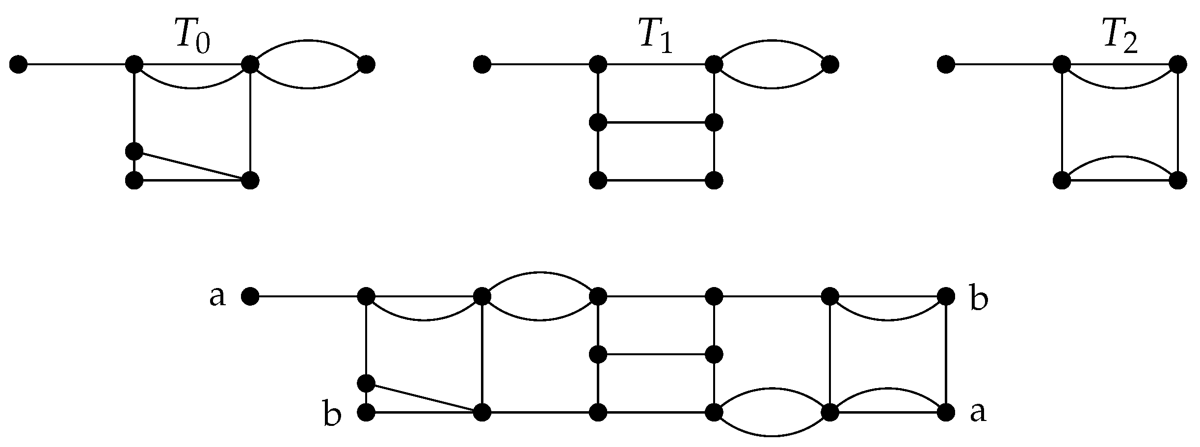
- is 3-connected, contains a subdivision of, and has a very particular twisted Möbius band tile structure, with each tile isomorphic to one of 42 possibilities. All such structures are 3-connected and 2-crossing-critical.
- 2.
- G is 3-connected, does not have a subdivision of , and has at most 3 million vertices.
- 3.
- G is not 3-connected and is one of 49 particular examples.
- 4.
- G is 2-but not 3-connected and is obtained from a 3-connected, 2-crossing-critical graph by replacing digons by digonal paths.
4.2. Construction of Large 2-Crossing-Critical Graphs
- 1.
- For a sequence x, denotes the reversed sequence.
- 2.
- (a) The right-inverted tile of a tile is the tile .(b) The left-inverted tile of a tile is the tile .(c) The inverted tile of a tile is the tile .
- 3.
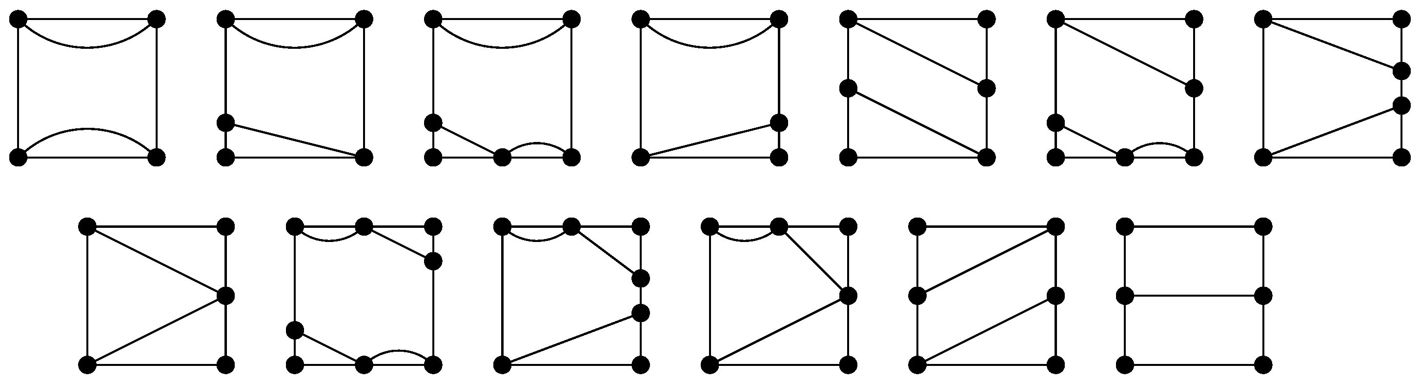
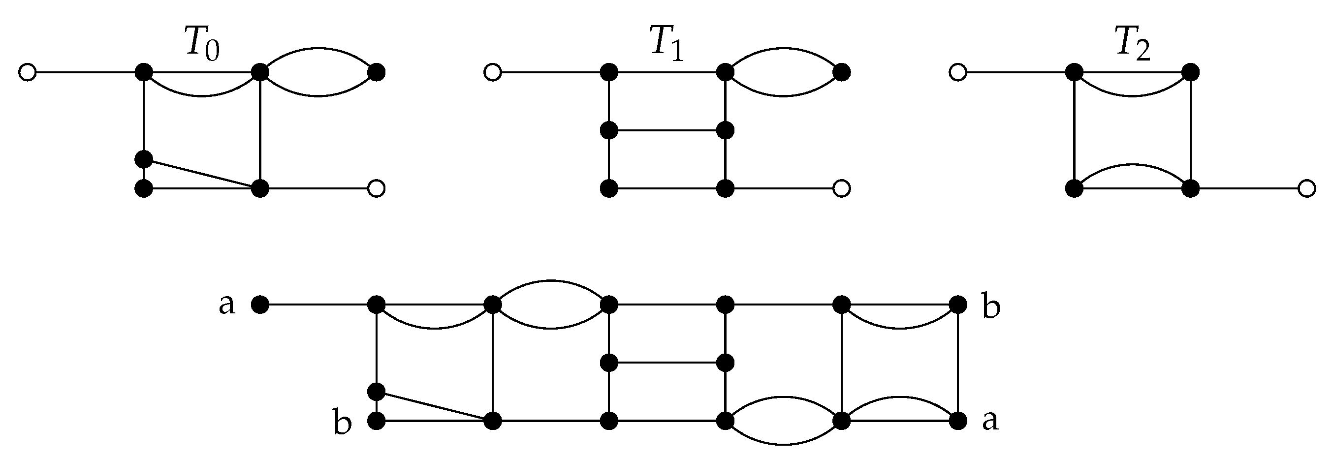
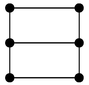
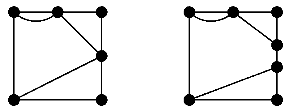
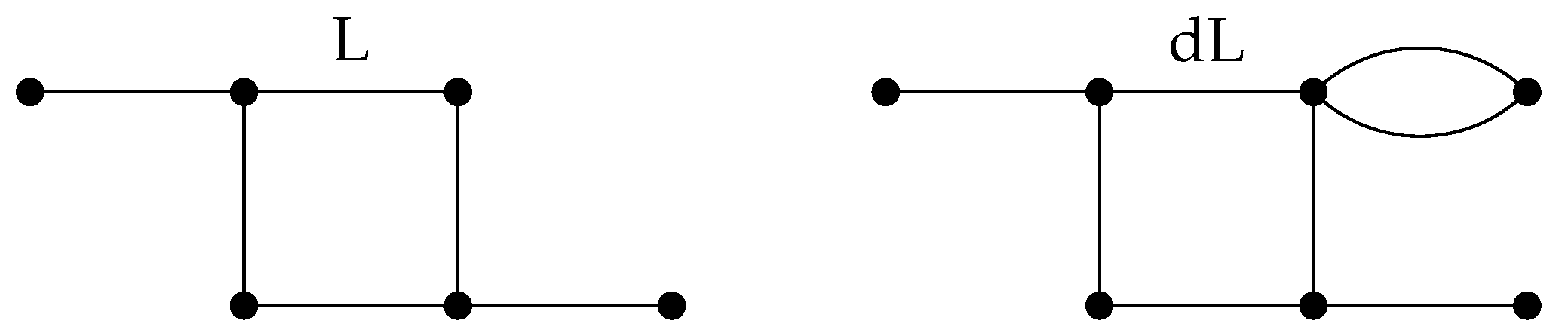
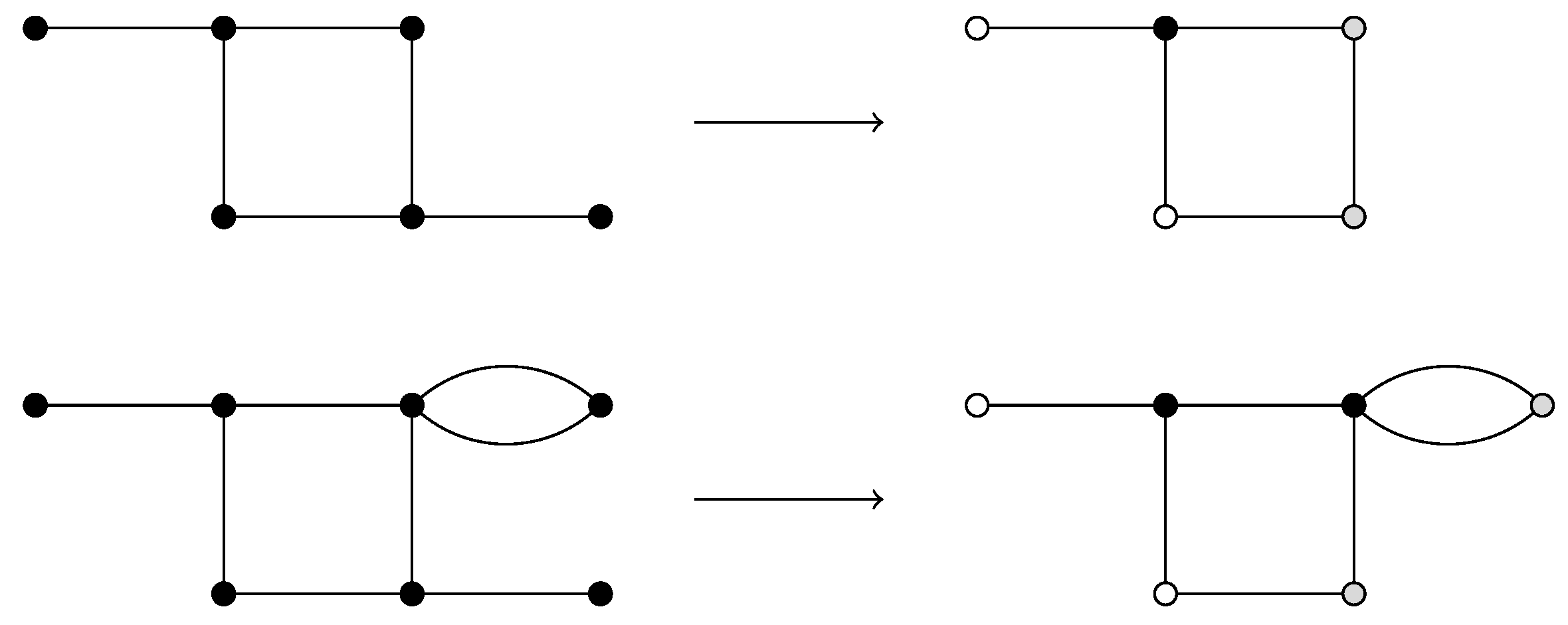
- The set of tiles consists of those tiles obtained as combinations of two frames, shown in Figure 2, and 13 pictures, shown in Figure 3, in such a way that a picture is inserted into a frame by identifying the two geometric squares. (This typically involves subdividing the frame’s square.) A given picture may be inserted into a frame either with the given orientation or with a rotation.
- 4.
- The set consists of all graphs of the form , where is a sequence such that and .
4.3. The Alphabet Describing Tiles
- for , #X is the number of occurrences of X in ;
- for and , is the number of occurrences of X in ; and
- for , and , is the number of occurrences of X as .
5. Hamiltonian Cycles in Large 2-Crossing-Critical Graphs
- is the number of traversing Hamiltonian cycles in G,
- is the number of possibilities for to be of C-type =,
- is the number of possibilities for to be of C-type ‖,
- is the number of distinct possibilities for and to be of compatible flanking C-types of forms and .
- 1.
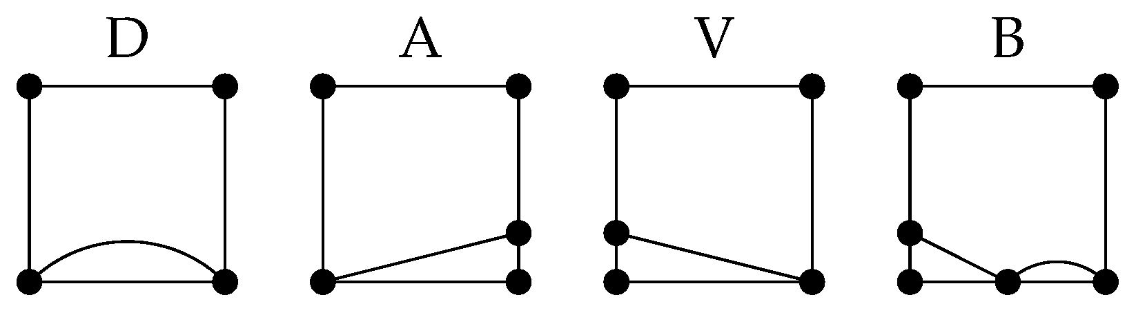
- Let . Using Figure 13, it is easy to see thatFor , all pictures except H are valid, and paths B and D add a multiplier 2. Hence,For , all pictures except H are valid, and paths B and D, and the frame add a multiplier 2. Hence,
- 2.
- Let . Using Figure 14, it is easy to see thatFor , all pictures except H are valid, and paths B and D add a multiplier 2. Hence,For , there are several options:
- The bottom path is V; the top path is any of the possible ones; and top paths B and D, and the frame add a multiplier 2.
- The bottom path is B; the top path is any of the possible ones; and the bottom path B, top paths B and D, and the frame add a multiplier 2.
- The top path is V; the bottom path is any of the possible ones, except B; and the frame adds a multiplier 2.
- The top path is H, and the frame adds a multiplier 2.
The first and the third options both cover the picture with the top path V and the bottom path V. Hence,For , there are several options:- The top path is V; the bottom path is any of the possible ones; and the bottom paths B and D add a multiplier 2.
- The top path is B; the bottom path is any of the possible ones; and the top path B and bottom paths B and D add a multiplier 2.
- The bottom path is V, and the top path is any of the possible ones, except B.
- The top path is H.
The first and the third options both cover the picture with top path V and bottom path V. Hence,For , all pictures except H are valid, and paths B and D, and the frame add a multiplier 2. Hence,
- Tile with frame L:where (frame adds a factor 1 and pictures add a factor 2).
- Tile with frame :where (frame adds a factor 2 and pictures add a factor 2).
- Tile with frame L:where and so .
- Tile with frame :where and so .
Author Contributions
Funding
Institutional Review Board Statement
Informed Consent Statement
Data Availability Statement
Conflicts of Interest
Appendix A

| Notation | Description |
|---|---|
| Set of all possible zigzagging C-types. | |
| Set of all possible traversing C-types. | |
| Set of all possible flanking C-types. | |
| Set of all possible C-types. | |
| Number of possibilities for tile to be of C-type . | |
| Number of distinct possibilities in with even number of tiles of C-type × | |
| and all others of C-type =. | |
| Number of distinct possibilities in with odd number of tiles of C-type × | |
| and all other of C-type =. | |
| Notation for matrix | |
| Represents the join . | |
| Number of distinct possibilities for to be of compatible flanking C-types to turn | |
| around a cycle in , . | |
| Number of distinct possibilities for and to be of compatible flanking C-types of form | |
| and . | |
| Number of distinct possibilities to turn around in three consecutive tiles and . | |
| Notation for matrix | |
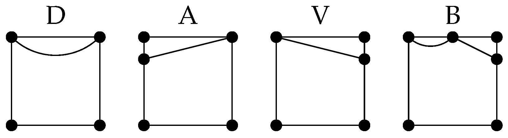
| Describes the top path of the tile. | |
| Describes if the top and bottom paths of the tile intersect. | |
| Describes the bottom path of the tile. | |
| Describes the frame used for the tile. | |
| The number of occurences of X in . | |
| The number of occurences of X in . | |
| The number of occurences of X in . | |
| The number of traversing Hamiltonian cycles in . | |
| The number of flanking Hamiltonian cycles in . | |
| The number of zigzagging Hamiltonian cycles in . |
References
- Kuratowski, C. Sur le probleme des courbes gauches en Topologie. Fundam. Math. 1930, 15, 271–283. [Google Scholar] [CrossRef]
- Bollobas, B. Combinatorics: Set Systems, Hypergraphs, Families of Vectors and Probabilistic Combinatorics; Cambridge University Press: New York, NY, USA, 1986. [Google Scholar]
- Trotter, W.T., Jr.; Moore, J.I., Jr. Characterization problems for graphs, partially ordered sets, lattices, and families of sets. Discret. Math. 1976, 16, 361–381. [Google Scholar] [CrossRef] [Green Version]
- Chudnovsky, M.; Robertson, N.; Seymour, P.; Thomas, R. The strong perfect graph theorem. Ann. Math. 2006, 164, 51–229. [Google Scholar] [CrossRef] [Green Version]
- Lovász, L. A characterization of perfect graphs. J. Comb. Theory Ser. B 1972, 13, 95–98. [Google Scholar] [CrossRef] [Green Version]
- Archdeacon, D. A Kuratowski theorem for the projective plane. J. Graph Theory 1981, 5, 243–246. [Google Scholar] [CrossRef] [Green Version]
- Robertson, N.; Seymour, P.D. Graph minors. VIII. A Kuratowski theorem for general surfaces. J. Comb. Theory, Ser. B 1990, 48, 255–288. [Google Scholar] [CrossRef] [Green Version]
- Bokal, D.; Oporowski, B.; Richter, R.B.; Salazar, G. Characterizing 2-crossing-critical graphs. Adv. Appl. Math. 2016, 74, 23–208. [Google Scholar] [CrossRef]
- des Cloizeaux, J.; Jannik, G. Polymers in Solution: Their Modelling and Structure; Clarendon Press: Oxford, MS, USA, 1990. [Google Scholar]
- Bašić, N.; Bokal, D.; Boothby, T.; Rus, J. An algebraic approach to enumerating non-equivalent double traces in graphs. MATCH Commun. Math. Comput. Chem. 2017, 78, 581–594. [Google Scholar]
- Gradišar, H.; Božič, S.; Doles, T.; Vengust, D.; Hafner-Bratkovič, I.; Mertelj, A.; Webb, B.; Šali, A.; Klavžar, S.; Jerala, R. Design of a single-chain polypeptide tetrahedron assembled from coiled-coil segments. Nat. Chem. Biol. 2013, 9, 362–366. [Google Scholar] [CrossRef] [PubMed] [Green Version]
- Tošić, R.; Bodroža-Pantić, O.; Kwong, Y.H.H.; Straight, H.J. On the number of Hamiltonian cycles of P4 × Pn. Indian J. Pure Appl. Math. 1990, 21, 403–409. [Google Scholar]
- Kwong, Y.H.H.; Rogers, D.G. A matrix method for counting Hamiltonian cycles on grid graphs. Eur. J. Comb. 1994, 15, 277–283. [Google Scholar] [CrossRef] [Green Version]
- Bodroža-Pantić, O.; Tošič, R. On the number of 2-factors in rectangular lattice graphs. Publ. De L’Institut Math. 1994, 56, 23–33. [Google Scholar]
- Stoyan, R.; Strehl, V. Enumeration of Hamiltonian circuits in rectangular grids. J. Comb. Math. Comb. Comput. 1996, 21, 109–127. [Google Scholar]
- Bodroža-Pantić, O.; Kwong, H.; Doroslovački, R.; Pantić, M. Enumeration of Hamiltonian cycles on a thick grid cylinder—Part I: Non-contractible Hamiltonian cycles. Appl. Anal. Discret. Math. 2019, 13, 28–60. [Google Scholar] [CrossRef] [Green Version]
- Bodroža-Pantić, O.; Pantić, B.; Pantić, I.; Bodroža-Solarov, M. Enumeration of Hamiltonian cycles in some grid graphs. MATCH Commun. Math. Comput. Chem. 2013, 70, 181–204. [Google Scholar]
- Higuchi, S. Field theoretic approach to the counting problem of Hamiltonian cycles of graphs. Phys. Rev. E 1998, 58, 128–132. [Google Scholar] [CrossRef] [Green Version]
- Higuchi, S. Counting Hamiltonian cycles on planar random lattices. Mod. Phys. Lett. A 1998, 13, 727–733. [Google Scholar] [CrossRef] [Green Version]
- Frieze, A.; Jerrum, M.; Molloy, M.; Robinson, R.; Worml, N. Generating and counting Hamilton cycles in random regular graphs. J. Algorithms 1996, 21, 176–198. [Google Scholar] [CrossRef]
- Fallon, J.E. Two Results in Drawing Graphs on Surfaces. Doctoral Dissertation, Louisiana State University and Agricultural and Mechanical College, Baton Rouge, LA, USA, 2018. retrived from LSU Digital Commons. [Google Scholar]
- Goodman, S.; Hedetniemi, S. Sufficient conditions for a graph to be Hamiltonian. J. Comb. Theory Ser. B 1974, 16, 175–180. [Google Scholar] [CrossRef] [Green Version]
- Faudree, R.J.; Gould, R.J. Characterizing forbidden pairs for Hamiltonian properties. Discret. Math. 1997, 173, 45–60. [Google Scholar] [CrossRef] [Green Version]
- Faudree, R.J.; Gould, R.; Jacobson, M. Forbidden triples implying Hamiltonicity: For all graphs. Discuss. Math. Graph Theory 2004, 24, 47–54. [Google Scholar] [CrossRef]
- Gagarin, A.; Myrvold, W.; Chambers, J. Forbidden minors and subdivisions for toroidal graphs with no K3,3’s. Electron. Notes Discret. Math. 2005, 22, 151–156. [Google Scholar] [CrossRef]
- Mohar, B. A linear time algorithm for embedding graphs in an arbitrary surface. SIAM J. Discret. Math. 1999, 12, 6–26. [Google Scholar] [CrossRef] [Green Version]
- Kawarabayashi, K.; Mohar, B.; Reed, B. A simpler linear time algorithm for embedding graphs into an arbitrary surface and the genus of graphs of bounded tree-width. In Proceedings of the 49th Annual IEEE Symposium on Foundations of Computer Science, Philadelphia, PA, USA, 23–25 October 2008; pp. 771–780. [Google Scholar]
- Chartr, G.; Geller, D.; Hedetniemi, S. Graphs with forbidden subgraphs. J. Comb. Theory Ser. B 1971, 10, 12–41. [Google Scholar] [CrossRef] [Green Version]
- Dvořák, Z. On forbidden subdivision characterizations of graph classes. Eur. J. Comb. 2008, 29, 1321–1332. [Google Scholar] [CrossRef] [Green Version]
- Šiřan, J. Infinite families of crossing-critical graphs with a given crossing number. Discret. Math. 1984, 48, 129–132. [Google Scholar] [CrossRef] [Green Version]
- Kochol, M. Construction of crossing-critical graphs. Discret. Math. 1987, 66, 311–313. [Google Scholar] [CrossRef] [Green Version]
- Pinontoan, B.; Richter, R.B. Crossing numbers of sequence of graphs I: General tiles. Aust. J. Comb. 2004, 30, 197–206. [Google Scholar]
- Szalazar, G. Infinite families of crossing-critical graphs with given average degree. Discret. Math. 2003, 271, 343–350. [Google Scholar] [CrossRef] [Green Version]
- Hlineny, P. New infinite families of almost-planar crossing-critical graphs. Electron. J. Comb. 2008, 15, R102:1–12. [Google Scholar]
- Bokal, D.; Bračič, M.; Derňár, M.; Hliněný, P. On degree properties of crossing-critical families of graphs. Electron. J. Comb. 2019, 26, P153:1–28. [Google Scholar] [CrossRef]
- Dvořák, Z.; Hliněný, P.; Mohar, B. Structure and generation of crossing-critical graphs. In Proceedings of the 34th International Symposium on Computational Geometry, Budapest, Hungary, 11–14 June 2018; pp. 33:1–33:14. [Google Scholar]
- Bokal, D.; Dvořák, Z.; Hliněný, P.; Leanos, J.; Mohar, B.; Wiedera, T. Bounded degree conjecture holds precisely for c-crossing-critical graphs with c≤12. In Proceedings of the 35th International Symposium on Computational Geometry, Portland, OR, USA, 18–21 June 2019; pp. 14:1–14:15. [Google Scholar]
- Dvořák, Z.; Mohar, M. Crossing-critical graphs with large maximum degree. J. Comb. Theory Ser. B 2010, 100, 413–417. [Google Scholar] [CrossRef] [Green Version]
- Dvořák, Z.; Mohar, M. Crossing numbers of periodic graphs. J. Graph Theory 2015, 83, 34–43. [Google Scholar] [CrossRef] [Green Version]
- Bokal, D.; Chimani, M.; Nover, A.; Schierbaum, J.; Stolzmann, T.; Wagner, M.H.; Wiedera, T. Invariants in large 2-crossing-critical graphs. J. Graph Algorithms Appl. under review.
- Lovász, L. Large Networks and Graph Limits; American Mathematical Society: Providence, RI, USA, 2012. [Google Scholar]
- Bokal, D. Infinite families of crossing-critical graphs with prescribed average degree and crossing number. J. Graph Theory 2010, 65, 139–162. [Google Scholar] [CrossRef]
- Žerak, T.; Bokal, D. Playful introduction to 2-crossing-critical graphs. Dianoia 2019, 3, 101–108. [Google Scholar]


Publisher’s Note: MDPI stays neutral with regard to jurisdictional claims in published maps and institutional affiliations. |
© 2021 by the authors. Licensee MDPI, Basel, Switzerland. This article is an open access article distributed under the terms and conditions of the Creative Commons Attribution (CC BY) license (http://creativecommons.org/licenses/by/4.0/).
Share and Cite
Vegi Kalamar, A.; Žerak, T.; Bokal, D. Counting Hamiltonian Cycles in 2-Tiled Graphs. Mathematics 2021, 9, 693. https://doi.org/10.3390/math9060693
Vegi Kalamar A, Žerak T, Bokal D. Counting Hamiltonian Cycles in 2-Tiled Graphs. Mathematics. 2021; 9(6):693. https://doi.org/10.3390/math9060693
Chicago/Turabian StyleVegi Kalamar, Alen, Tadej Žerak, and Drago Bokal. 2021. "Counting Hamiltonian Cycles in 2-Tiled Graphs" Mathematics 9, no. 6: 693. https://doi.org/10.3390/math9060693