Geometrically Constructed Family of the Simple Fixed Point Iteration Method

Abstract

This study presents a new one-parameter family of the well-known fixed point iteration method for solving nonlinear equations numerically. The proposed family is derived by implementing approximation through a straight line. The presence of an arbitrary parameter in the proposed family improves convergence characteristic of the simple fixed point iteration as it has a wider domain of convergence. Furthermore, we propose many two-step predictor–corrector iterative schemes for finding fixed points, which inherit the advantages of the proposed fixed point iterative schemes. Finally, several examples are given to further illustrate their efficiency.

1. Introduction

The fixed point iteration is probably the simplest and most important root-finding algorithm in numerical analysis [1,2]. The fixed point methods and fixed point theorems have many applications in mathematics and engineering. One way to study numerical ordinary differential solvers and Runge–Kutta methods is to convert them as fixed point iterations. The well-known Newton’s method [2,3,4,5,6,7,8,9,10,11,12,13,14,15,16,17] is also a special case of an iteration method. The fixed point theory has been voluminously used as a tool to find the solution of function-differential equations. Furthermore, the fixed point problems are equivalent to root-finding problems and sometimes easier to analyze while posing some strange and cute problems by themselves.

Suppose that we wish to find the approximate solution of the nonlinear equation

$$f\left(x\right)=0,$$

(1)

where $f:[a,b]\subset \mathbb{R}\to \mathbb{R}$ is a sufficiently differentiable function with simple zeros.

This can be rewritten to obtain an equation of the form

$$x=\varphi \left(x\right),$$

(2)

in such a way that any solution of (2), which is a fixed point, is a root of the original Equation (1). Root-finding problems and fixed-point problems are equivalent classes in the following sense:

$$f\left(x\right)\mathrm{has}\mathrm{a}\mathrm{zero}\mathrm{at}x=\alpha \iff \varphi \left(x\right)=x-f\left(x\right)\mathrm{has}\mathrm{a}\mathrm{fixed}\mathrm{point}\mathrm{at}x=\alpha .$$

Geometrically, the fixed point occurs where the graph of $y=\varphi \left(x\right)$ intersects the graph of the straight line $y=x$. Starting from a suitable approximation $x_0$ and consider that the recursive process:

$$x_{n+1}=\varphi \left(x_n\right),n\ge 0,1,2,\cdots ,$$

(3)

is called a fixed point iteration method. This method is locally linearly convergent if $|{\varphi }^{\prime }\left(x\right)|<1$ for all $x\in [a,b]$.

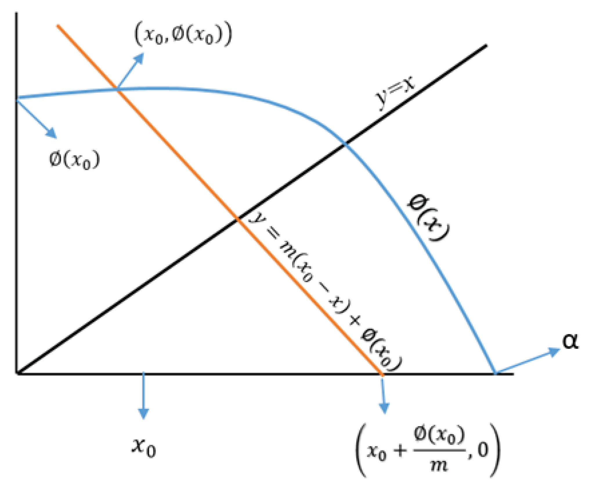
2. Geometric Derivation of the Family

Assume that Equation (2) has a fixed point at $x=\alpha$. Let

$$y=\varphi \left(x\right)$$

(4)

represent the graph of the function $\varphi \left(x\right)$.

Let $x_0$ be an initial guess to the required fixed point and $\varphi \left(x_0\right)$ be the corresponding point on the graph of the function $y=\varphi \left(x\right)$. The idea is to approximate nonlinear function $y=\varphi \left(x\right)$ by a linear approximation. Therefore, we assume that

$$(y-\varphi (x_0\left)\right)+m(x-x_0)=0$$

(5)

be a linear approximation to the curve $y=\varphi \left(x\right)$, where $m\ge 0$ is the slope of the straight line. The expression (5) can be rewritten as $y=m(x_0-x)+\varphi \left(x_0\right)$, and this line is passing through the points $(x_0,\varphi \left(x_0\right))$ and $\left(x_0+\frac{\varphi \left(x_0\right)}{m},0\right)$. More details can be found in the following Figure 1:

The point of intersection of (5) with the straight line $y=x$ will be a required fixed point and let $x=x_1$ be this point of intersection. Therefore, at the point of intersection, the expression (5) yields

$$x_1=\frac{m{x}_0+\varphi \left(x_0\right)}{m+1}.$$

(6)

Without loss of generality, the general form of the above expression (6) can be written as follows:

$$x_{n+1}=\frac{m{x}_n+\varphi \left(x_n\right)}{m+1},n\ge 0.$$

(7)

Next, we want to demonstrate the convergence order of the proposed iterative scheme (7). Therefore, we rewrite the expression (7) in the following way:

$$x_{n+1}=\frac{m{x}_n+\varphi \left(x_n\right)}{m+1}=h\left(x_n\right),$$

or we can say that $h\left(x\right)={\displaystyle \frac{mx+\varphi \left(x\right)}{m+1}}$. If $\alpha$ is a fixed point of $\varphi \left(x\right)=x$, then

$$h\left(\alpha \right)=\frac{m\alpha +\varphi \left(\alpha \right)}{m+1}=\frac{m\alpha +\alpha }{m+1}=\alpha .$$

So, we conclude that $\alpha$ is a root of $h\left(x\right)=0$.

Theorem 1.

Let $\varphi \left(x\right)$ and ${\varphi }^{\prime }\left(x\right)$ be continuous functions on the interval $[a,b]$. In addition, we assume that $m\ge 0$ and $a\le x\le b\Rightarrow a\le \varphi \left(x\right)\le b,\lambda =max\left\{\right|h^{\prime }\left(x\right)\left|\right\}$ for all $x\in [a,b]$, then (i) $x=h\left(x\right)$ has a unique solution $\alpha \in [a,b]$; (ii) for any initial guess $x_0\in [a,b]$, the iteration $x_{n+1}=h\left(x_n\right),n=0,1,2,\cdots$ will converge to α.

Proof. 

First of all, we will prove the first part. Since ${\varphi }^{\prime }\left(x\right)$ exists in the interval $[a,b]$, therefore, this implies that $h^{\prime }\left(x\right)$ exists in the interval $[a,b]$. For any two points $u,v\in [a,b]$, we have

$$h\left(u\right)-h\left(v\right)=h^{\prime }\left(c\right)(u-v),\mathrm{for}\mathrm{some}c\in (u,v),$$

which yields further

$$\begin{array}{cc}\hfill \left|h\right(u)-h(v\left)\right|& =|h^{\prime }\left(c\right)\left|\right|u-v|,\hfill \\ \hfill & \le \lambda |u-v|.\hfill \end{array}$$

(8)

Let us suppose that there are two solutions $\alpha$ and $\beta$ of $x=h\left(x\right)$ in the interval $[a,b]$. So, we have

$$h\left(\alpha \right)=\alpha ,\mathrm{and}h\left(\beta \right)=\beta .$$

From (8), we further have

$$\left|h\right(\alpha )-h(\beta \left)\right|\le \lambda |\alpha -\beta |.$$

If $\alpha \ne \beta$, then $\lambda \ge 1$ which contradicts the fact that $\lambda <1$. Therefore, we have

$$\alpha =\beta .$$

Hence, $x=h\left(x\right)$ has a unique solution in [a, b].

Next, we move to the second part.

If $x_0\in [a,b]$, then $\varphi \left(x_0\right)\in [a,b]$. This further implies that

$$\frac{m{x}_0+\varphi \left(x_0\right)}{(m+1)}\in [a,b].$$

Therefore, $h\left(x_0\right)\in [a,b]$ and hence $x_1\in [a,b]$.

Repeating the above process inductively, one gets $\left\{x_n\right\}\in [a,b]$.

Furthermore, one can have

$$\begin{array}{cc}\hfill |x_n-\alpha |& =|h\left(x_{n-1}\right)-h\left(\alpha \right)|,\hfill \\ \hfill & =|h^{\prime }\left(c_n\right)\left|\right|x_{n-1}-\alpha |,\mathrm{for}\mathrm{some}{c}_n\in (\alpha ,x_{n-1}),\hfill \\ \hfill & \le \lambda |x_{n-1}-\alpha |.\hfill \end{array}$$

Continuing inductively

$$|x_n-\alpha |\le {\lambda }^n|x_0-\alpha |\to 0,(\mathrm{as}\lambda <1)$$

Hence, the sequence $\left\{x_n\right\}$ of $x_{n+1}=h\left(x_n\right)$ converges to $\alpha$. □

Theorem 2.

Let $\varphi :\mathbb{R}\to \mathbb{R}$ be an analytic function in the region containing the fixed point $x=\alpha$. In addition, we assume that initial guess $x=x_0$ is sufficiently close to the required fixed point for guaranteed convergence. Then, the proposed scheme (7) has at least linear convergence

$$e_{n+1}={\displaystyle \frac{(m+{\varphi }^{\prime }\left(\alpha \right))e_n}{m+1}}+{\displaystyle \frac{{\varphi }^{″}\left(\alpha \right)e_n^2}{m+1}}+O\left(e_n^3\right).$$

In the case $m=-{\varphi }^{\prime }\left(\alpha \right)\approx -{\varphi }^{\prime }\left(x_n\right)\approx -\left({\displaystyle \frac{\varphi \left(x_{n+1}\right)-\varphi \left(x_n\right)}{x_{n+1}-x_n}}\right)$, we obtain

$$m=-\left(\frac{\varphi \left(\varphi \left(x_n\right)\right)-\varphi \left(x_n\right)}{\varphi \left(x_n\right)-x_n}\right),$$

(9)

since $x_{n+1}=\varphi \left(x_n\right)$, then the scheme (7) reaches at least the second order of convergence.

Proof. 

Suppose $x_n\approx \alpha$. We can write

$$h\left(x_n\right)=h\left(\alpha \right)+h^{\prime }\left(\alpha \right)(x_n-\alpha )+h^{″}\left(\alpha \right)\frac{{(x_n-\alpha )}^2}{2!}+O\left({(x_n-\alpha )}^3\right),$$

by Taylor’s expansion in the neighborhood of fixed point “$\alpha$”.

Therefore, one gets

$$x_{n+1}-\alpha =h^{\prime }\left(\alpha \right)(x_n-\alpha )+h^{″}\left(\alpha \right)\frac{{(x_n-\alpha )}^2}{2!}+O\left({(x_n-\alpha )}^3\right).$$

(10)

As $h\left(x\right)={\displaystyle \frac{mx+\varphi \left(x\right)}{m+1}}$, we get $h^{\prime }\left(\alpha \right)={\displaystyle \frac{m+{\varphi }^{\prime }\left(\alpha \right)}{m+1}}$ and $h^{″}\left(\alpha \right)={\displaystyle \frac{{\varphi }^{″}\left(\alpha \right)}{m+1}}$.

Substituting these values in (10), one can have

$$e_{n+1}={\displaystyle \frac{(m+{\varphi }^{\prime }\left(\alpha \right))e_n}{m+1}}+{\displaystyle \frac{{\varphi }^{″}\left(\alpha \right)e_n^2}{m+1}}+O\left(e_n^3\right).$$

Furthermore, if $m=-{\varphi }^{\prime }\left(\alpha \right)$, then $e_{n+1}={\displaystyle \frac{{\varphi }^{″}\left(\alpha \right)e_n^2}{m+1}}+O\left(e_n^3\right)$.

This implies that scheme (7) has at least second-order convergence. □

Special Cases

Here, we shall consider the role of the parameter $m\ge 0$ and derive the various following formulas as follows:

1.

For $m=0$, Formula (7) corresponds to the classical fixed point method $x_{n+1}=\varphi \left(x_n\right)$.

2.

For $m={\displaystyle \frac{1-\gamma }{\gamma }}$, where $\gamma \in (0,1]$, Formula (7) corresponds to the following well-known Schaefer’s iteration scheme [18]

$$x_{n+1}=(1-\gamma )x_n+\gamma \varphi \left(x_n\right).$$

3.

For $m={\displaystyle \frac{1-{\gamma }_n}{{\gamma }_n}}$, where $\left\{{\gamma }_n\right\}$ is a real sequence in $(0,1]$, Formula (7) corresponds to the following well-known Mann’s iteration [19]

$$x_{n+1}=(1-{\gamma }_n)x_n+{\gamma }_n\varphi \left(x_n\right).$$

4.

By inserting $m=1$, in scheme (7), one achieves the following well-known Kranselski’s iteration [20]

$$x_{n+1}=\frac{x_n+\varphi \left(x_n\right)}{2},$$

denoted by $\left(KM\right)$ for the computational results (see also more recent work on this iteration in the book [21]).

Similarly, we can derive several other formulas by taking different specific values of m. Furthermore, we proposed the following new schemes on the basis of some standard means of two quantities $x_n$ and $\varphi \left(x_n\right)$ of same signs:

5.

Geometric mean-based fixed point formula is given by

$$x_{n+1}=\sqrt{x_n\varphi \left(x_n\right)},\mathrm{where}{x}_0\ne 0.$$

6.

Harmonic mean-based fixed point formula is defined by

$$x_{n+1}=\frac{2x_n\varphi \left(x_n\right)}{x_n+\varphi \left(x_n\right)},\mathrm{where}{x}_0\ne 0.$$

7.

Centroidal mean-based fixed point formula is mentioned as follows:

$$x_{n+1}=\frac{2\left(x_n^2+x_n\varphi \left(x_n\right)+{\varphi }^2\left(x_n\right)\right)}{3\left(x_n+\varphi \left(x_n\right)\right)}.$$

8.

The following fixed point formula based on the Heronian mean is defined as

$$x_{n+1}=\frac{x_n+\sqrt{x_n\varphi \left(x_n\right)}+\varphi \left(x_n\right)}{3}.$$

9.

The fixed point formula based on Contra-harmonic is depicted as follows:

$$x_{n+1}=\frac{x_n^2+{\varphi }^2\left(x_n\right)}{x_n+\varphi \left(x_n\right)}.$$

Remark 1.

Geometric mean-based fixed point formula and Heronian mean formula are applicable for finding positive fixed points only.

3. Two-Step Iterative Schemes

In this section, we present a new two-step predictor–corrector iterative schemes using the modified fixed point methods as predictor. There are several two-point [1,22,23] and multi-point [24,25] iterative schemes in the literature for finding the fixed points. Here, we mention some of them as follows:

1.

Ishikawa [22] has proposed the following iterative scheme:

$$\begin{array}{cc}\hfill x_{n+1}& =(1-{\beta }_n)x_n+{\beta }_n\varphi \left(y_n\right),\hfill \\ \hfill y_n& =(1-{\gamma }_n)x_n+{\gamma }_n\varphi \left(x_n\right),\hfill \end{array}$$

(11)

where $\left\{{\beta }_n\right\}$ and $\left\{{\gamma }_n\right\}$ are sequences of positive numbers in $(0,1]$ as a generalization of the Mann [19] iteration scheme. We denote this method as $\left(IS\right)$ for the computational work and choose ${\beta }_n={\gamma }_n=\frac{1}{n^3+1}$.

2.

Agarwal et al. [1] have proposed the following iteration scheme defined as

$$\begin{array}{cc}\hfill x_{n+1}& =(1-{\beta }_n)\varphi \left(x_n\right)+{\beta }_n\varphi \left(y_n\right),\hfill \\ \hfill y_n& =(1-{\gamma }_n)x_n+{\gamma }_n\varphi \left(x_n\right),\hfill \end{array}$$

(12)

where $\left\{{\beta }_n\right\}$ and $\left\{{\gamma }_n\right\}$ are sequences of positive numbers in $(0,1]$. We call this scheme by $\left(AS\right)$ for the computational work and consider ${\beta }_n={\gamma }_n=\frac{1}{n^3+1}$. For ${\gamma }_n=0$, it reduces to the well-known Mann iteration scheme.

3.

Thianwan [23] defined the following two-step iteration scheme as

$$\begin{array}{c}\hfill x_{n+1}=(1-{\beta }_n)y_n+{\beta }_n\varphi \left(y_n\right),\\ \hfill y_n=(1-{\gamma }_n)x_n+{\gamma }_n\varphi \left(x_n\right),\end{array}$$

(13)

where $\left\{{\beta }_n\right\}$ and $\left\{{\gamma }_n\right\}$ are sequences of positive numbers in $(0,1]$. We denote this method as $\left(TS\right)$ for the computational work and choose ${\beta }_n={\gamma }_n=\frac{1}{n^3+1}$. This scheme is also known as modification of Mann’s method.

Modified Schemes

These elementary schemes allow us to propose the following iterative schemes with any of the proposed methods as the first predictor step and these existing methods as the second step. For the sake of simplicity, we consider some of the special cases as a predictor part. Therefore, we have the following modified schemes depicted in the

Table 1. Some modified schemes based on Ishikawa’s, Agarwal and Thianwan as corrector, respectively.

Predictor	Ishikawa’s	Agarwal	Thianwan
	Corrector	Corrector	Corrector
$y_n=\sqrt{x_n\varphi \left(x_n\right)}$	$x_{n+1}=(1-{\beta }_n)x_n+{\beta }_n\varphi \left(y_n\right),$	$x_{n+1}=(1-{\gamma }_n)\varphi \left(x_n\right)+{\gamma }_n\varphi \left(y_n\right),$	$x_{n+1}=(1-{\gamma }_n)y_n+{\gamma }_n\varphi \left(y_n\right),$
called by	$\left(IGM\right)$	$\left(AGM\right)$	$\left(TGM\right)$
$y_n=\frac{2x_n\varphi \left(x_n\right)}{x_n+\varphi \left(x_n\right)}$	$x_{n+1}=(1-{\beta }_n)x_n+{\beta }_n\varphi \left(y_n\right),$	$x_{n+1}=(1-{\gamma }_n)\varphi \left(x_n\right)+{\gamma }_n\varphi \left(y_n\right),$	$x_{n+1}=(1-{\gamma }_n)y_n+{\gamma }_n\varphi \left(y_n\right),$
known by	$\left(IHM\right)$	$\left(AHM\right)$	$\left(THM\right)$
$y_n=\frac{x_n+2\varphi \left(x_n\right)}{3}$	$x_{n+1}=(1-{\beta }_n)x_n+{\beta }_n\varphi \left(y_n\right),$	$x_{n+1}=(1-{\gamma }_n)\varphi \left(x_n\right)+{\gamma }_n\varphi \left(y_n\right),$	$x_{n+1}=(1-{\gamma }_n)y_n+{\gamma }_n\varphi \left(y_n\right),$
denoted by	$\left(IOM1\right)$	$\left(AOM1\right)$	$\left(TOM1\right)$
$y_n=\frac{x_n+4\varphi \left(x_n\right)}{5}$	$x_{n+1}=(1-{\beta }_n)x_n+{\beta }_n\varphi \left(y_n\right),$	$x_{n+1}=(1-{\gamma }_n)\varphi \left(x_n\right)+{\gamma }_n\varphi \left(y_n\right),$	$x_{n+1}=(1-{\gamma }_n)y_n+{\gamma }_n\varphi \left(y_n\right),$
called by	$\left(IOM2\right)$	$\left(AOM2\right)$	$\left(TOM2\right)$
$y_n=\frac{x_n+10\varphi \left(x_n\right)}{11}$	$x_{n+1}=(1-{\beta }_n)x_n+{\beta }_n\varphi \left(y_n\right),$	$x_{n+1}=(1-{\gamma }_n)\varphi \left(x_n\right)+{\gamma }_n\varphi \left(y_n\right),$	$x_{n+1}=(1-{\gamma }_n)y_n+{\gamma }_n\varphi \left(y_n\right),$
known by	$\left(IOM3\right)$	$\left(AOM3\right)$	$\left(TOM3\right)$

.

4. Numerical Examples

The theoretical results developed in the previous sections are tested in this section. We choose our methods by substituting $m=\frac{1}{2}$, $m=\frac{1}{4}$, $m=\frac{1}{10}$ and $m=-{\varphi }^{\prime }\left(x_n\right)$ in the proposed scheme (7), denoted by $OM1,OM2$, $OM3$ and $OM4$, respectively. In addition, we select methods $GM$ and $HM$ from special cases $\left(5\right)$ and $\left(6\right)$, respectively.

In order to check the effectiveness of our results, we consider five different types of nonlinear problems which are illustrated in examples (1)–(5). In the

Table 2. Comparison of different fixed point methods on Examples (1)–(5) with $k=12$.

Examples	E.C.	FIM	KM	GM	HM	OM1	OM2	OM3	OM4
	R.E.
	$\mathbf{\rho }$
(1)	$|x_{k+1}-x_k|$	$3.4(-4)$	$9.3(-16)$	$9.1(-16)$	$8.9(-16)$	$8.1(-11)$	$2.2(-7)$	$2.0(-5)$	$8.2(-14,080)$
	$f\left(x_k\right)$	$5.7(-4)$	$3.1(-15)$	$3.1(-15)$	$3.0(-15)$	$4.6(-11)$	$4.7(-7)$	$3.7(-5)$	$2.5(-14,079)$
	$\rho$	$0.9998$	$1.000$	$1.000$	$1.000$	$1.000$	$1.000$	$1.000$	$2.000$
(2)	$|x_{k+1}-x_k|$	$5.6(-5)$	$2.8(-10)$	$2.5(-10)$	$2.3(-10)$	$1.9(-18)$	$2.9(-9)$	$1.6(-6)$	$6.5(-9126)$
	$f\left(x_k\right)$	$5.6(-5)$	$5.6(-10)$	$5.0(-10)$	$4.5(-10)$	$2.9(-18)$	$3.6(-9)$	$1.7(-6)$	$1.0(-9125)$
	$\rho$	$1.000$	$1.000$	$1.000$	$1.000$	$1.000$	$1.000$	$1.000$	$2.000$
(3)	$|x_{k+1}-x_k|$	$1.1(-18)$	$2.3(-6)$	$2.3(-6)$	$2.3(-6)$	$3.9(-8)$	$2.7(-10)$	$3.0(-13)$	$2.6(-13,415)$
	$f\left(x_k\right)$	$1.1(-17)$	$4.6(-5)$	$4.5(-5)$	$4.5(-5)$	$5.9(-7)$	$3.4(-9)$	$3.3(-12)$	$2.5(-13,414)$
	$\rho$	$1.000$	$1.000$	$1.000$	$1.000$	$1.000$	$1.000$	$1.000$	$2.000$
(4)	$|x_{k+1}-x_k|$	$5.3(-10)$	$3.7(-7)$	$3.5(-7)$	$3.4(-7)$	$8.2(-11)$	$1.1(-20)$	$8.3(-14)$	$2.6(-10,135)$
	$f\left(x_k\right)$	$1.4(-9)$	$2.0(-6)$	$1.9(-6)$	$1.8(-6)$	$3.3(-10)$	$3.7(-20)$	$2.4(-13)$	$8.3(-10,135)$
	$\rho$	$1.000$	$1.000$	$1.000$	$1.000$	$1.000$	$1.000$	$1.000$	$2.000$
(5)	$|x_{k+1}-x_k|$	$5.3(-7)$	$4.1(-9)$	$4.0(-9)$	$3.9(-9)$	$1.7(-17)$	$4.4(-13)$	$5.5(-9)$	$6.0(-1,102,284)$
	$f\left(x_k\right)$	$5.3(-7)$	$8.2(-9)$	$8.0(-9)$	$7.9(-9)$	$2.5(-17)$	$5.5(-13)$	$6.1(-9)$	$8.5(-1,102,284)$
	$\rho$	$1.000$	$1.000$	$1.000$	$1.000$	$1.000$	$1.000$	$1.000$	$2.000$

FIM, E.C. and R.E. stand for classical fixed point method, errors between two consecutive iterations and residual errors in the corresponding function by using the obtained fixed point, respectively.

, we compared them with classical fixed point method. In addition, we contrast our method to the existing Ishikawa and Agarwal methods, and the results are mentioned in the

Table 3. Comparison of our methods with existing Ishikawa method based on $k=12$ number of iterations.

Examples	E.C.	$\mathit{I}\mathit{S}$	IGM	IHM	IOM1	IOM2	IOM3
	R.E.
(1)	$|x_{k+1}-x_k|$	$5.1(-7)$	$3.9(-8)$	$3.9(-18)$	$9.1(-8)$	$1.8(-7)$	$2.3(-7)$
	$f\left(x_k\right)$	$1.5(-3)$	$1.9(-4)$	$1.9(-4)$	$5.8(-4)$	$1.5(-3)$	$2.5(-3)$
(2)	$|x_{k+1}-x_k|$	$3.1(-6)$	$8.7(-7)$	$7.9(-7)$	$1.7(-7)$	$1.1(-6)$	$1.8(-6)$
	$f\left(x_k\right)$	$5.4(-3)$	$2.1(-3)$	$1.9(-3)$	$4.8(-4)$	$3.5(-3)$	$6.6(-3)$
(1)	$|x_{k+1}-x_k|$	$5.7(-9)$	$6.6(-8)$	$6.6(-8)$	$4.6(-8)$	$3.0(-8)$	$1.7(-8)$
	$f\left(x_k\right)$	$9.9(-5)$	$1.1(-3)$	$1.1(-3)$	$7.7(-4)$	$5.0(-4)$	$2.8(-4)$
(4)	$|x_{k+1}-x_k|$	$5.3(-7)$	$8.6(-7)$	$8.4(-7)$	$4.4(-7)$	$7.2(-8)$	$2.4(-7)$
	$f\left(x_k\right)$	$2.4(-3)$	$4.4(-3)$	$4.3(-3)$	$2.4(-3)$	$4.0(-4)$	$1.3(-3)$
(5)	$|x_{k+1}-x_k|$	$6.9(-7)$	$4.0(-7)$	$5.1(-7)$	$8.2(-8)$	$1.9(-7)$	$4.2(-7)$
	$f\left(x_k\right)$	$1.2(-3)$	$8.7(-4)$	$8.6(-4)$	$2.0(-4)$	$4.9(-4)$	$1.2(-3)$

IS stands for Ishikawa’s scheme. From the above numerical results, we concluded that our methods $IGM,IHM$ and $IOM1$, have smaller absolute residual errors and smaller errors difference between two iterations as compared to the original Ishikawa method in all the examples. On the other hand, our methods, $IOM2$ and $IOM3$, have similar computational results to Ishikawa method.

and

Table 4. Comparison of our methods with standard Agarwal scheme after $k=12$ number of iterations.

Examples	E.C.	AS	AGM	AHM	AOM1	AOM2	AOM3
	R.E.
(1)	$|x_{k+1}-x_k|$	$1.5(-4)$	$1.4(-5)$	$1.4(-5)$	$2.2(-5)$	$3.1(-5)$	$3.4(-5)$
	$f\left(x_k\right)$	$2.5(-4)$	$2.4(-5)$	$2.4(-5)$	$3.7(-5)$	$5.3(-5)$	$5.8(-5)$
(2)	$|x_{k+1}-x_k|$	$1.9(-5)$	$6.1(-6)$	$5.6(-6)$	$8.6(-7)$	$4.1(-6)$	$5.2(-6)$
	$f\left(x_k\right)$	$1.9(-5)$	$6.1(-6)$	$5.6(-6)$	$8.6(-7)$	$4.1(-6)$	$5.2(-6)$
(3)	$|x_{k+1}-x_k|$	$3.7(-20)$	$3.9(-15)$	$3.9(-19)$	$5.1(-18)$	$1.4(-19)$	$6.8(-20)$
	$f\left(x_k\right)$	$3.7(-19)$	$3.9(-14)$	$3.9(-18)$	$5.1(-17)$	$1.4(-18)$	$6.8(-19)$
(4)	$|x_{k+1}-x_k|$	$7.4(-11)$	$1.3(-10)$	$1.2(-10)$	$5.3(-11)$	$7.2(-12)$	$2.0(-11)$
	$f\left(x_k\right)$	$2.0(-10)$	$3.4(-10)$	$3.3(-10)$	$1.4(-10)$	$1.9(-11)$	$5.2(-11)$
(5)	$|x_{k+1}-x_k|$	$1.4(-7)$	$8.6(-8)$	$8.5(-8)$	$1.3(-8)$	$2.4(-8)$	$4.2(-8)$
	$f\left(x_k\right)$	$1.4(-7)$	$3.6(-8)$	$8.5(-8)$	$1.3(-8)$	$2.4(-8)$	$4.2(-8)$

AS stands for Agarwal’s scheme. We deduced from the obtained numerical results that our methods, $AGM, AHM, AOM1$, $AOM2$ and $AOM3$, have better numerical results as compared to the classical Agarwal scheme in examples 1, 2 and 5. In addition, our methods have similar numerical results to the Agarwal method in the case of examples 3 and 4.

, respectively. Finally, we compared them with classical Mann’s and Thianwan methods and computational depicted in the

Table 5. Comparison of our methods with classical Mann’s and Thianwan method after $k=12$ number of iterations.

Examples	E.C.	MS	TS	TGM	THM	TOM1	TOM2	TOM3
	R.E.
(1)	$|x_{k+1}-x_k|$	$1.2(-7)$	$1.3(-8)$	$4.9(-17)$	$4.8(-17)$	$9.7(-13)$	$1.2(-8)$	$1.1(-6)$
	$f\left(x_k\right)$	$3.6(-4)$	$1.9(-5)$	$1.6(-16)$	$1.6(-16)$	$2.4(-12)$	$2.5(-8)$	$2.0(-6)$
(2)	$|x_{k+1}-x_k|$	$2.6(-6)$	$4.9(-7)$	$2.3(-11)$	$2.1(-11)$	$1.7(-19)$	$2.6(-10)$	$3.4(-7)$
	$f\left(x_k\right)$	$4.5(-3)$	$4.2(-4)$	$4.6(-11)$	$4.3(-11)$	$2.6(-19)$	$3.2(-10)$	$3.7(-7)$
(3)	$|x_{k+1}-x_k|$	$1.3(-7)$	$5.1(-9)$	$4.6(-8)$	$4.6(-8)$	$8.0(-10)$	$5.5(-12)$	$6.8(-20)$
	$f\left(x_k\right)$	$2.2(-3)$	$4.4(-5)$	$4.8(-7)$	$9.2(-7)$	$1.2(-8)$	$6.9(-11)$	$6.8(-19)$
(4)	$|x_{k+1}-x_k|$	$2.7(-6)$	$2.8(-7)$	$2.4(-8)$	$2.3(-8)$	$5.4(-12)$	$7.4(-22)$	$5.5(-15)$
	$f\left(x_k\right)$	$9.5(-3)$	$6.4(-4)$	$1.3(-7)$	$1.2(-7)$	$2.2(-11)$	$2.4(-21)$	$1.6(-14)$
(5)	$|x_{k+1}-x_k|$	$1.1(-6)$	$2.0(-7)$	$3.7(-10)$	$3.7(-10)$	$1.6(-18)$	$4.0(-14)$	$5.1(-10)$
	$f\left(x_k\right)$	$1.9(-3)$	$1.8(-4)$	$7.5(-10)$	$7.4(-10)$	$2.3(-8)$	$5.0(-14)$	$5.6(-10)$

MS and TS stand for Mann’s and Thianwan’s schemes, respectively. On the basis of computational results, we inferred that our methods, $TGM, THM, TOM1, TOM2$ and $TOM3$, have better performance in the form of absolute residual error and smaller error difference between two iterations as compared to the classical Mann’s and Thianwan schemes.

. In all the tables, we mentioned the results after twelve iterations (i.e., $k=12$) with ${\gamma }_n={\beta }_n=\frac{1}{n^3+1}$.

Additionally, we obtain the computational order of convergence by adopting the pursuing techniques

$$\rho =\frac{ln\frac{\parallel x_{k+1}-\alpha \parallel }{|x_k-\alpha \parallel }}{ln\frac{\parallel x_k-\alpha \parallel }{\parallel x_{k-1}-\alpha \parallel }},\mathrm{for} \mathrm{each} k=1,2,\dots$$

(14)

or the approximate computational order of convergence (ACOC) [26]

$${\rho }^{*}=\frac{ln\frac{\parallel x_{k+1}-x_k\parallel }{\parallel x_k-x_{k-1}\parallel }}{ln\frac{\parallel x_k-x_{k-1}\parallel }{\parallel x_{k-1}-x_{k-2}\parallel }},\mathrm{for} \mathrm{each} k=2,3,\dots$$

(15)

Computations are performed with the package $Mathematica9$ with multiple precision arithmetic. The $a(\pm b)$ stands for $a\times {10}^{\pm b}$.

Example 1.

Let us consider the following standard test problem

$$f\left(x\right)=cosx-x{e}^x.$$

(16)

The corresponding fixed point iterative method is given as follows:

$$\varphi \left(x_n\right)=e^{-x}cosx.$$

(17)

The required zero of expression (16) and fixed point for (17) is $\alpha =0.517757363682459$ with initial guess $x_0=0.52$.

Example 2.

We choose the following expression for the comparison with other different fixed point methods

$$f\left(x\right)=e^{-x}-x.$$

(18)

We can easily obtained the following fixed point iterative method based on expression (18)

$$\varphi \left(x_n\right)=e^{-x_n}.$$

(19)

The required zero of expression (18) and fixed point for (19) is $\alpha =0.567143289740340$ with initial guess $x_0=0.6$.

Example 3.

Here, we assume the following expression

$$f\left(x\right)=sinx-10(x-1).$$

(20)

Based on the expression (20), we have the following fixed point iterative method:

$$\varphi \left(x_n\right)=1+\frac{sinx}{10}.$$

(21)

The required zero of expression (20) and fixed point for (21) is $\alpha =1.08859775239789$. We select $x_0=1.1$ as the initial guess for comparison.

Example 4.

Assume another test problem as follows

$$f\left(x\right)=x^3+x^2-1.$$

(22)

Corresponding to expression (22), we have

$$\varphi \left(x_n\right)=\frac{1}{\sqrt{x_n+1}},$$

(23)

as the fixed point iterative method. The required zero of expression (22) and fixed point for (23) is $\alpha =0.754877666347995$. We assume the starting point $x_0=0.8$ for contrast.

Example 5.

Here, we assume another expression

$$f\left(x\right)=cosx-sinx.$$

(24)

We have the following expression for the fixed point method

$$\varphi \left(x_n\right)=x+cosx-sinx.$$

(25)

The required zero of expression (24) and fixed point for (25) is $\alpha =0.785396509573049$. We consider $x_0=0.8$ as the initial guess for comparison.

5. Role of the Parameter ‘m’

The presence of the arbitrary slope $‘m^{’}$ in the proposed family has the following characteristics:

1.

Since $a\le x\le b$ implies that $a\le \varphi \left(x\right)\le b$. Therefore, the parameter ‘$m\ge 0$’ ensures that the fixed point divides the interval between $x_0$ and $\varphi \left(x_0\right)$ internally in the ratio $m:1$ or $1:m$, otherwise, there will be an external division and hence, $h\left(x\right)\notin [a,b]$.

2.

Since $h\left(x\right)={\displaystyle \frac{mx+\varphi \left(x\right)}{m+1}}$. As $|h^{\prime }\left(x_n\right)|<1$ is the sufficient condition for the convergence of modified fixed point method, then we have

$$\left|\frac{m+{\varphi }^{\prime }\left(x_n\right)}{m+1}\right| <1.$$

This further implies that

$$-(2m+1)<{\varphi }^{\prime }\left(x_n\right)<1.$$

(26)

This is the interval of convergence of our proposed scheme (7). As $m\ge 0$, so (26) represents a wider domain of convergence in contrast to the classical fixed point method $x=\varphi \left(x\right)$. In particular for $m=1$ (arithmetic mean), (26) gives the following interval of convergence as

$$-3<{\varphi }^{\prime }\left(x_n\right)<1.$$

Therefore, the arithmetic mean formula has a bigger interval of convergence as compared to simple fixed point method.

Remark 2.

For $x=\varphi \left(x\right)$, we have different ways to choose $\varphi \left(x\right)$; however, we have to select $\varphi \left(x\right)$ in such a way that the fixed point iteration method converges to its fixed point. We shall illustrate it by taking the following two examples:

Example 6.

We choose the following expression for the comparison of simple fixed point method with the modified fixed point method, namely, arithmetic mean formula

$$f\left(x\right)=x^2-x-1.$$

(27)

Corresponding to expression (27), one has

$$\varphi \left(x_n\right)=x_n^2-1.$$

(28)

One of the required zero of expression (27) and fixed point for (28) is $\alpha =-0.6180339887498948$ with the initial guess $x_0=-0.6$. For $\varphi \left(x\right)=x^2-1$, the fixed point method diverges for the interval $[-0.65,-0.55]$. Here, ${\varphi }^{\prime }\left(x\right)=2x$ and $-0.65\le x\le -0.55$ implies $-1.3\le 2x\le -1.1$. This further implies $-1.3\le {\varphi }^{\prime }\left(x\right)\le -1.1$, which violates the condition of $|{\varphi }^{\prime }\left(x\right)|<1$ for all $x\in [-0.65,-0.55]$. On the other hand, the interval of convergence for arithmetic mean formula is $[-3,1]$ and ${\varphi }^{\prime }\left(x\right)$ clearly lies with in this interval. For $m=1$, Formula (7) becomes $x_{n+1}={\displaystyle \frac{x_n+\varphi \left(x_n\right)}{2}}$. This further gives

$$x_{n+1}={\displaystyle \frac{x_n^2+x_n-1}{2}}.$$

The modified arithmetic mean fixed point method converges to $\alpha =-0.6180339887498948$ for the initial guess $x_0=-0.6$.

Example 7.

Let us consider the general square root finding problem by fixed point methods. We wish to compute square roots of $x=\sqrt{a}fora>0$. This is equivalent to find the roots of $x^2=a$. For example, let $a=4$. Therefore, the corresponding function becomes

$$f\left(x\right)=x^2-4.$$

(29)

Consider the following two possible rearrangements of $f\left(x\right)$ as

1. 

$x_{n+1}=\varphi \left(x_n\right)={\displaystyle \frac{4}{x_n}},n=0,1,2,\cdots ,$

2. 

$x_{n+1}=\varphi \left(x_n\right)={\displaystyle \frac{x_n}{2}}+{\displaystyle \frac{2}{x_n}},n=0,1,2,\cdots .$

One of the required zero of expression (29) and fixed point for the above two sequences is $\alpha =2$ with initial guess $x_0=1.99$. The first considered sequence diverges as $|{\varphi }^{\prime }\left(x_n\right)|>1$, and the second one converges for the simple fixed point method as $|{\varphi }^{\prime }\left(x_n\right)|<1$, for all $x_n\in [1.95,2.05]$. Let us discuss the first sequence further. We have

$$\varphi \left(x_n\right)={\displaystyle \frac{4}{x_n}}.$$

The interval of convergence for arithmetic mean formula is $[-3,1]$ and ${\varphi }^{\prime }\left(x\right)$ clearly lies within this interval. For $m=1$, Formula (7) becomes $x_{n+1}={\displaystyle \frac{x_n+\varphi \left(x_n\right)}{2}}$.

This further implies

$$x_{n+1}={\displaystyle \frac{x_n}{2}}+{\displaystyle \frac{2}{x_n}}.$$

The modified arithmetic mean fixed point method converges to $\alpha =2$ for the initial guess $x_0=1.99$, since $|{\varphi }^{\prime }\left(x_n\right)|<1$ for all $x_n\in S:=[1.95,2.05]$.

Remark 3.

We can do better sometimes with the selection of initial points or the convergence rate or order, if we consider iteration functions using similar information. As an example, consider Newton’s method defined for all $n=0,1,2,\cdots$ by

$$x_{n+1}=x_n-f^{\prime }{\left(x_n\right)}^{-1}f\left(x_n\right).$$

(30)

Then, the celebrated Newton–Kantorovich semi-local convergence criterion [13,14] is given by

$$h=ld\le \frac{1}{2},$$

(31)

where

$$d=\left|f^{\prime }{\left(x_0\right)}^{-1}f\left(x_0\right)\right|,$$

(32)

and l is the Lipschitz constant in the condition

$$\left|f^{\prime }{\left(x_0\right)}^{-1}\left(f^{\prime }\left(x\right)-f^{\prime }\left(y\right)\right)\right|\le l|x-y|,$$

for all $x\in D\subset \mathbb{R}$ for some D. Then, as an example in the case of Example (7), (ii) Newton’s method (30) coincides with the modified arithmetic mean fixed point method, but since $f\left(x\right)=x^2-4$, $d=|x_0^2-4|$ and $l=\frac{1}{2|x_0|}$, condition (31) is satisfied for $x_0\in S_1=(-\infty ,2]\cup [\sqrt{2},\infty )$, which includes S, and if $x_0\in S_2=(-\infty ,2)\cup (\sqrt{2},\infty )$ then, $h<\frac{1}{2}$, so the convergence is quadratic faster than for the given (only linear) in the case of modified arithmetic mean.

6. Conclusions

Motivated by geometrical considerations, we developed a one-parameter class of fixed point iteration methods for generating a sequence approximating fixed points of nonlinear equations. These methods are more specialist than a number of earlier popular methods. Sufficient convergence criteria have been provided as well as the convergence order. Numerical examples further demonstrate the efficiency as well as the superiority of the new methods over earlier ones using similar convergence information. The convergence order of Theorem 2 is confirmed in Table 2 by using COC or ACOC. These schemes can also be extended for finding the fixed points of nonlinear systems.

References

1. Agawal, R.P.; Regan, D.O.; Sahu, D.R. Iterative constructions of the fixed point of nearly asymptotically nonexpansive mapping. J. Nonlinear Convex Anal. 2012, 27, 145–156. [Google Scholar]
2. Traub, J.F. Iterative Methods for the Solution of Equations; Prentice-Hall: Englewood Cliffs, NJ, USA, 1964. [Google Scholar]
3. Behl, R.; Salimi, M.; Ferrara, M.; Sharifi, S.; Samaher, K.A. Some real life applications of a newly constructed derivative free iterative scheme. Symmetry 2019, 11, 239. [Google Scholar] [CrossRef] [Green Version]
4. Salimi, M.; Nik Long, N.M.A.; Sharifi, S.; Pansera, B.A. A multi-point iterative method for solving nonlinear equations with optimal order of convergence. Jpn. J. Ind. Appl. Math. 2018, 35, 497–509. [Google Scholar] [CrossRef]
5. Sharifi, S.; Salimi, M.; Siegmund, S.; Lotfi, T. A new class of optimal four-point methods with convergence order 16 for solving nonlinear equations. Math. Comput. Simul. 2016, 119, 69–90. [Google Scholar] [CrossRef] [Green Version]
6. Salimi, M.; Lotfi, T.; Sharifi, S.; Siegmund, S. Optimal Newton-Secant like methods without memory for solving nonlinear equations with its dynamics. Int. J. Comput. Math. 2017, 94, 1759–1777. [Google Scholar] [CrossRef] [Green Version]
7. Matthies, G.; Salimi, M.; Sharifi, S.; Varona, J.L. An optimal eighth-order iterative method with its dynamics. Jpn. J. Ind. Appl. Math. 2016, 33, 751–766. [Google Scholar] [CrossRef] [Green Version]
8. Sharifi, S.; Ferrara, M.; Salimi, M.; Siegmund, S. New modification of Maheshwari method with optimal eighth order of convergence for solving nonlinear equations. Open Math. (Former. Cent. Eur. J. Math.) 2016, 14, 443–451. [Google Scholar]
9. Lotfi, T.; Sharifi, S.; Salimi, M.; Siegmund, S. A new class of three point methods with optimal convergence order eight and its dynamics. Numer. Algor. 2016, 68, 261–288. [Google Scholar] [CrossRef]
10. Jamaludin, N.A.A.; Nik Long, N.M.A.; Salimi, M.; Sharifi, S. Review of some iterative methods for solving nonlinear equations with multiple zeros. Afr. Mat. 2019, 30, 355–369. [Google Scholar] [CrossRef]
11. Nik Long, N.M.A.; Salimi, M.; Sharifi, S.; Ferrara, M. Developing a new family of Newton–Secant method with memory based on a weight function. SeMA J. 2017, 74, 503–512. [Google Scholar] [CrossRef]
12. Ferrara, M.; Sharifi, S.; Salimi, M. Computing multiple zeros by using a parameter in Newton-Secant method. SeMA J. 2017, 74, 361–369. [Google Scholar] [CrossRef] [Green Version]
13. Magreñán, A.A.; Argyros, I.K. A Contemporary Study of Iterative Methods: Convergence, Dynamics and Applications; Academic Press: Cambridge, MA, USA; Elsevier: Amsterdam, The Netherlands, 2019. [Google Scholar]
14. Argyros, I.K.; Magreñán, A.A. Iterative Methods and Their Dynamics with Applications; CRC Press: New York, NY, USA; Taylor & Francis: Abingdon, UK, 2021. [Google Scholar]
15. Burden, R.L.; Faires, J.D. Numerical Analysis; PWS Publishing Company: Boston, MA, USA, 2001. [Google Scholar]
16. Ostrowski, A.M. Solution of Equations and Systems of Equation; Pure and Applied Mathematics; Academic Press: New York, NY, USA; London, UK, 1960; Volume IX. [Google Scholar]
17. Petkovic, M.S.; Neta, B.; Petkovic, L.; Džunič, J. Multipoint Methods for Solving Nonlinear Equation; Elsevier: Amsterdam, The Netherlands, 2013. [Google Scholar]
18. Schaefer, H. Über die methods sukzessiver approximationen. Jahreber Deutsch. Math. Verein 1957, 59, 131–140. [Google Scholar]
19. Mann, W.R. Mean Value Methods in Iteration. Proc. Am. Math. Soc. 1953, 4, 506–510. [Google Scholar] [CrossRef]
20. Kranselski, M.A. Two remarks on the method of successive approximation (Russian). Uspei Nauk. 1955, 10, 123–127. [Google Scholar]
21. Berinde, V. Iterative Approximation of Fixed Points; Springer: Berlin/Heidelberg, Germany; New York, NY, USA, 2002. [Google Scholar] [CrossRef]
22. Ishikawa, S. Fixed Point by a New Iteration Method. Proc. Am. Math. Soc. 1974, 44, 147–150. [Google Scholar] [CrossRef]
23. Thianwan, S. Common fixed Points of new iterations for two asymptotically nonexpansive nonself mappings in Banach spaces. J. Comput. Appl. Math. 2009, 224, 688–695. [Google Scholar] [CrossRef] [Green Version]
24. Noor, M.A. New approximation schemes for general variational inequalities. J. Math. Anal. Appl. 2000, 251, 217–229. [Google Scholar] [CrossRef] [Green Version]
25. Phuengrattana, W.; Suantai, S. On the rate of convergence of Mann Ishikawa, Noor and SP iterations for continuous functions on an arbitrary interval. J. Comput. Appl. Math. 2011, 235, 3006–3014. [Google Scholar] [CrossRef] [Green Version]
26. Cordero, A.; Torregrosa, J.R. Variants of Newtons method using fith-order quadrature formulas. Appl. Math. Comput. 2007, 190, 686–698. [Google Scholar]
Figure 1. The graph of approximate nonlinear function y = ϕ ( x ) by a linear approximation.
Mathematics 09 00694 g001