1. Introduction
Harry Markowitz, Nobel Prize in Economics, introduced in 1952 the Modern Portfolio Theory [
1]. In modern portfolio theory (MPT), also known as mean-variance theory, a portfolio of assets is selected such that the expected return is maximized for a given level of risk. The main idea behind this mathematical framework is the idea of risk reduction through diversification, that is, the idea that owning different kinds of financial assets is less risky than owning only one type. In this framework, assets’ risk and return should not be assessed by themselves, but by how they contribute to the portfolio’s overall risk and return [
1]. The MPT uses the historical variance of asset prices as a proxy for risk.
Given two portfolios with the same expected return, investors are supposed to be risk averse, preferring always the less risky portfolio. Higher risk is assumed only if it is compensated with higher expected returns. Diversification may allow for the same portfolio expected return with reduced risk.
A large number of mathematical models for portfolio selection have been proposed over the last decades trying to improve or enrich the classical mean–variance model. However, this model, as stated by Markowitz (see [
1,
2]), can be still considered, despite its weaknesses, the predominant model in portfolio selection [
3]. Specification of the expected returns of the assets is, however, still a controversial question. Risk, return, and correlation measures used by the mean-variance model are based on expected values, being therefore statistical statements about the future. Investors use predictions based on historical data in their portfolio selection models. However, in many occasions these predictions cannot reflect all the real statistical characteristics of returns and risk. In general, predictions based on historical data, expected values, are not able to incorporate and take into account new circumstances that did not exist when the historical data were generated [
4]. Estimation of return and risk based on historical data leads to a situation where risk measurements are probabilistic and not structural.
Under the MPT framework, the modeling of risk is performed in terms of likelihood of losses not explaining the reasons behind a potential loose. This is one of the principal criticisms to Markowitz’s portfolio selection framework and several alternatives mathematical risk measurements have been proposed in the last years generating a debate about their properties [
5]. Another criticism is related to the assumption of Gaussian distributions for returns (see for instance, [
6,
7,
8]). Post-modern portfolio theory (PMPT) tries to overcome some of the MPT limitations considering non-normally distributed, asymmetric, and fat-tailed measures of risk. Both, MPT and PMPT, theories describe evaluation of risky assets and show how rational investors should use diversification in order to optimize their portfolios. However, they define risk differently and they differ in the way risk influences expected returns [
9,
10].
In this paper, we focus on the problematic associated to the determination of expected returns. Forecasting techniques for expected returns on financial products is a topic that has attracted the interest of researches, not only in Finance, but in many different areas, from Econometrics (see, for instance [
11]) to Artificial Intelligence [
12]. Mathematical forecasting models are often tried to be enriched with information coming from experts, which in turn can be the result of processing financial information [
13] or even psychological techniques, as in [
14].
In the context of portfolio selection, an investor must select a portfolio from forecasted values of the expected returns on the possible assets to be included in the portfolio. In this context, as described in [
15], two situations can be distinguished. The most usual one, is a situation in which the investor has to completely rely on mean returns derived from historical data to calculate the expected individual assets’ returns for the upcoming holding period. In this case, the investor has not access to additional particular information about the assets which could be used in the forecasting of their expected returns.
In the other situation, the investor has access to additional extra information, different than that provided by the historical returns of the assets that takes into account in the forecast of the expected returns of the assets for the upcoming period. This is the situation considered in this paper. The forecast of the expected returns and, therefore risk, for the upcoming holding period, does not completely rely on the historical returns of the assets but on additional extra information.
The best investment policy for an investor persuaded that some forecasted returns are absolutely trustworthy would be investing all the available capital in the most profitable asset. However, this kind of absolute confidence is unattainable in practice and hence, and in order to try to reduce risk, some diversification constraints must be incorporated into the portfolio selection process.
However, when the forecasted expected returns are based on additional non-historical information, such as subjective expert opinions, psychological inferences, or other non-quantifiable or ad hoc information not allowing the use of statistical tools in order to measure its reliability or to provide a quantitative estimate of the risk of a possible portfolio. Hence, selecting diversification constraints becomes more problematic. Together with more sophisticated diversification policies, simpler—but a priori, not less effective—diversification constraints can be used, as imposing upper bounds to the capital to be invested in each asset, or a lower bound to the total number of assets to be included in the portfolio, etc. However, an excess of diversification could significantly reduce the performance of a portfolio, so it is important for an investor to select an adequate level of diversification, and this poses the problem of determining what such an adequate level is. We must impose a level of diversification avoiding both too risky portfolios exceeding investor’s risk aversion and too conservative ones canceling the advantage provided by the non-historical forecasting of the expected returns. We must do this in absence of an appropriate measure of the risk.
This has both a subjective and an objective side: the subjective one is due to the fact that “adequate” is related to the investor’s preferences about the desired return, the acceptable risk and the reliability of the forecasted expected returns, and the objective one is that, even having outlined somehow the investor’s profile with regard to these subjective parameters, it is not clear at all which diversification constraints would fit such profile.
This is the contribution of this work. We show how to grade different diversification constraints in order to try to mitigate the portfolio’s risk. The purpose of this paper is then, to propose a general way to quantify the impact of any possible set of diversification constraints. This allows the investor to easily decide which set of diversification constraints better fits the subjective criteria he wishes to impose to his investment, mainly the portfolio desirable expected return and risk. Our starting point is the concept of Value of Information as treated by Kao and Steuer in [
15], which we use to define a historical reduction index measuring the impact on the expected return of each possible set of diversification constraints.
An empirical analysis of this index shows that it provides a gradation of such sets of constraints that can be used as a useful decision-aid tool in order to select a specific diversification level for a portfolio selection.
2. Value of Information
In this work emphasis is placed on the expected returns of the individual assets. Several authors as Chopra and Ziemba [
16], Best and Grauer [
17], DeMiguel and Nogales [
18], Kan and Smith [
19], or Siegal and Woodgate [
20], among others, pointed out how errors in the variances and covariances tend to be smaller than the errors in expected returns. In a context in which the investor possesses a forecast of expected returns based on additional non-historical information, the measurement of the value of this usually expensive information, becomes a key question. Copeland and Weston [
21] and recently Kao and Steuer [
15] introduced the concept of value of the information in the context of financial portfolio selection problems. In what follows, we review some of the main ideas around this concept that will be crucial to our proposal.
Consider n assets and, for each , let the vector of historical returns on the i-th asset provided in k successive investment periods. Let be the vector of mean returns and let be the covariance matrix of those historical returns.
From those data, we can construct an instance of the classical portfolio selection problem, as stated by Markowitz (see [
1,
2]), namely:
Here
,
is the vector of the decision variables, representing the weight of the
i-th asset in the portfolio, and
R is the level of risk accepted by the investor. Solving the problem as
R varies we obtain the efficient frontier of the problem, consisting of the pairs
, where
r is the maximum return attainable with a portfolio with risk at most
R. Following [
15], we call it the
historical efficient frontier. As pointed out by Kao and Steuer [
15], Markowitz portfolio selection problem is a bi-objective optimization problem. This problem can be handled as a single-objective problem in two different ways as to compute the efficient frontier: maximizing portfolio’s expected return for a given level of risk or minimizing risk for a given level of expected return. In this paper, we express our portfolio selection model in the second way as this formulation shows the expected portfolio return at each specific level of risk, which is more meaningful in expressing the value of information.
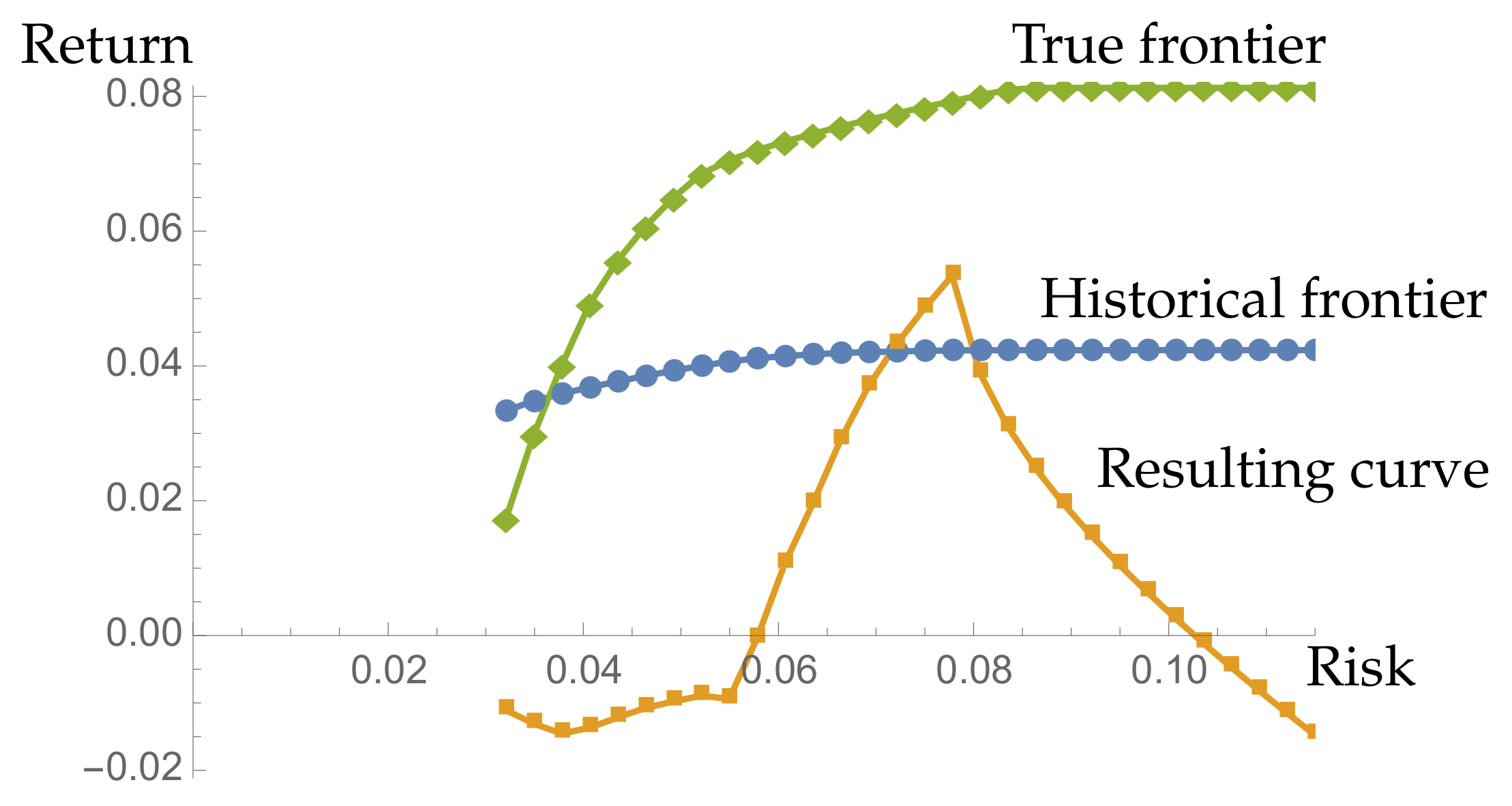
Now let be the vector of historical returns provided by the n assets in the -th period and, for each level of risk R, let be the true return provided by the efficient portfolio corresponding to R in the -th period. The set of pairs form the so called resulting curve (which, of course, is only known a posteriori).
On the other hand, for each level of risk R, we solve the portfolio selection problem with instead of in the objective function. The pairs give rise to the true efficient frontier, which indicates the return we could have obtained if we had known a priori the returns of the -th period.
Figure 1 illustrates these concepts. The value of information for a given level of risk is the difference between the “true return” obtained from the true returns on the assets minus the resulting return. It represents the money the investor would have obtained if he had known a priori the true returns of the assets.
In [
22], we use the value of information to define an index measuring the financial impact of each possible set of diversification constraints when it is incorporated into a portfolio selection model, but, to this purpose, the above defined value of information has an obvious drawback, namely, that it takes as ideal reference an exact forecasting of the return of each asset, and hence the index defined in [
22] does not take into account the possible effects that a good—but not exact—forecast would produce. This is not important in order to establish a relative ranking of several alternative sets of diversification constraints, as we did in [
22], but in order to select the most adequate one in a particular context, it is desirable to somehow include into our analysis the reliability of the forecasted returns the investor is considering. Thus, in the next section we revisit the reduction index introduced in [
22].
3. The Historical Reduction Index of a Set of Diversification Constraints
Consider an investor wishing to select a portfolio from a set of n possible assets by using a given vector of forecasted returns. If the forecast comes from non-statistical sources (expert opinions, ad hoc information about the market, etc.) the main problem is that in this context we do not have any statistical measure of the risk of any possible portfolio. The risk is very related with the reliability of the forecasting, since, as we have commented, if the investor could be sure that the forecasted values are exact, risk would be null, and the best investment policy would be putting all the available capital in the asset with greater forecasted return. This means investing with no diversification. Of course, this will never happen in the real world, and the less reliable the forecast is, the more diversification should be introduced in the selection criterion. But, how can we determine how much diversification is desirable? How can we quantify “the diversification” of a portfolio?
In short, our proposal consists of simulating forecasts with a given degree of reliability from the historical returns of the assets and measuring the financial impact of a given set of diversification constraints. First, we precise the idea of “degree of reliability”.
Consider a set of n assets whose historical returns are known in T consecutive periods (the T-th period corresponding to the time at which the investment is to be decided). Let be the historical return of the i-th asset in the k-th period.
We fix a length t for a rolling window, which will vary from the period t to the period . This means that we consider the mean return for the i-th asset at period k defined as the mean of the historical returns . Similarly, the covariance matrix is defined as the covariance matrix of the historical returns in the same t periods.
A simulated forecast for n assets at the k-th period with reliability will be a (computer generated) random variate of a normal distribution , where is the (sample) standard deviation of the historical returns provided by the i-th asset from period to k. We also consider as the only “simulated forecast” with reliability the one consisting of the returns .
Thus, a “simulated forecast” of reliability is the exact forecast consisting of the true returns provided by each asset in the -th period, whereas a simulated forecast of reliability is the result of a (pseudo)-random experiment corresponding to a random variable with mean (the true return of the next period) and standard deviation varying from the historical one (corresponding to ) to 0 (as tends to 1).
In this approach, we are conceiving forecasts as measures of objective values (the returns of the next investment period) subjected to measurement errors, and we deal with those errors in the standard way, namely, by means of a normal distribution.
Now, following [
22], we fix a historical base portfolio selection problem (HP
) that maximizes the expected return at the
k-th period (calculated as
) subject to the capital constraint
and any other constraint considered by the investor not related to risk aversion. The simplest possibility is:
If S is a set of diversification constraints, let HP be the problem consisting of HP plus the constraints in S. Let be the set of diversification constraints that the investor would consider adequate if they would be willing to use the historical means as expected returns. For instance, if we take the simplest version of HP and , where is a given level of admissible risk, then HP is the classical Markowitz problem.
For a simulated forecast corresponding to the k-th period, the forecasting problem FP (resp. FP) is defined as the problem obtained by changing the objective function of HP (resp. HP) from to .
If is the optimal solution of a problem HP, HP or FP, we define the true return of the corresponding problem as , i.e., the return that portfolio provides at period .
Now, for a fixed , we define the historical reduction index associated to and to a set S of diversification constraints with regard to a base set of diversification constraints as the real number calculated with the following procedure:
Step 1 Generate a large number N of simulated forecasts at the k-th period with reliability for .
Step 2 Calculate the true return of the problem FP, the true return of the problem FP and the true return of the problem HP.
Step 3 Compute the
absolute and the
relative mean true returns Step 4 Compute the
absolute and the
relative value of each forecast as:
Step 5 Compute the
mean absolute and
relative value of the forecasts as
Step 6 Calculate the historical reduction index as
The definition for is the same, except that in the first step there is just one simulated forecast and hence no average is calculated in Step 3. The interpretation of the concepts we have introduced is clear:
and are the mean returns provided by the portfolio selected from a forecast with reliability with no diversification constraint or with the set S of diversification constraints, respectively, at period k.
and
are the net profit provided by a forecast with reliability
with regard to the profit attained when the historical mean returns are taken as expected returns (they generalize the concept of value of information of [
22], which in turn generalize that of [
15]).
and are the mean value of a forecast of reliability in the period under consideration (without diversification constraints and with those in the set S, respectively).
The quotient represents the percentage of profit that is preserved after imposing the set S of diversification constraints, and hence is the percentage in which the constraints S reduce the profit.
4. Empirical Analysis of the Behavior of the Index
We have considered the monthly historical returns of 30 assets (those identified by the tickers ABE, ANA, ACS, AMS, BBVA, SAB, SAN, BKT, BME, CABK, DIA, ENG, ELE, FER, FCC, GAM, GAS, GRF, IBE, IDR, ITX, IAG, JAZ, MAP, TL5, OHL REE, REP, TRE, and TEF.) from the Spanish IBEX35 index in the period ranging from August 2011 to July 2015 (we have chosen those included in the index through the whole period). More specifically, we have considered a rolling window giving rise to 12 data sets corresponding to each month from August 2014 to July 2015 with the expected returns and the covariance matrix calculated from the previous 36 months.
We set as a base problem:
and take
. We have computed HRI
for several sets of constraints by using a set of 50 simulated forecasts for each period and each level of reliability
.
The first family of sets of diversification constraints that we have considered are those based in bounding the standard deviation of the expected return of the portfolio based on the historical data, namely:
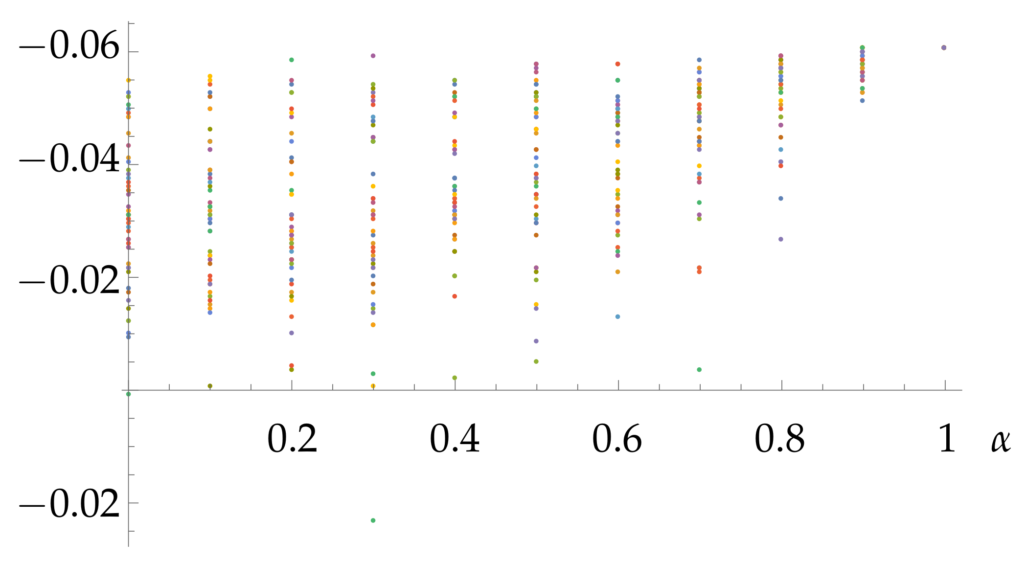
Figure 2 shows the true returns provided by the 50 simulated forecasts for each level of reliability
in the first period (August 2014) for the set
. Notice that they are bounded by the single true return corresponding to
, since no forecast can provide a better true return than the exact one.
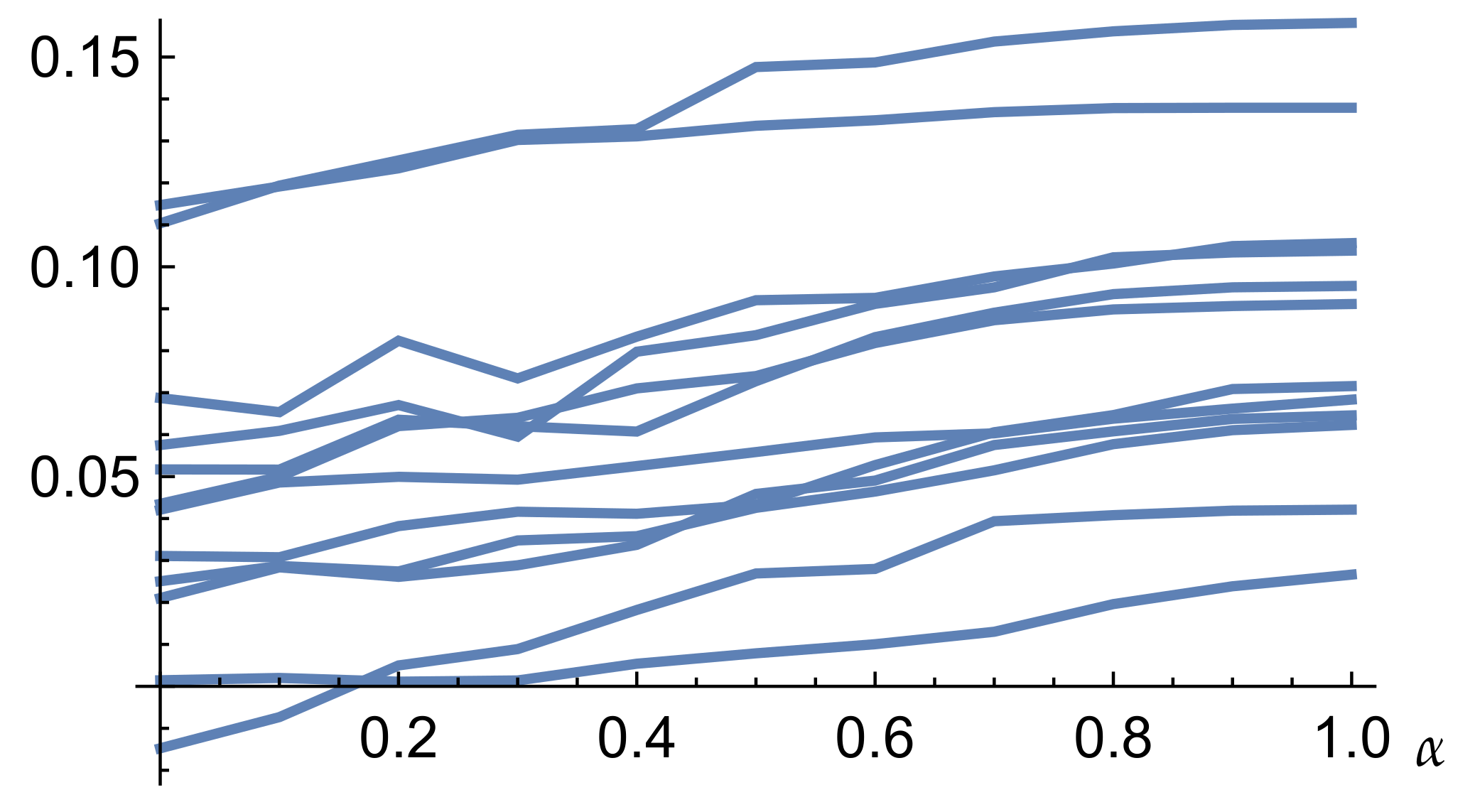
Figure 3 shows the relative value
for each period
k. Notice that the data contained in
Figure 2 determine a single curve in
Figure 3, namely, that taking the least value at
. It is calculated as the average of the corresponding values shown in
Figure 2 minus the true return provided by HP
, which in this case is
.
To that extent, we are facing the unpredictable nature of portfolio selection (of course, for a particular case, not in the statistical sense): different simulated forecasts with the same reliability provide quite different true returns and the relative (mean) value of a forecast with reliability can be quite different at each period. Even some of them (for lower levels of reliability) can provide worse true returns than the selection criterion based on the historical data.
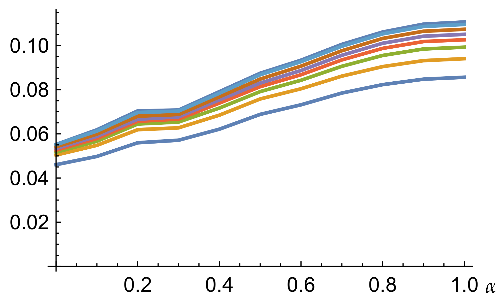
However,
Figure 4 shows that these irregular data are hiding a quite regular pattern. The bottom-most curve in this figure is the average of the curves shown in
Figure 3, i.e., the curve
. As the risk constraint is weakened, i.e., as we consider the constraint sets
, for greater values of
j, we obtain a strictly increasing sequence of curves approaching the top-most one, which is the absolute value
of the simulated forecasts of level
.
We can see that, with a conservative risk constraint , the true return can exceed the one provided by the selection based in the historical data in an amount ranging from for to for . This difference increases as the risk constraint is weakened. We say that is a conservative level of risk because we are assuming that this is the level of risk that the investor considers adequate for selecting a portfolio with the expected returns provided by the historical data, and one can assume that an investor who considers quite reliable a given forecast should accept a greater level of risk when selecting a portfolio from his forecast than just from the historical data.
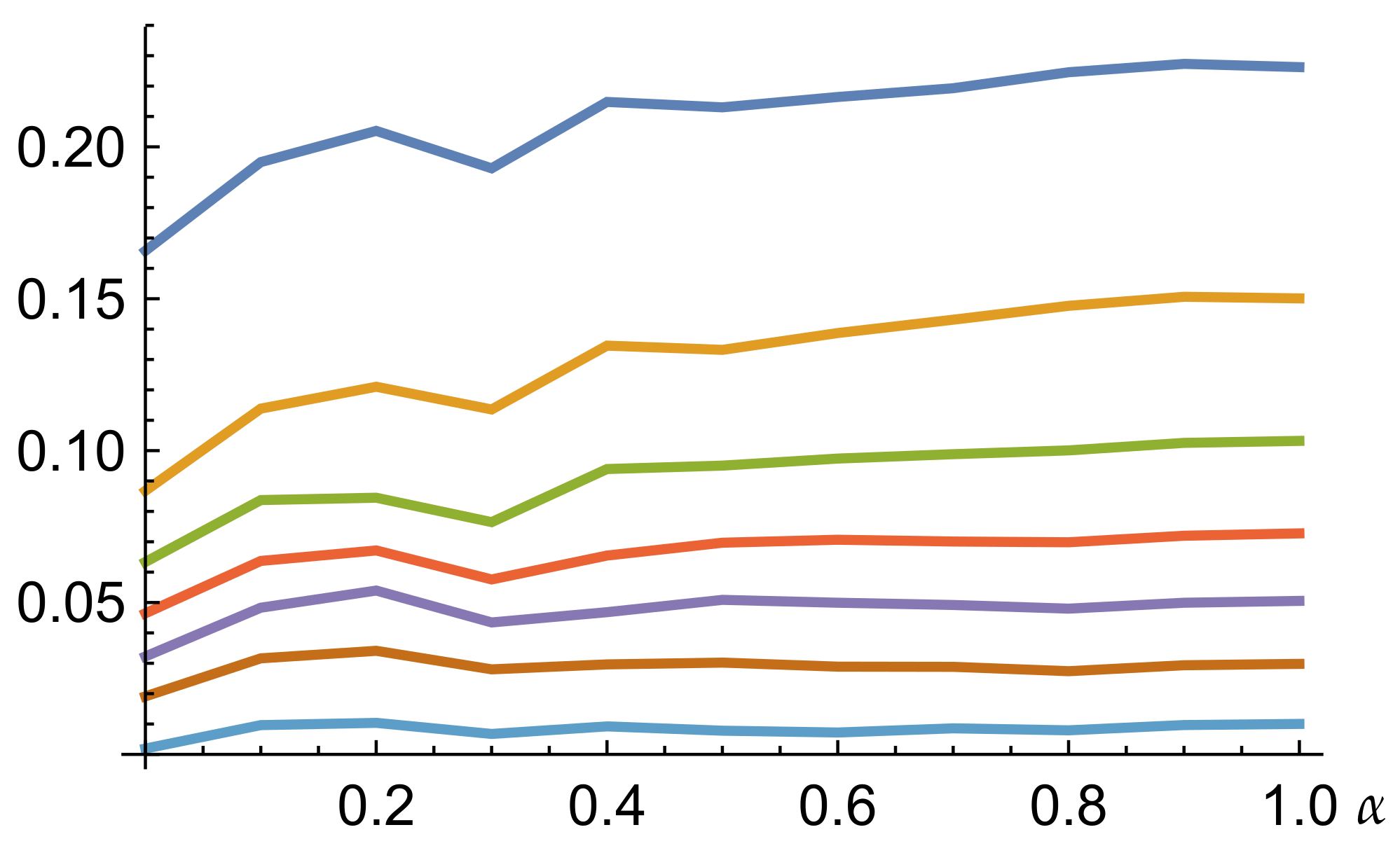
Finally,
Figure 5 shows the historical reduction index of the sets
for each
j and
. Again the curves are strictly monotonic: the higher
j, the lower curve. We remark again that the regularity shown in
Figure 4 and
Figure 5 reveal that the means we have taken to calculate them make sense: from a random set of values, one can always take their mean for obtaining a single value, but if the means we have taken had not an intrinsic meaning, the curves in
Figure 4 and
Figure 5 would be expected to intersect themselves randomly instead of exhibiting such a regular pattern. Hence, we get a strict grading of the considered sets of diversification constraints that is independent of
. Thus, we conclude that the index HRI
contains sound financial information about the set
S.
Notice also that each curve in
Figure 5 is quite chaotic for small levels of reliability, but stabilizes for
, becoming quite insensitive to the specific level of reliability fixed by the investor. This plays down the importance of obtaining a precise estimate of this level.
Table 1 contains the values plotted in
Figure 5.
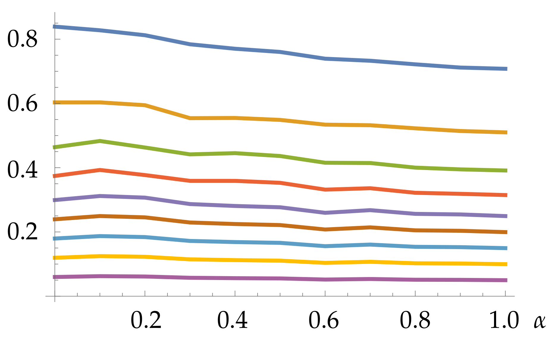
Consider now the sets of diversification constraints consisting of imposing an upper bound to each weight, namely:
Figure 6 shows the corresponding historical reduction index. We see again a strictly regular pattern providing a grading of the diversification constraints: the greater bounds, the less reduction index, but we should emphasize that this seemingly obvious relation only holds in the average, since for each particular forecast and each particular period we obtain graphs as irregular as those in
Figure 2 and
Figure 3.
Table 2 contains the values shown in
Figure 6.
We observe that the reduction index for upper bounds on the weights are even less sensitive to the level of reliability than that for bounds on the standard deviation. On the other hand, considering, for instance
, we see that the impact of an upper bound
is quite stronger than
(the HRI changes from a
to a
, much more than the next step, which leads to a
). But the most remarkable fact is that now we can compare the impact of the two types of diversification constraints. For instance,
Table 3 contains the historical reduction index for
corresponding to the upper bounds on the weights and on the standard deviation. We see that upper bounds on the weights less than
are stronger than all the risk constraints we are considering, whereas
is almost equivalent to
. It should be remarked that those comparisons heavily depend on the total number of considered assets.
In the same way, any other set of diversification constraints can be compared with those we have considered by means of the HRI, including, for instance, simultaneous bounds on the weight and on the standard deviation.
5. Conclusions
In this paper we have considered the problem derived from the inclusion of additional non-historical information in the forecasting of the expected returns of financial assets, in portfolio selection problems. We have introduced an index measuring the impact of each possible set of diversification constraints depending on a parameter estimating the subjective reliability of the forecast. Our empirical analysis shows that the index is suitable for the purpose it has been designed for. Namely:
The reduction index is sound, in the sense that it reveals an absolute grading between different possible sets of diversification constraints which gives the investor a clear picture of which sets of constraints are more or less constraining, even if they are of very different nature.
It is robust, in the sense that, as we have seen, the gradings it produces are only a little sensitive to the precise value of
(which could be hard to determine with accuracy because of its highly subjective nature). Incidentally, this justifies that the analysis done by Kao and Steuer [
15] is not unrealistic for having considered exact forecasts, since the results having considered enough reliable ones would have been the same.
It is very versatile, since it does not depend on the nature of the considered diversification constraints, and hence the proposed technique for grading and selecting alternative sets of constraints can be applied to any kind of such constraints.
However, at the same time, it is rather specific, since it adjusts to each set of assets under consideration and each specific considered date since it takes into account the previous historical information about the returns provided by the assets.
Author Contributions
Conceptualization, C.C., C.I., V.L. and B.P.-G.; methodology, C.C., C.I., V.L. and B.P.-G.; software, C.C., C.I., V.L. and B.P.-G.; validation, C.C., C.I., V.L. and B.P.-G.; formal analysis, C.C., C.I., V.L. and B.P.-G.; investigation, C.C., C.I., V.L. and B.P.-G.; resources, C.C., C.I., V.L. and B.P.-G.; data curation, C.C., C.I., V.L. and B.P.-G.; writing—original draft preparation, C.C., C.I., V.L. and B.P.-G.; writing—review and editing, C.C., C.I., V.L. and B.P.-G.; visualization, C.C., C.I., V.L. and B.P.-G.; supervision, C.C., C.I., V.L. and B.P.-G.; project administration, C.C., C.I., V.L. and B.P.-G.; funding acquisition, C.C., C.I., V.L. and B.P.-G. All authors have read and agreed to the published version of the manuscript.
Funding
This work has been supported by the Spanish Ministerio de Ciencia, Innovación y Universidades, project reference number: RTI2018-093541-B-I00.
Institutional Review Board Statement
Not applicable.
Informed Consent Statement
Not applicable.
Data Availability Statement
The data presented in this study are available on request from the corresponding author.
Conflicts of Interest
The authors declare no conflict of interest. The funders had no role in the design of the study; in the collection, analyses, or interpretation of data; in the writing of the manuscript, or in the decision to publish the results.
References
- Markowitz, H.M. Portfolio selection. J. Financ. 1952, 7, 77–91. [Google Scholar]
- Markowitz, H.M. Portfolio Selection: Efficient Diversification of Investments; John Wiley: New York, NY, USA, 1959. [Google Scholar]
- Aouni, B.; Doumpos, M.; Pérez-Gladish, B.; Steuer, R.E. On the increasing importance of multiple criteria decision aid methods for portfolio selection. J. Oper. Res. Soc. 2018, 69, 1525–1542. [Google Scholar] [CrossRef]
- Low, R.K.Y.; Faff, R.; Aas, K. Enhancing mean-variance portfolio selection by modeling distributional asymmetries. J. Econ. Bus. 2016, 85, 49–72. [Google Scholar] [CrossRef] [Green Version]
- Artzner, P.; Delbaen, F.; Eber, J.M.; Heath, D. Coherent Measures of Risk. Math. Financ. 1999, 9, 203–228. [Google Scholar] [CrossRef]
- Doganoglu, T.; Hartz, C.; Mittnik, S. Portfolio Optimization When Risk Factors Are Conditionally Varying and Heavy Tailed. Comput. Econ. 2007, 29, 333–354. [Google Scholar] [CrossRef] [Green Version]
- Rachev, S.T.; Mittnik, S. Stable Paretian Models in Finance; Wiley: New York, NY, USA, 2000; ISBN 978-0-471-95314-2. [Google Scholar]
- Taleb, N.N. The Black Swan: The Impact of the Highly Improbable; Random House: New York, NY, USA, 2007; ISBN 978-1-4000-6351-2. [Google Scholar]
- Rom, B.M.; Ferguson, K.W. Post-Modern Portfolio Theory Comes of Age. J. Invest. 1994, 1, 349–364. [Google Scholar] [CrossRef]
- Rom, B.M.; Ferguson, K. A software developer’s view: Using Post-Modern Portfolio Theory to improve investment performance measurement. In Managing Downside Risk in Financial Markets: Theory, Practice and Implementation; Sortino, F.A., Satchell, S., Eds.; Butterworth-Heinemann Finance: Oxford, UK, 2001; p. 59. [Google Scholar]
- Campbell, J.Y.; Lo, A.W.; MacKinlay, A.C. The Econometrics of Financial Markets; Princeton University Press: New Jersey, NY, USA, 1996. [Google Scholar]
- Kingdon, J. Intelligent Systems and Financial Forecasting; Springer: Berlin, Germany, 1997. [Google Scholar]
- Bettner, M.S. Using Accounting & Financial Information. Analyzing, Forecasting & Decision Making; Bussines Expert Press: New York, NY, USA, 2015. [Google Scholar]
- Plummer, T. Forecasting Financial Markets. The Psychology of Successful Investing; Kogan Page: London, UK, 2010. [Google Scholar]
- Kao, C.; Steuer, R.E. Value of information in portfolio selection, with a Taiwan stock market application illustration. Eur. J. Oper. Res. 2016, 253, 418–427. [Google Scholar] [CrossRef]
- Chopra, V.K.; Ziemba, W.T. The effect of errors in means, variances, and covariances on optimal portfolio choice. J. Portfolio Manag. 1993, 19, 6–11. [Google Scholar] [CrossRef]
- Best, M.J.; Grauer, R.R. On the sensitivity of mean–variance-efficient port- folios to changes in asset means: Some analytical and computational results. Rev. Financ. Stud. 1991, 4, 315–342. [Google Scholar] [CrossRef] [Green Version]
- DeMiguel, V.; Nogales, F.J. Portfolio selection with robust estimation. Oper. Res. 2009, 57, 560–577. [Google Scholar] [CrossRef]
- Kan, R.; Smith, D.R. The distribution of the sample minimum-variance frontier. Manag. Sci. 2008, 54, 1364–1380. [Google Scholar] [CrossRef] [Green Version]
- Siegal, A.F.; Woodgate, A. Performance of portfolios optimized with estimation error. Manag. Sci. 2007, 53, 1005–1015. [Google Scholar] [CrossRef] [Green Version]
- Copeland, T.E.; Weston, J.F. Financial Theory and Corporate Policy; Addison-Wesley: Reading, MA, USA, 1983. [Google Scholar]
- Calvo, C.; Ivorra, C.; Liern, V. Controlling risk through diversification in portfolio selection with non-historical information. J. Oper. Res. Soc. 2017. [Google Scholar] [CrossRef]
| Publisher’s Note: MDPI stays neutral with regard to jurisdictional claims in published maps and institutional affiliations. |
© 2021 by the authors. Licensee MDPI, Basel, Switzerland. This article is an open access article distributed under the terms and conditions of the Creative Commons Attribution (CC BY) license (http://creativecommons.org/licenses/by/4.0/).


