Fuzzy Numerical Solution via Finite Difference Scheme of Wave Equation in Double Parametrical Fuzzy Number Form

Abstract

The use of fuzzy partial differential equations has become an important tool in which uncertainty or vagueness exists to model real-life problems. In this article, two numerical techniques based on finite difference schemes that are the centered time center space and implicit schemes to solve fuzzy wave equations were used. The core of the article is to formulate a new form of centered time center space and implicit schemes to obtain numerical solutions fuzzy wave equations in the double parametric fuzzy number approach. Convex normalized triangular fuzzy numbers are represented by fuzziness, based on a double parametric fuzzy number form. The properties of fuzzy set theory are used for the fuzzy analysis and formulation of the proposed numerical schemes followed by the new proof stability thermos under in the double parametric form of fuzzy numbers approach. The consistency and the convergence of the proposed scheme are discussed. Two test examples are carried out to illustrate the feasibility of the numerical schemes and the new results are displayed in the forms of tables and figures where the results show that the schemes have not only been effective for accuracy but also for reducing computational cost.

1. Introduction

One of the effective ways of modelling ambiguity and imprecision in certain quantities for certain real-life problems are fuzzy partial differential equations (FPDEs). FPDEs were recently utilised in a number of areas, including physics, biology, chemistry and engineering [1,2,3,4,5].

The analytical solution of the PDEs is often impractical to obtain due to the complexity of the model. So, there is increasing interest in obtaining numerical solutions using numerical methods. The finite difference methods are some of the important forms of numerical methods. These methods have been used by many mathematicians for solving FPDEs. Nemati and Matinfar [6] developed an implicit finite difference scheme for solving some fuzzy partial differential equations. The stability analysis of the proposed implicit scheme was studied. Numerical experiments involving parabolic partial differential equations were presented to illustrate the capability and feasibility of the proposed method. An explicit numerical solution of fuzzy hyperbolic and parabolic equations was presented by Allahviranloo and Kermani [7]. The existence and stability of the presented scheme were examined to show that the scheme is conditionally stable. Two numerical examples were presented to illustrate the capability of the proposed scheme. The FTCS also was applied by Zureigat and Izani [8] to obtain a numerical solution for fuzzy heat equations under two different types of fuzzifications. The effect on the numerical solutions for both types of fuzzifications was discussed. It was found that the solution of the fuzzy heat equation with a small fuzzy number area provides more accurate results than the large area. Abdi and Allahviranloo [9] implemented the finite difference method to solve the fuzzy Poisson’s equation with Dirichlet boundary conditions. The convergence of the proposed method was investigated and a numerical example was solved for more illustration of the proposed approach.

A second-order FPDE for the explanation of such a wave equation involving uncertainty is the fuzzy wave equation (FEW). It may be present in the areas of electromagnetism, acoustics and fluid dynamics [10,11,12,13,14]. Some authors have recently researched the FWE approximate and numerical solutions in the single parametric form of fuzzy numbers. In solving FWEs in one and two dimensions, Allaahviranloo et. al and Chadil et al. used the variational iteration method (VIM) in [15,16] and it was found that the approach to solving FWEs is very efficient and easy. Moreover, the presented method was found to be convenient, clear and straightforward for the approximation of the successive approach. Hashemi and Malekinagad used the homotopy analysis method (HAM) to solve some FPDEs which were classified as an approximate analytical method that can be used to obtain a series solutions of different types of linear and nonlinear equations. It was found that the HAM is a promising tool for solving FWEs [17]. For the numerical solution of initial boundary value problems involving FWEs, Aylin Bayrak suggested and analyzed a numerical approach based on the finite difference methods which showed accuracy and capability [18].

The n × n fuzzy differential equation system is transformed from a single parametric form of a fuzzy number in the 2n × 2n crisp differential equation system. The n × n fuzzy differential equation system is transformed to a crisp system of the same order for the double parameter form of a fuzzy number. This approach has been proposed to solve fuzzy fractional parabolic partial differential equations under the double parameter form of a fuzzy number by utilizing a single parametric form of fuzzy numbers to convert the FPDEs into an interval-based fuzzy partial differential equation via an implicit finite difference scheme [19]. The double parametric form technique has been discovered to be general and not complicated and requires less calculation than the single form.

From the above literature, the obtained results show that some research was conducted with approximate and numerical methods that also involved finite difference schemes for solving FWEs in single parameter form. Therefore, the aim of this work is to reformulate the standard finite difference methods to obtain new forms of the cantered time centre space and implicit schemes and prove the stability thermos for the numerical solution of the FWE under the double parametric form of fuzzy numbers for the first time. We would also like to point out that this paper focuses on computational and formal issues; discussion can also be retrieved in [20] on the physical significance of fading solutions to partial differential equations.

This work is organized as follows—in Section 2 the fuzzy wave equation with necessary fuzzy analysis on double parametric form of fuzzy number details is recalled. A description of the centre time centre space (CTCS) scheme formula for solving a fuzzy wave equation is given in Section 3. Section 4 is focused on the implicit scheme to obtain a numerical solution of a fuzzy wave equation followed by fuzzy stability analysis and theorem for the CTCS scheme in Section 5. In Section 6, two numerical examples are presented to show the method efficiency under a new approach to the fuzzy number. Finally, there is a short summary of this work. It should be noted that some of the fuzzy sets concepts and definitions not given in this work are standard. Notions of fuzzy level sets, fuzzy numbers, fuzzy functions, fuzzy Zadeh expansion theory and fuzzy H-derivatives can be checked from the literature, e.g., [20,21,22,23,24].

2. The FEW in General From

Consider the FWE with the indicated initial conditions [15]:

$$\frac{{\partial }^2\tilde{u}\left(x,t\right)}{\partial t^2}=\tilde{D}\frac{{\partial }^2\tilde{u}\left(x,t\right)}{\partial x^2}+\tilde{g}\left(x\right), 0<x<l, t>0$$

(1)

$$\tilde{u}\left(x,0\right)=\widetilde{f_1}\left(x\right),\frac{\partial u}{\partial t}\left(x,0\right)={\tilde{f}}_2\left(x\right),\tilde{u}\left(0,t\right)=\tilde{v},\tilde{u}\left(l,0\right)=\tilde{y},$$

where $\tilde{u}\left(t,x\right)$ is the fuzzy function of the crisp independent variables $t$ and x and the nonhomogeneous term $\tilde{g}\left(x\right)$ is a fuzzy function of crisp variable $x$. The $\frac{{\partial }^2\tilde{u}\left(x,t\right)}{\partial t^2} \mathrm{and} \frac{{\partial }^2\tilde{u}\left(x,t\right)}{\partial x^2}$ are the second order fuzzy partial generalized derivatives [25]. Furthermore, in Equation (1) the fuzzy initial conditions are $\tilde{u}\left(0,x\right)$, $\frac{\partial u}{\partial t}\left(x,0\right)$ and ${\tilde{f}}_1\left(x\right)$ and ${\tilde{f}}_2\left(x\right)$ are fuzzy functions of $x$.The boundary conditions in fuzzy form are $\tilde{u}\left(0,t\right)$ and $\tilde{u}\left(l,0\right)$ and are equal to the fuzzy convex numbers $\tilde{v}$ and $\tilde{y},$ respectively.

The FWE in this section is defuzzified via the double parametric approach of fuzzy number as presented in [18]. We may write Equation (1) in single parametric form of the fuzzy number. The following may be written:

The generalized differentiability which is used in this paper is defined as follows [25,26]:

Let be $\mathrm{F}:\mathrm{a},\mathrm{b}\to {\mathrm{F}}^{\mathrm{n}}$ and ${\mathrm{t}}_0ϵ\left(\mathrm{a},\mathrm{b}\right)$, we say that F is differentiable at ${\mathrm{t}}_0$ if:

(1)

It exists an element ${\mathrm{f}}^{\prime }({\mathrm{t}}_0) ϵ{\mathrm{F}}^{\mathrm{n}}$ such that, for all $\mathrm{h}>0$ sufficiently near to 0, there are $\mathrm{F}\left({\mathrm{t}}_0+\mathrm{h}\right)-\mathrm{F}\left({\mathrm{t}}_0\right),\mathrm{F}\left({\mathrm{t}}_0\right)-\mathrm{F}\left({\mathrm{t}}_0-\mathrm{h}\right)$ and the limit

$$\underset{\mathrm{h}\to 0+}{\lim } \frac{\mathrm{F}\left({\mathrm{t}}_0+\mathrm{h}\right)-\mathrm{F}\left({\mathrm{t}}_0\right)}{\mathrm{h}}=\underset{\mathrm{h}\to 0+}{\lim }\frac{\mathrm{F}\left({\mathrm{t}}_0\right)-\mathrm{F}\left({\mathrm{t}}_0-\mathrm{h}\right)}{\mathrm{h}}= {\mathrm{F}}^{\prime }({\mathrm{t}}_0)$$

or

(2)

It exists an element ${\mathrm{f}}^{\prime }({\mathrm{t}}_0) ϵ{\mathrm{F}}^{\mathrm{n}}$ such that, for all $\mathrm{h}<0$ sufficiently near to 0, there are $\mathrm{F}\left({\mathrm{t}}_0+\mathrm{h}\right)-\mathrm{F}\left({\mathrm{t}}_0\right),\mathrm{F}\left({\mathrm{t}}_0\right)-\mathrm{F}\left({\mathrm{t}}_0-\mathrm{h}\right)$ and the limit

$$\underset{\mathrm{h}\to 0-}{\lim } \frac{\mathrm{F}\left({\mathrm{t}}_0+\mathrm{h}\right)-\mathrm{F}\left({\mathrm{t}}_0\right)}{\mathrm{h}}=\underset{\mathrm{h}\to 0-}{\lim }\frac{\mathrm{F}\left({\mathrm{t}}_0\right)-\mathrm{F}\left({\mathrm{t}}_0-\mathrm{h}\right)}{\mathrm{h}}= {\mathrm{F}}^{\prime }({\mathrm{t}}_0)$$

(2)

Based on the generalized differentiability that are defined in [25,26] there are four cases that we can classify into two cases, the first case by definition of standard difference that the following equations must hold:

First case: by definition of standard difference that the following equations must hold

$$\left[\frac{{\partial }^2\underset{\_}{u}\left(x,t,\beta ;r\right)}{\partial t^2}, \frac{{\partial }^2\overline{u}\left(x,t,\beta ;r\right)}{\partial t^2}\right]=\left[ \underset{\_}{D}\left(x,r\right),\overline{D}\left(x,r\right)\right]\left[\frac{{\partial }^2{\underset{\_}{u}}_{i,n}\left(x,t;r\right)}{\partial x^2},\frac{{\partial }^2{\overline{u}}_{i,n}\left(x,t;r\right)}{\partial x^2}\right]+\left[\underset{\_}{g}\left(x,t;r\right),\overline{g}\left(x,t;r\right)\right],$$

(3)

subjected to the fuzzy initial and boundary conditions

$$\{\begin{array}{c}\left[\underset{\_}{u}\left(x,t;r,\beta \right),\overline{u}\left(x,t;r,\beta \right)\right]=\left[\underset{\_}{f_1}\left(x,t;r,\beta \right),\overline{f_1}\left(x,t;r,\beta \right)\right],\\ \left[\underset{\_}{u_t}\left(x,t;r,\beta \right),\overline{u_t}\left(x,t;r,\beta \right)\right]=[\underset{\_}{f_2}\left(x,t;\beta ,r\right),\overline{f_2}\left(x,t;r,\beta \right),\\ \left[\underset{\_}{u}\left(0,t;r,\beta \right),\overline{u}\left(0,t;r,\beta \right)\right]=\left[\underset{\_}{v}\left(0,t;r,\beta \right),\overline{v}\left(0,t;r,\beta \right)\right],\\ \left[\underset{\_}{u}\left(l,t;r,\beta \right),\overline{u}\left(l,t;r,\beta \right)\right]=\left[\underset{\_}{y}\left(l,t;r,\beta \right),\overline{y}\left(l,t;r,\beta \right)\right].\end{array}$$

Now, according to the definition of fuzzy double parametric in [19], Equation (3) is as follows:

$$\begin{array}{ll}\{\beta (\frac{{\partial }^2\overline{u}\left(x,t;\beta ,r\right)}{\partial t^2}& -\frac{{\partial }^2\underset{\_}{u}\left(x,t;\beta ,r\right)}{\partial t^2})+\frac{{\partial }^2\underset{\_}{u}\left(x,t;\beta ,r\right)}{\partial t^2}\}\\ & =\left\{\beta \left(\overline{D}\left(x;r\right)-\underset{\_}{D}\left(x;r\right)\right)+\underset{\_}{D}\left(x;r\right)\right\}\left\{\beta \left(\frac{{\partial }^2{\overline{u}}_{i,n}\left(x,t;r\right)}{\partial x^2}-\frac{{\partial }^2{\underset{\_}{u}}_{i,n}\left(x,t;r\right)}{\partial x^2}\right)+\frac{{\partial }^2{\underset{\_}{u}}_{i,n}\left(x,t;r\right)}{\partial x^2}\right\}\\ & +\left\{\beta \left(\overline{g}\left(x,t;r\right)-\underset{\_}{g}\left(x,t;r\right)\right)+\underset{\_}{g}\left(x,t;r\right)\right\},\end{array}$$

(4)

subjected to the fuzzy initial and boundary conditions

$$\begin{array}{l}\{\beta \left(\overline{u}\left(x,0;r\right)-\underset{\_}{u}\left(x,0;r\right)\right)+\underset{\_}{u}\left(x,0;r\right)\}=\left\{\beta \left(\overline{f_1}\left(x,r\right)-\underset{\_}{f_1}\left(x,r\right)\right)+\underset{\_}{f_1}\left(x,r\right)\right\},\\ \{\beta \left(\overline{u_t}\left(x,0;r\right)-\underset{\_}{u_t}\left(x,0;r\right)\right)+\underset{\_}{u_t}\left(x,0;r\right)\}=\left\{\beta \left(\overline{f_2}\left(x,r\right)-\underset{\_}{f_2}\left(x,r\right)\right)+\underset{\_}{f_2}\left(x,r\right)\right\},\\ \{\beta \left(\overline{u}\left(0,t;r\right)-\underset{\_}{u}\left(0,t;r\right)\right)+\underset{\_}{u}\left(0,t;r\right)\}=\left\{\beta \left(\overline{v}\left(x,r\right)-\underset{\_}{v}\left(x,r\right)\right)+\underset{\_}{v}\left(x,r\right)\right\},\\ \{\beta \left(\overline{u}\left(1,t;r\right)-\underset{\_}{u}\left(1,t;r\right)\right)+\underset{\_}{u}\left(1,t;r\right)\}=\left\{\beta \left(\overline{y}\left(x,r\right)-\underset{\_}{y}\left(x,r\right)\right)+\underset{\_}{y}\left(x,r\right)\right\},\end{array}$$

where $\beta \in \left[0,1\right]$. Now we write:

$$\begin{gathered} \frac{{\partial }^2\tilde{u}\left(x,t;\beta ,r\right)}{\partial t^2}=\left\{\beta \left(\frac{{\partial }^2\overline{u}\left(x,t,\alpha ;r\right)}{\partial t^2}-\frac{{\partial }^2\underset{\_}{u}\left(x,t,\alpha ;r\right)}{\partial t^2}\right)+\frac{{\partial }^2\underset{\_}{u}\left(x,t,\alpha ;r\right)}{\partial t^2}\right\}, \\ \tilde{D}\left(x\right)\frac{{\partial }^2\tilde{u}\left(x,t;\beta ,r\right)}{\partial x^2}=\left\{\beta \left(\overline{D}\left(x;r\right)-\underset{\_}{D}\left(x;r\right)\right)+\underset{\_}{D}\left(x;r\right)\right\}\left\{\beta \left(\frac{{\partial }^2{\overline{u}}_{i,n}\left(x,t;r\right)}{\partial x^2}-\frac{{\partial }^2{\underset{\_}{u}}_{i,n}\left(x,t;r\right)}{\partial x^2}\right)+\frac{{\partial }^2{\underset{\_}{u}}_{i,n}\left(x,t;r\right)}{\partial x^2}\right\}, \\ \tilde{g}\left(x,t;\beta ,r\right)=\left\{\beta \left(\overline{g}\left(x,t;r\right)-\underset{\_}{g}\left(x,t;r\right)\right)+\underset{\_}{g}\left(x,t;r\right)\right\}, \\ \tilde{u}\left(x,0;\beta ,r\right)=\left\{\beta \left(\overline{u}\left(x,0;r\right)-\underset{\_}{u}\left(x,0;r\right)\right)+\underset{\_}{u}\left(x,0;r\right)\right\}, \\ \tilde{f}\left(x;\beta ,r\right)=\left\{\beta \left(\overline{f}\left(x;r\right)-\underset{\_}{f}\left(x;r\right)\right)+\underset{\_}{f}\left(x;r\right)\right\}, \\ \tilde{u}\left(0,t;\beta ,r\right)=\left\{\beta \left(\overline{u}\left(0,t;r\right)-\underset{\_}{u}\left(0,t;r\right)\right)+\underset{\_}{u}\left(0,t;r\right)\right\}, \\ \tilde{g}\left(x,;\beta ,r\right)=\left\{\beta \left(\overline{v}\left(x;r\right)-\underset{\_}{v}\left(x;r\right)\right)+\underset{\_}{v}\left(x;r\right)\right\}, \\ \tilde{u}\left(1,t,;\beta ,r\right)=\left\{\beta \left(\overline{u}\left(1,t;r\right)-\underset{\_}{u}\left(1,t;r\right)\right)+\underset{\_}{u}\left(1,t;r\right)\right\}, \\ \tilde{y}\left(x;\beta ,r\right)=\left\{\beta \left(\overline{y}\left(x;r\right)-\underset{\_}{y}\left(x;r\right)\right)+\underset{\_}{y}\left(x;r\right)\right\}. \end{gathered}$$

Substituting these into Equation (1) gives:

$$\begin{gathered} \frac{{\partial }^2\tilde{u}\left(x,t;r,\beta \right)}{\partial t^2}=\tilde{D}\left(x\right)\frac{{\partial }^2\tilde{u}\left(x,t;r,\beta \right)}{\partial x^2}+\tilde{g}\left(x,t,\beta \right), 0<x<l, t>0 \\ \tilde{u}\left(x,0,\beta \right)=\widetilde{f_1}\left(x,r,\beta \right), \frac{\partial u}{\partial t}\left(x,0,\beta \right)={\tilde{f}}_2\left(x,r,\beta \right),\tilde{u}\left(0,t,\beta \right)=\tilde{v}, \tilde{u}\left(l,t,\beta \right)=\tilde{y}. \end{gathered}$$

(5)

Second case: by definition the standard difference of the following equations must hold:

$$\left[\frac{{\partial }^2\underset{\_}{u}\left(x,t,\beta ;r\right)}{\partial t^2}, \frac{{\partial }^2\overline{u}\left(x,t,\beta ;r\right)}{\partial t^2}\right]=\left[\overline{D}\left(x,r\right),\underset{\_}{D}\left(x,r\right)\right]\left[\frac{{\partial }^2{\overline{u}}_{i,n}\left(x,t;r\right)}{\partial x^2}, \frac{{\partial }^2{\underset{\_}{u}}_{i,n}\left(x,t;r\right)}{\partial x^2}\right]+\left[\underset{\_}{g}\left(x,t;r\right),\overline{g}\left(x,t;r\right)\right],$$

(6)

subjected to the fuzzy initial and boundary conditions

$$\{\begin{array}{c}\left[\underset{\_}{u}\left(x,t;r,\beta \right),\overline{u}\left(x,t;r,\beta \right)\right]=\left[\underset{\_}{f_1}\left(x,t;r,\beta \right),\overline{f_1}\left(x,t;r,\beta \right)\right],\\ \left[\underset{\_}{u_t}\left(x,t;r,\beta \right),\overline{u_t}\left(x,t;r,\beta \right)\right]=[\underset{\_}{f_2}\left(x,t;\beta ,r\right),\overline{f_2}\left(x,t;r,\beta \right),\\ \left[\underset{\_}{u}\left(0,t;r,\beta \right),\overline{u}\left(0,t;r,\beta \right)\right]=\left[\underset{\_}{v}\left(0,t;r,\beta \right),\overline{v}\left(0,t;r,\beta \right)\right],\\ \left[\underset{\_}{u}\left(l,t;r,\beta \right),\overline{u}\left(l,t;r,\beta \right)\right]=\left[\underset{\_}{y}\left(l,t;r,\beta \right),\overline{y}\left(l,t;r,\beta \right)\right].\end{array}$$

Now, according to the definition of fuzzy double parametric in [19], Equation (3) is as follows:

$$\begin{array}{ll}\{\beta (\frac{{\partial }^2\overline{u}\left(x,t;\beta ,r\right)}{\partial t^2}& -\frac{{\partial }^2\underset{\_}{u}\left(x,t;\beta ,r\right)}{\partial t^2} )+\frac{{\partial }^2\underset{\_}{u}\left(x,t;\beta ,r\right)}{\partial t^2}\}\\ & =\{\beta \left(\underset{\_}{D}\left(x;r\right)-\overline{D}\left(x;r\right)\right)\\ & +\overline{D}\left(x;r\right)\}\left\{\beta \left(\frac{{\partial }^2{\underset{\_}{u}}_{i,n}\left(x,t;r\right)}{\partial x^2}-\frac{{\partial }^2{\overline{u}}_{i,n}\left(x,t;r\right)}{\partial x^2}\right)+\frac{{\partial }^2{\overline{u}}_{i,n}\left(x,t;r\right)}{\partial x^2}\right\}\\ & +\left\{\beta \left(\overline{g}\left(x,t;r\right)-\underset{\_}{g}\left(x,t;r\right)\right)+\underset{\_}{g}\left(x,t;r\right)\right\},\end{array}$$

(7)

subjected to the fuzzy initial and boundary conditions

$$\begin{array}{l}\{\beta \left(\overline{u}\left(x,0;r\right)-\underset{\_}{u}\left(x,0;r\right)\right)+\underset{\_}{u}\left(x,0;r\right)\}=\left\{\beta \left(\overline{f_1}\left(x,r\right)-\underset{\_}{f_1}\left(x,r\right)\right)+\underset{\_}{f_1}\left(x,r\right)\right\},\\ \{\beta \left(\overline{u_t}\left(x,0;r\right)-\underset{\_}{u_t}\left(x,0;r\right)\right)+\underset{\_}{u_t}\left(x,0;r\right)\}=\left\{\beta \left(\overline{f_2}\left(x,r\right)-\underset{\_}{f_2}\left(x,r\right)\right)+\underset{\_}{f_2}\left(x,r\right)\right\},\\ \{\beta \left(\overline{u}\left(0,t;r\right)-\underset{\_}{u}\left(0,t;r\right)\right)+\underset{\_}{u}\left(0,t;r\right)\}=\left\{\beta \left(\overline{v}\left(x,r\right)-\underset{\_}{v}\left(x,r\right)\right)+\underset{\_}{v}\left(x,r\right)\right\},\\ \{\beta \left(\overline{u}\left(1,t;r\right)-\underset{\_}{u}\left(1,t;r\right)\right)+\underset{\_}{u}\left(1,t;r\right)\}=\left\{\beta \left(\overline{y}\left(x,r\right)-\underset{\_}{y}\left(x,r\right)\right)+\underset{\_}{y}\left(x,r\right)\right\},\end{array}$$

where $\beta \in \left[0,1\right]$. Now we write:

$$\begin{array}{l}\frac{{\partial }^2\tilde{u}\left(x,t;\beta ,r\right)}{\partial t^2}=\left\{\beta \left(\frac{{\partial }^2\overline{u}\left(x,t,\alpha ;r\right)}{\partial t^2}-\frac{{\partial }^2\underset{\_}{u}\left(x,t,\alpha ;r\right)}{\partial t^2}\right)+\frac{{\partial }^2\underset{\_}{u}\left(x,t,\alpha ;r\right)}{\partial t^2}\right\},\\ \tilde{D}\left(x\right)\frac{{\partial }^2\tilde{u}\left(x,t;\beta ,r\right)}{\partial x^2}=\left\{\beta \left(\underset{\_}{D}\left(x;r\right)-\overline{D}\left(x;r\right)\right)+\overline{D}\left(x;r\right)\right\}\left\{\beta \left(\frac{{\partial }^2{\underset{\_}{u}}_{i,n}\left(x,t;r\right)}{\partial x^2}-\frac{{\partial }^2{\overline{u}}_{i,n}\left(x,t;r\right)}{\partial x^2}\right)+\frac{{\partial }^2{\overline{u}}_{i,n}\left(x,t;r\right)}{\partial x^2}\right\},\\ \tilde{g}\left(x,t;\beta ,r\right)=\left\{\beta \left(\overline{g}\left(x,t;r\right)-\underset{\_}{g}\left(x,t;r\right)\right)+\underset{\_}{g}\left(x,t;r\right)\right\},\\ \tilde{u}\left(x,0;\beta ,r\right)=\left\{\beta \left(\overline{u}\left(x,0;r\right)-\underset{\_}{u}\left(x,0;r\right)\right)+\underset{\_}{u}\left(x,0;r\right)\right\},\\ \tilde{f}\left(x;\beta ,r\right)=\left\{\beta \left(\overline{f}\left(x;r\right)-\underset{\_}{f}\left(x;r\right)\right)+\underset{\_}{f}\left(x;r\right)\right\},\\ \tilde{u}\left(0,t;\beta ,r\right)=\left\{\beta \left(\overline{u}\left(0,t;r\right)-\underset{\_}{u}\left(0,t;r\right)\right)+\underset{\_}{u}\left(0,t;r\right)\right\},\\ \tilde{g}\left(x,;\beta ,r\right)=\left\{\beta \left(\overline{v}\left(x;r\right)-\underset{\_}{v}\left(x;r\right)\right)+\underset{\_}{v}\left(x;r\right)\right\},\\ \tilde{u}\left(1,t,;\beta ,r\right)=\left\{\beta \left(\overline{u}\left(1,t;r\right)-\underset{\_}{u}\left(1,t;r\right)\right)+\underset{\_}{u}\left(1,t;r\right)\right\},\\ \tilde{y}\left(x;\beta ,r\right)=\left\{\beta \left(\overline{y}\left(x;r\right)-\underset{\_}{y}\left(x;r\right)\right)+\underset{\_}{y}\left(x;r\right)\right\}.\end{array}$$

Substituting these into Equation (1) gives:

$$\begin{gathered} \frac{{\partial }^2\tilde{u}\left(x,t;r,\beta \right)}{\partial t^2}=\tilde{D}\left(x\right)\frac{{\partial }^2\tilde{u}\left(x,t;r,\beta \right)}{\partial x^2}+\tilde{g}\left(x,t,\beta \right), 0<x<l, t>0 \\ \tilde{u}\left(x,0,\beta \right)=\widetilde{f_1}\left(x,r,\beta \right), \frac{\partial u}{\partial t}\left(x,0,\beta \right)={\tilde{f}}_2\left(x,r,\beta \right),\tilde{u}\left(0,t,\beta \right)=\tilde{v}, \tilde{u}\left(l,t,\beta \right)=\tilde{y}. \end{gathered}$$

(8)

To obtain the lower and upper bounds of the solutions in the single parametric form under generalized differentiability [25], assume $\beta =0 and \beta =1$, respectively, which may be presented as

$$\tilde{u}\left(x,t;r,0\right)=\underset{\_}{u}\left(x,t;r\right) and \tilde{u}\left(x,t;r,1\right)=\overline{u}\left(x,t;r\right)$$

3. CTCS Scheme for Solving the FWE

This section adapts and uses a double parametric form of fuzzy number with a central difference approximation for both the second order time derivative and the second order space derivative to solve the FWE. The partial time derivative $\frac{{\partial }^2\tilde{u}\left(x,t;\beta ;r\right)}{\partial t^2}$ is discretised as follows:

$$\frac{{\partial }^2\tilde{u}\left(x,t;r;\beta \right)}{\partial t^2}=\frac{{\tilde{u}}_{i,n+1}\left(x,t;r,\beta \right)-2{\tilde{u}}_{i,n}\left(x,t;r,\beta \right)+{\tilde{u}}_{i,n+1}\left(x,t;r,\beta \right)}{k^2}$$

(9)

Similarly, the partial spatial derivative $\frac{{\partial }^2\tilde{u}\left(x,t;\beta ;r\right)}{\partial x^2}$ is defined as follows:

$$\frac{{\partial }^2\tilde{u}\left(x,t;\beta ,r\right)}{\partial x^2}=\frac{{\tilde{u}}_{i+1,n}\left(x,t;r,\beta \right)-2{\tilde{u}}_{i,n}\left(x,t;r,\beta \right)+{\tilde{u}}_{i-1,n}\left(x,t;r,\beta \right)}{h^2}.$$

(10)

Now substitute Equations (9) and (10) in Equation (8) to obtain:

$$\begin{gathered} \frac{{\tilde{u}}_{i,n+1}\left(x,t;r,\beta \right)-2{\tilde{u}}_{i,n}\left(x,t;r,\beta \right)+{\tilde{u}}_{i,n-1}\left(x,t;r,\beta \right)}{k^2} \\ =\tilde{D}\left(x;r,\beta \right)\frac{{\tilde{u}}_{i+1,n}\left(x,t;r,\beta \right)-2{\tilde{u}}_{i,n}\left(x,t;r,\beta \right)+{\tilde{u}}_{i-1,n}\left(x,t;r,\beta \right)}{h^2}+\tilde{g}\left(x;r,\beta \right). \end{gathered}$$

(11)

Now assume that $\tilde{p}=\frac{\tilde{D}\left(x;r\right) k}{h}$ and from Equation (11), for all $r\in \left[0,1\right]$, we have:

$${\tilde{u}}_{i,j+1}\left(x,t;r,\beta \right)={\tilde{p}}^2\left({\tilde{u}}_{i+1,j}\left(x,t;r,\beta \right)+{\tilde{u}}_{i-1,j}\left(x,t;r,\beta \right)\right)+\left(2-2 {\tilde{p}}^2\right){\tilde{u}}_{i,j}\left(x,t;r,\beta \right)-{\tilde{u}}_{i,j-1}\left(x,t;r,\beta \right)+k^{2}g.$$

(12)

This is the general formulation of the double parametric form of the fuzzy of the CTCS scheme for the FWE.

4. General Implicit Scheme for Solving FEW

The implicit scheme is adapted and used with the double parametric and used with the central differential approach for the second order space derivative at $\left(j-1\right), \left(j+1\right)$ levels for the average for the numerical solution of the few, which is presented in this section. The second partial time derivative $\frac{{\partial }^2\tilde{u}\left(x,t;\beta ;r\right)}{\partial t^2}$ is discretised as follows:

$$\frac{{\partial }^2\tilde{u}\left(x,t;\beta ,r\right)}{\partial t^2}=\frac{{\tilde{u}}_{i,n+1}\left(x,t;r,\beta \right)-2{\tilde{u}}_{i,n}\left(x,t;r,\beta \right)+{\tilde{u}}_{i,n+1}\left(x,t;r,\beta \right)}{k^2}$$

(13)

Also, the second partial spatial derivative $\frac{{\partial }^2\tilde{u}\left(x,t;\beta ;r\right)}{\partial x^2}$ is defined using central difference approximation based on average of $\left(j-1\right),\left(j+1\right)$ time levels as follows:

$$\frac{{\partial }^2\tilde{u}\left(x,t;\beta ,r\right)}{\partial x^2}=\frac{1}{2h^2}\left[\left[{\tilde{u}}_{i-1,n-1}-2{\tilde{u}}_{i,n-1}+{\tilde{u}}_{i+1,n-1}\right]+\left[{\tilde{u}}_{i-1,n+1}-2{\tilde{u}}_{i,n+1}+{\tilde{u}}_{i+1,n+1}\right]\right].$$

(14)

Now substitute Equations (13) and (14) in Equation (5), respectively, to obtain the following:

$${\tilde{u}}_{i+1,n}-2{\tilde{u}}_{i,n}+{\tilde{u}}_{i-1,n}=\frac{ k^2}{2h^2}\left[\left[{\tilde{u}}_{i-1,n-1}-2{\tilde{u}}_{i,n-1}+{\tilde{u}}_{i+1,n-1}\right]+\left[{\tilde{u}}_{i-1,n+1}-2{\tilde{u}}_{i,n+1}+{\tilde{u}}_{i+1,n+1}\right]\right].$$

(15)

By simplifying Equation (15):

$$-2{\tilde{p}}^2{\tilde{u}}_{i-1,j+1}+\left(1+4 {\underset{\_}{p}}^2\right){\tilde{u}}_{i,j+1}-2{\tilde{p}}^2{\tilde{u}}_{i+1,j+1}=2{\tilde{p}}^2{\tilde{u}}_{i-1,j-1}-\left(1+4{\tilde{p}}^2\right){\tilde{u}}_{i,j-1}+2{\tilde{p}}^2{\tilde{u}}_{i+1,j-1}+2{\tilde{u}}_{i,j. }$$

(16)

This is the general formula of the implicit scheme for the FWE in double parametric form of the fuzzy number.

5. Fuzzy Stability Analysis

The von Neumann or Fourier method [27,28] can be used to investigate the stability of the finite difference schemes discussed earlier for the FWE in double parametric from of the fuzzy number.

5.1. The Stability of CTCS for Fuzzy Wave Equation

Theorem 1.

The CTCS Scheme in Equation (12) for FWE is stable under the condition $p\le 1$.

Proof. 

E ven though the proof is for the crisp wave equation and is quite standard, we describe it for the FWE for completeness.

Let ${\tilde{\epsilon }}_i^0$ represent the fuzzy error of the discretization of initial condition.

Let ${\tilde{u}}_i^0= \acute{ {\tilde{u}}_i^0}- {\tilde{\epsilon }}_i^0$, ${\tilde{u}}_i^n$ and $\acute{{\tilde{u}}_i^n}$ refer to numerical solution of Equation (12) in terms to the initial data ${\tilde{f}}_i^0$ and $\acute{ {\tilde{f}}_i^0,}$ respectively.

Let ${[{\tilde{u}}_{i+1}^n\left(x,t;\alpha \right)]}_r=\beta \left[\overline{u}\left(r\right)-\underset{\_}{u}\left(r\right)\right]+\underset{\_}{u}\left(r\right)]$, where $\beta ,r\in \left[0,1\right]$.

The fuzzy absolute error is established by the following form:

The fuzzy error equations for Equation (12) are:

$${\left[{\tilde{\epsilon }}_i^n\right]}_r={\left[\acute{{\tilde{u}}_i^n}-{\tilde{u}}_i^n\right]}_r, n=1,2,\dots \dots X\times M, i=1,2,\dots ,X-1.$$

(17)

$${\tilde{\epsilon }}_{i,j+1}={\tilde{p}}^2\left({\tilde{\epsilon }}_{i+1,j}+{\tilde{\epsilon }}_{i-1,j}\right)+\left(2-2{\tilde{p}}^2\right){\tilde{\epsilon }}_{i,j}-{\tilde{\epsilon }}_{i,j-1},$$

(18)

${\tilde{\epsilon }}_0^n={\tilde{\epsilon }}_X^n=0, n=1,2,\dots ,T\times M.$ Let ${\tilde{\epsilon }}_i^n=[{\tilde{\epsilon }}_1^n,{\tilde{\epsilon }}_2^n,\dots \dots ,{\tilde{\epsilon }}_{X-1}^n]$, and introduce the following fuzzy norm:

$$\Vert {\tilde{\epsilon }}^n\Vert {}_2=\sqrt{{{\displaystyle \sum }}_{i=1}^{X-1}h {\left|{\tilde{\epsilon }}_i^n\right|}^2}.$$

Such that we get

$$\Vert {\tilde{\epsilon }}^n\Vert {}_2^2={\displaystyle \sum }_{i=1}^{X-1}h {\left|{\tilde{\epsilon }}_i^n\right|}^2.$$

(19)

Suppose that ${\tilde{\epsilon }}_i^n$ can be expressed in the form

$${\tilde{\epsilon }}_i^n={\tilde{\lambda }}^n e^{\sqrt{-{\theta }_i}}, where {\tilde{\theta }}_i=qih.$$

(20)

Substituting Equation (20) into Equation (12) to obtain:

$${\tilde{\lambda }}^{n+1} e^{\sqrt{-{\theta }_i}}={\tilde{p}}^2\left({\tilde{\lambda }}^n e^{\sqrt{-{\theta }_{i+1}}}+{\tilde{\lambda }}^n e^{\sqrt{-{\theta }_{i-1}}}\right)+\left(2-2 {\tilde{p}}^2\right){\tilde{\lambda }}^n e^{\sqrt{-{\theta }_i}}-{\tilde{\lambda }}^{n-1} e^{\sqrt{-{\theta }_i}}$$

(21)

Divide Equation (21) on ${\tilde{\lambda }}^n e^{\sqrt{-\theta i}}$ to obtain:

$$\tilde{\lambda }+\frac{1}{\tilde{\lambda }}={\tilde{p}}^2\left( e^{\sqrt{-{\theta }_i}}+ e^{-\sqrt{-{\theta }_i}}\right)+\left(2-2{\tilde{p}}^2\right),$$

(22)

$$\tilde{\lambda }+\frac{1}{\tilde{\lambda }}={\tilde{p}}^2\left(2-4 {\sin }^2\left(\frac{\theta }{2}\right)\right)+\left(2-2{\tilde{p}}^2\right).$$

(23)

By simplifying Equation (23) we obtain:

$$\tilde{\lambda }+\frac{1}{\tilde{\lambda }}=2-4{\tilde{p}}^2{\sin }^2\left(\frac{\theta }{2}\right)$$

(24)

By writing $s=2-4{\tilde{p}}^2{\sin }^2\left(\frac{\theta }{2}\right)$ we obtain:

$${\tilde{\lambda }}^2-s\tilde{\lambda }+1=0$$

The roots of the last quadratic equation are:

$$\tilde{\lambda }=\frac{s\mp \sqrt{s^2-4}}{2},$$

$$s^2-4\ge 0 \mathrm{or} -2\le s\le 2,$$

$$-2\le 2-4{\tilde{p}}^2{\sin }^2\left(\frac{\theta }{2}\right)\le 2.$$

Since the maximum of ${\sin }^2\left(\frac{\theta }{2}\right)=1$, we obtain ${\tilde{p}}^2<1$. □

Using the same approach, we can show that the implicit scheme in Equation (15) is unconditionally stable, i.e., there is no stability condition for the time step.

5.2. The Consistency and Convergence of CTCS for Fuzzy Wave Equation

Theorem 2:

The principal truncation error $T\left(x,t\right)$ of the CTCS scheme for FWE in Equation (8) is $O\left(∆t^2+∆x^2\right)$.

Proof. 

According to Equation (8),

$$\begin{gathered} \frac{{\tilde{u}}_{i,n+1}\left(x,t;r,\beta \right)-2{\tilde{u}}_{i,n}\left(x,t;r,\beta \right)+{\tilde{u}}_{i,n-1}\left(x,t;r,\beta \right)}{k^2} \\ =\tilde{D}\left(x;r,\beta \right)\frac{{\tilde{u}}_{i+1,n}\left(x,t;r,\beta \right)-2{\tilde{u}}_{i,n}\left(x,t;r,\beta \right)+{\tilde{u}}_{i-1,n}\left(x,t;r,\beta \right)}{h^2} \end{gathered}$$

(25)

Let us denote $k=∆t$ and $h=∆x$. Using Taylor expansions we can expand the following:

Expand $\tilde{u}\left(x_i,t_{n+1}\right)$ about $\left(x_i,t_n\right)$ to obtain:

$$\tilde{u}\left(x_i,t_{n+1}\right)=\tilde{u}\left(x_i,t_n\right)+k{\left(\frac{\partial u}{\partial t}\right)}_{x=x_i,t=t_n }+\frac{k^2}{2}{\left(\frac{{\partial }^{2}u}{\partial t^2}\right)}_{x=x_i, t=t_n }+\frac{k^3}{3!}{\left(\frac{{\partial }^{3}u}{\partial t^3}\right)}_{x=x_i, t=t_n }+\frac{k^4}{4!}{\left(\frac{{\partial }^{4}u}{\partial t^4}\right)}_{x=x_i, t=t_n }+\dots$$

(26)

Expand $\tilde{u}\left(x_i,t_{n-1}\right)$ about $\left(x_i,t_n\right)$ to obtain:

$$\tilde{u}\left(x_i,t_{n+1}\right)=\tilde{u}\left(x_i,t_n\right)-k{\left(\frac{\partial u}{\partial t}\right)}_{x=x_i,t=t_n }+\frac{k^2}{2}{\left(\frac{{\partial }^{2}u}{\partial t^2}\right)}_{x=x_i, t=t_n }-\frac{k^3}{3!}{\left(\frac{{\partial }^{3}u}{\partial t^3}\right)}_{x=x_i, t=t_n }+\frac{k^4}{4!}{\left(\frac{{\partial }^{4}u}{\partial t^4}\right)}_{x=x_i, t=t_n }+\dots$$

(27)

Expand $\tilde{u}\left(x_{i+1},t_n\right)$ about $\left(x_i,t_n\right)$ to obtain:

$$\tilde{u}\left(x_{i+1},t_n\right)=\tilde{u}\left(x_i,t_n\right)+h{\left(\frac{\partial u}{\partial x}\right)}_{x=x_i,t=t_n }+\frac{h^2}{2}{\left(\frac{{\partial }^{2}u}{\partial x^2}\right)}_{x=x_i, t=t_n }+\frac{h^3}{3!}{\left(\frac{{\partial }^{3}u}{\partial x^3}\right)}_{x=x_i, t=t_n }+\frac{h^4}{4!}{\left(\frac{{\partial }^{4}u}{\partial x^4}\right)}_{x=x_i, t=t_n }+\dots$$

(28)

Expand $\tilde{u}\left(x_{i-1},t_n\right)$ about $\left(x_i,t_n\right)$ to obtain

$$\tilde{u}\left(x_{i-1},t_n\right)=\tilde{u}\left(x_i,t_n\right)-h{\left(\frac{\partial u}{\partial x}\right)}_{x=x_i,t=t_n }+\frac{h^2}{2}{\left(\frac{{\partial }^{2}u}{\partial x^2}\right)}_{x=x_i, t=t_n }-\frac{h^3}{3!}{\left(\frac{{\partial }^{3}u}{\partial x^3}\right)}_{x=x_i, t=t_n }+\frac{h^4}{4!}{\left(\frac{{\partial }^{4}u}{\partial x^4}\right)}_{x=x_i, t=t_n }-\dots$$

(29)

Substitute Equations (26)–(29) expansions in Equation (25) to get:

$$\begin{array}{ll}\frac{1}{k^2}[(\tilde{u}\left(x_i,t_n\right)& +k{\left(\frac{\partial u}{\partial t}\right)}_{x=x_i,t=t_n }+\frac{k^2}{2}{\left(\frac{{\partial }^{2}u}{\partial t^2}\right)}_{x=x_i, t=t_n }+\frac{k^3}{3!}{\left(\frac{{\partial }^{3}u}{\partial t^3}\right)}_{x=x_i, t=t_n }+\frac{k^4}{4!}{\left(\frac{{\partial }^{4}u}{\partial t^4}\right)}_{x=x_i, t=t_n}+\dots )-2\tilde{u}\left(x_i,t_n\right)\\ & +(\tilde{u}\left(x_i,t_n\right)-k{\left(\frac{\partial u}{\partial t}\right)}_{x=x_i,t=t_n }+\frac{k^2}{2}{\left(\frac{{\partial }^{2}u}{\partial t^2}\right)}_{x=x_i, t=t_n }-\frac{k^3}{3!}{\left(\frac{{\partial }^{3}u}{\partial t^3}\right)}_{x=x_i, t=t_n }+\frac{k^4}{4!}{\left(\frac{{\partial }^{4}u}{\partial t^4}\right)}_{x=x_i, t=t_n }+\dots )]\\ & =\frac{\tilde{D}\left(x;r,\beta \right)}{h^2}[(\tilde{u}\left(x_i,t_n\right)+h{\left(\frac{\partial u}{\partial x}\right)}_{x=x_i,t=t_n }+\frac{h^2}{2}{\left(\frac{{\partial }^{2}u}{\partial x^2}\right)}_{x=x_i, t=t_n }+\frac{h^3}{3!}{\left(\frac{{\partial }^{3}u}{\partial x^3}\right)}_{x=x_i, t=t_n }+\frac{h^4}{4!}{\left(\frac{{\partial }^{4}u}{\partial x^4}\right)}_{x=x_i, t=t_n }\\ & +\dots )-2\tilde{u}\left(x_i,t_n\right)\\ & +\left(\tilde{u}\left(x_i,t_n\right)- h{\left(\frac{\partial u}{\partial x}\right)}_{x=x_i,t=t_n }+\frac{h^2}{2}{\left(\frac{{\partial }^{2}u}{\partial x^2}\right)}_{x=x_i, t=t_n }-\frac{h^3}{3!}{\left(\frac{{\partial }^{3}u}{\partial x^3}\right)}_{x=x_i, t=t_n }+\frac{h^4}{4!}{\left(\frac{{\partial }^{4}u}{\partial x^4}\right)}_{x=x_i, t=t_n }-\dots \right)]\end{array}$$

(30)

By simplifying Equation (30) we obtain:

$$\begin{gathered} \frac{1}{k^2}\left[ k^2{\left(\frac{{\partial }^{2}u}{\partial t^2}\right)}_{x=x_i, t=t_n }+\frac{k^4}{12}{\left(\frac{{\partial }^{4}u}{\partial t^4}\right)}_{x=x_i, t=t_n }+\dots \right]=\frac{\tilde{D}\left(x;r,\beta \right)}{h^2}[ h^2{\left(\frac{{\partial }^{2}u}{\partial x^2}\right)}_{x=x_i, t=t_n }+ \\ \frac{h^4}{12}{\left(\frac{{\partial }^{4}u}{\partial x^4}\right)}_{x=x_i, t=t_n }+\dots ]\left[ {\left(\frac{{\partial }^{2}u}{\partial t^2}\right)}_{x=x_i, t=t_n }+\frac{k^2}{12}{\left(\frac{{\partial }^{4}u}{\partial t^4}\right)}_{x=x_i, t=t_n }+\dots \right]= \\ \tilde{D}\left(x;r,\beta \right)\left[ {\left(\frac{{\partial }^{2}u}{\partial x^2}\right)}_{x=x_i, t=t_n }+\frac{h^2}{12}{\left(\frac{{\partial }^{4}u}{\partial x^4}\right)}_{x=x_i, t=t_n }+\dots \right] \\ {\left(\frac{{\partial }^{2}u}{\partial t^2}\right)}_{x=x_i,t=t_n}-\tilde{D}\left(x;r,\beta \right){\left(\frac{{\partial }^{2}u}{\partial x^2}\right)}_{x=x_i, t=t_n }=0 \mathrm{since} {\left(\frac{{\partial }^{2}u}{\partial t^2}\right)}_{x=x_i,t=t_n}= \\ \tilde{D}\left(x;r,\beta \right){\left(\frac{{\partial }^{2}u}{\partial x^2}\right)}_{x=x_i, t=t_n } \end{gathered}$$

Thus, the principal part of $T\left(x,t\right)$ is

$$\frac{k^2}{12}{\left(\frac{{\partial }^{4}u}{\partial t^4}\right)}_{x=x_i, t=t_n }-\frac{\tilde{D}\left(x;r,\beta \right) h^2}{12}{\left(\frac{{\partial }^{4}u}{\partial x^4}\right)}_{x=x_i, t=t_n }$$

The principal part of the truncation error of the CTCS scheme for FWE is said to be $O\left(∆t^2+∆x^2\right)$. Thus, the CTCS scheme is consistent since the principal part of the truncation error tends to zero as $h,k\to 0$.

From Section 5.1, we know the scheme is stable under the condition and it has now been established that it is consistent. Hence, convergence follows from the Lax- equivalence theorem. □

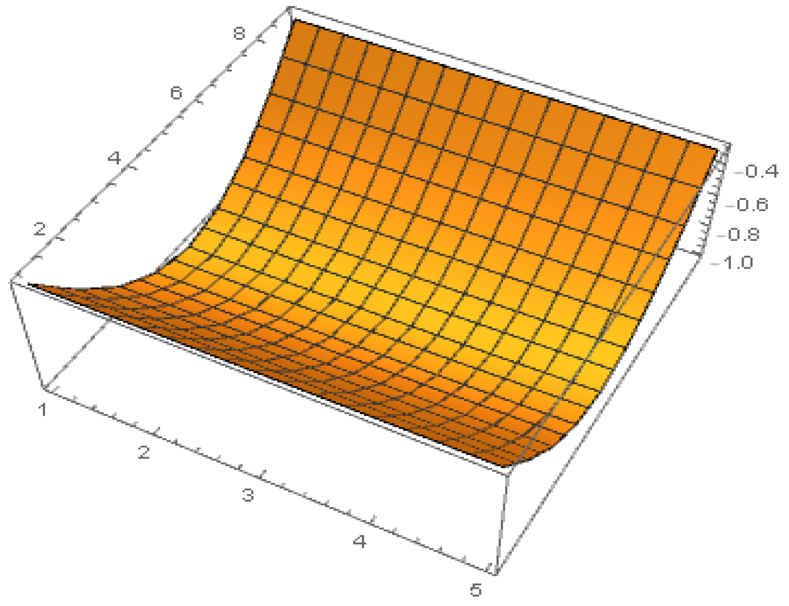
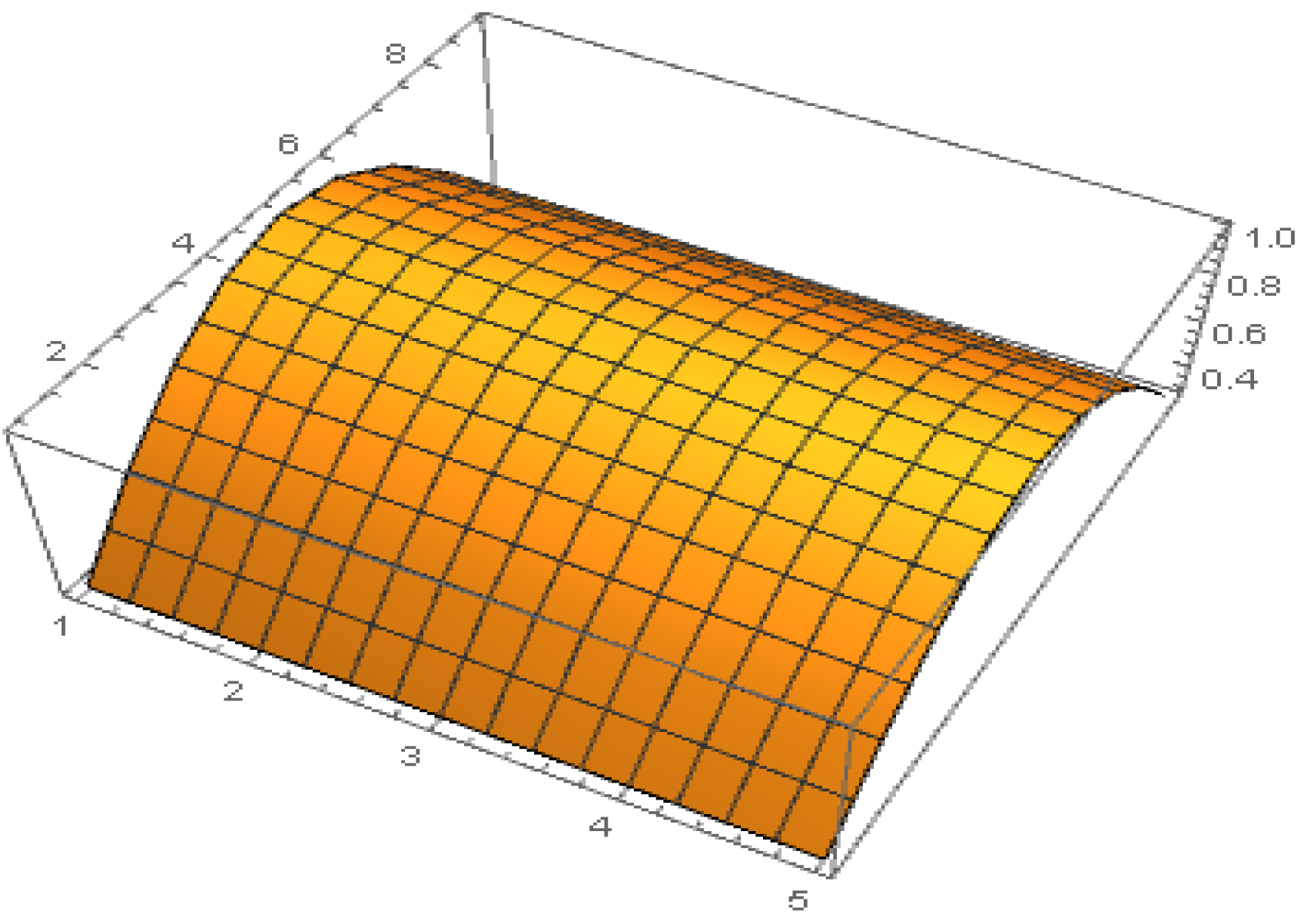
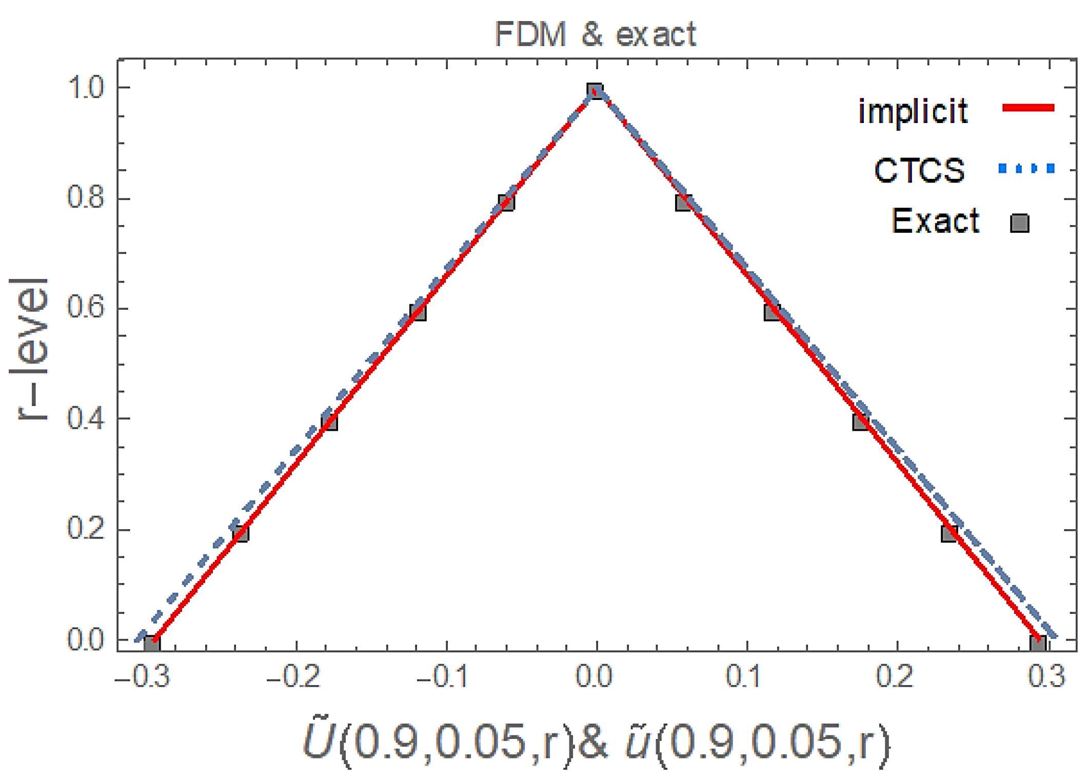
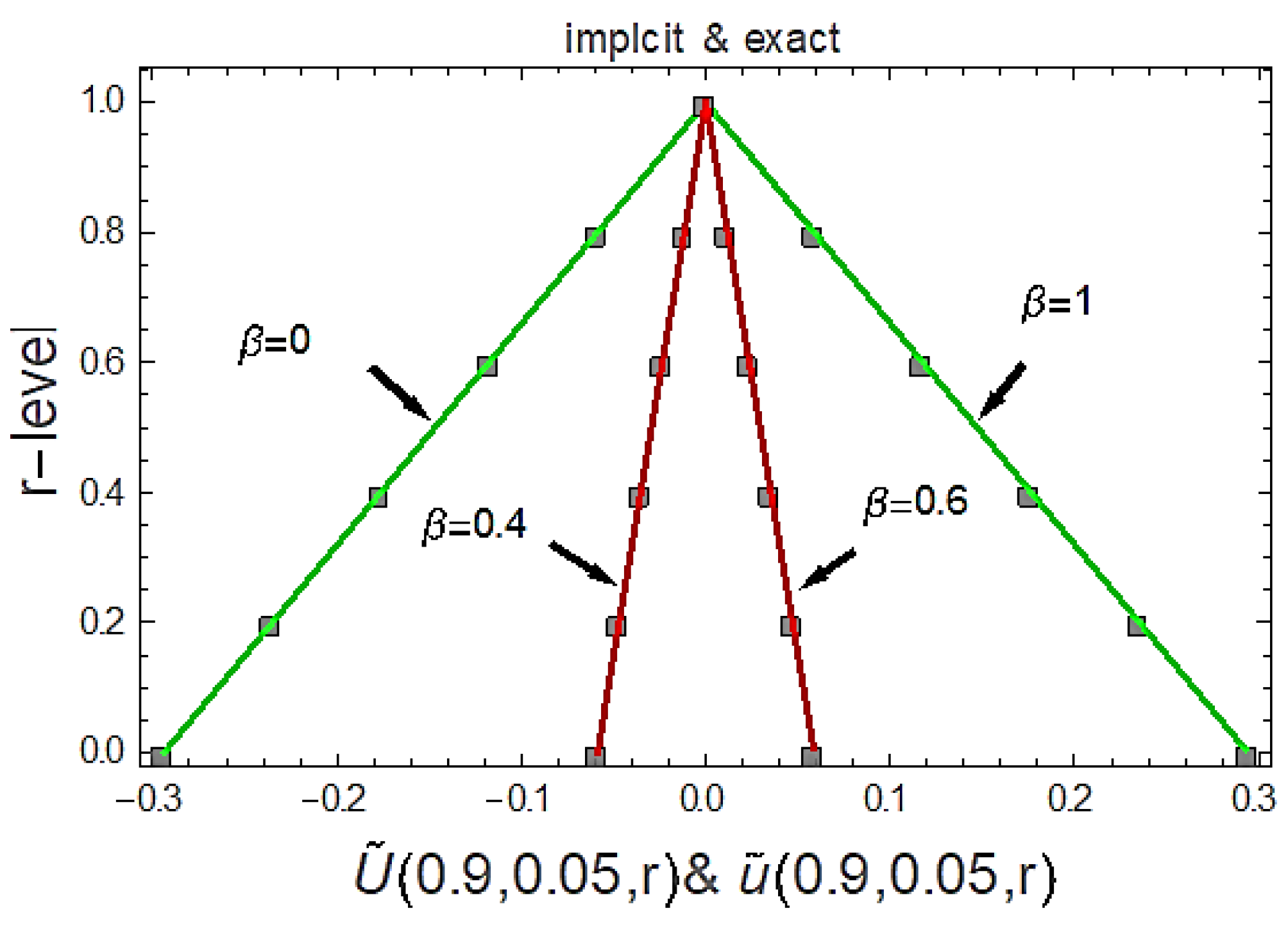
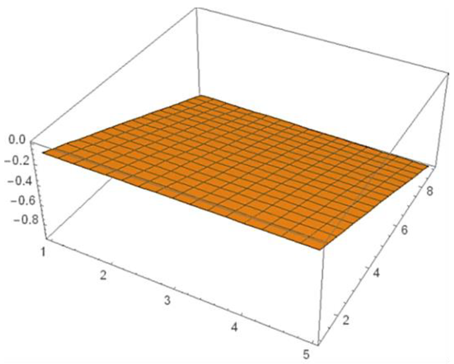
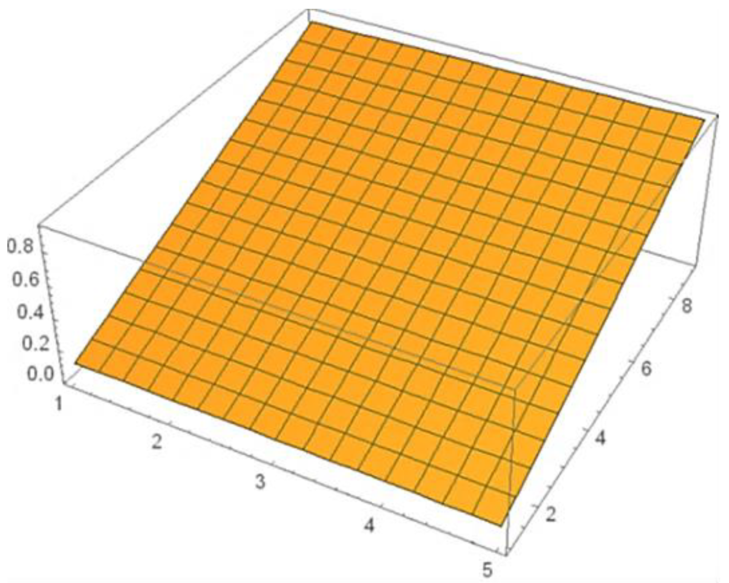
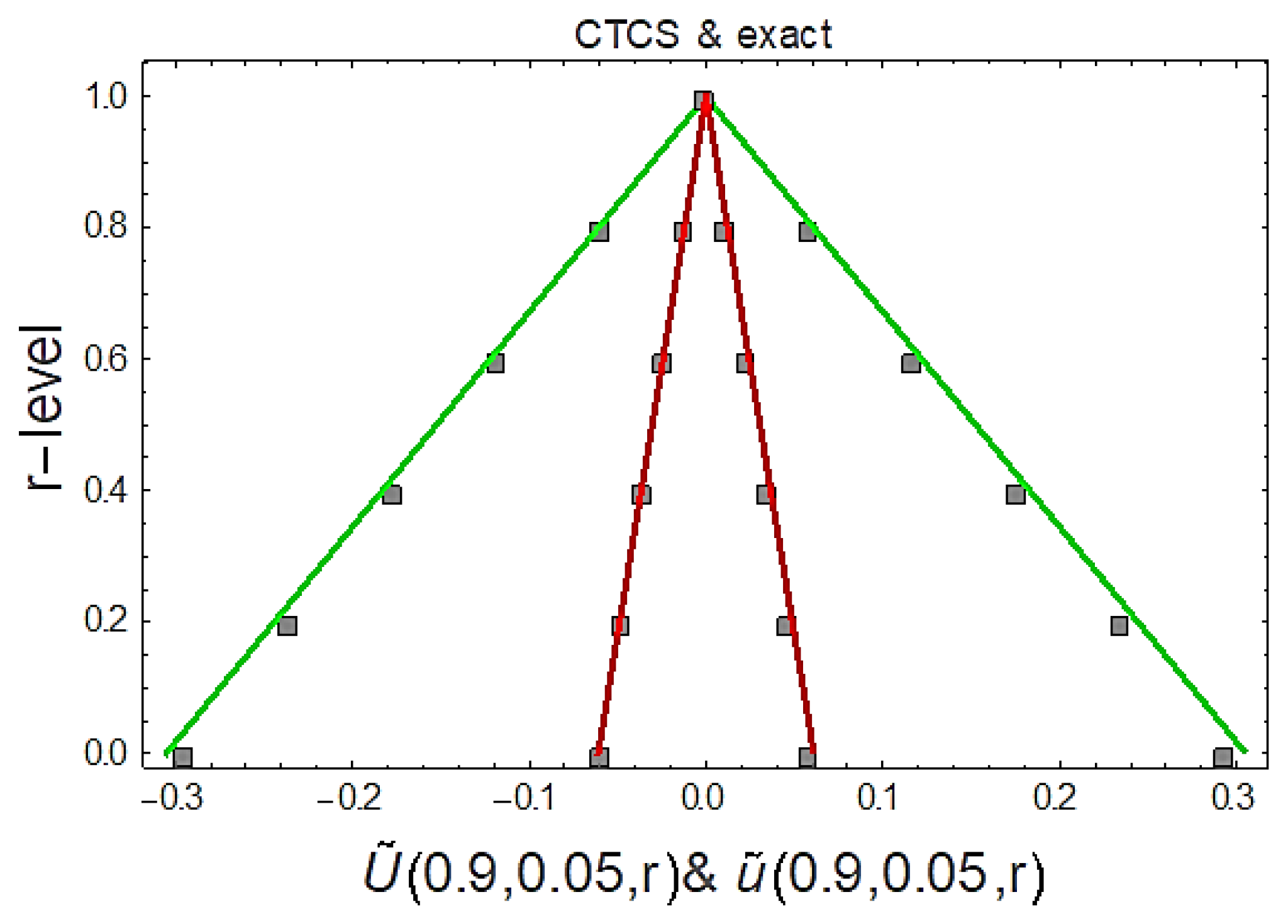
6. Numerical Examples and Solution Analysis

The implementation and review of Equation (1) numerical solutions through our proposed methods from Section 3 and Section 4 is discussed and compared in terms of accuracy with the exact solution, such that we defined the following two examples:

Example 6.1:

Consider the homogenous FWE [25]

$$\frac{{\partial }^2\tilde{u}\left(x,t\right)}{\partial t^2}=4 \frac{{\partial }^2\tilde{u}\left(x,t\right)}{\partial x^2},0<x<1, t>0.$$

(31)

where $\tilde{u}\left(0,t\right)=\tilde{u}\left(1,t\right)=0$ are boundary conditions and $\tilde{u}\left(x,0\right)=\tilde{\alpha } Sin\left(\pi x\right)$, $u_t\left(x,0\right)=0$ are the initial conditions of Equation (31) for

$$\tilde{\alpha }\left(r\right)=\left[r-1,1-r\right]$$

For $rϵ\left[0,1\right]$, it is clear that the partial derivative $\frac{{\partial }^2\tilde{u}\left(x,t\right)}{\partial t^2}$ and $\frac{{\partial }^2\tilde{u}\left(x,t\right)}{\partial x^2}$ follows the second case of generalized differentiability where the exact solution of Equation (31) is represented by the following equation and figures [25,29]:

$$\tilde{u}\left(x,t;r\right)=\tilde{\alpha }\left(r\right)Sin\left(\pi x\right)Cos\left(2\pi t\right).$$

(32)

According to double parametric form of the fuzzy number, the exact solution of Equation (31)$\mathrm{for} \mathrm{all} r,\beta \in \left[0,1\right]$ is as follows:

$$\tilde{u}\left(x,t;r;\beta \right)=\left(\left(\beta \left(2-2r\right)\right)+r-1\right)Sin\left(\pi x\right)Cos\left(2\pi t\right)$$

The numerical results in double parametric form that are obtained by CTCS at $∆x=h=0.1 \mathrm{and} ∆t=k=0.01 \mathrm{to} \mathrm{get} p=\frac{∆t^2}{∆x^2}=\frac{{0.01}^2}{{0.1}^2}$ are presented in the next tables and figure for different values of $r$ and $\beta$.

Table 1. Numerical solution of Equation (31) by CTCS and implicit at $t=0.05$ and $x=0.9$ for $r,\beta \in \left[0,1\right]$.

		CTCS		Implicit
$\beta$	$r$	$\tilde{u}\left(0.9,0.5;r,\beta \right)$	$\tilde{E}\left(0.9,0.5;r,\beta \right)$	$\tilde{u}\left(0.9,0.5;r,\beta \right)$	$\tilde{E}\left(0.9,0.5;r,\beta \right)$
Lower $\beta =0$	$0$	$-0.30897918419461035$	$1.14671\times {10}^{-4}$	$-0.3088657654966003$	$1.25235\times {10}^{-6}$
	$0.2$	$-0.247183347355688$	$9.17368\times {10}^{-5}$	$-0.24709261239728061$	$1.00188\times {10}^{-6}$
	$0.4$	$-0.1853875105167659$	$6.88026\times {10}^{-5}$	$-0.1853194592979603$	$7.51413\times {10}^{-7}$
	$0.6$	$-0.123591673677844$	$458684\times {10}^{-5}$	$-0.12354630619864031$	$5.00942\times {10}^{-7}$
	$0.8$	$-0.06179583683892198$	$2.29342\times {10}^{-5}$	$-0.06177315309932013$	$2.50471\times {10}^{-7}$
	$1$	0	0	0	0
Upper $\beta =1$	0	$0.30897918419461035$	$1.14671\times {10}^{-4}$	$0.3088657654966003$	$1.25235\times {10}^{-6}$
	0.2	$0.247183347355688$	$9.17368\times {10}^{-5}$	$0.24709261239728061$	$1.00188\times {10}^{-6}$
	0.4	$0.1853875105167659$	$6.88026\times {10}^{-5}$	$0.1853194592979603$	$7.51413\times {10}^{-7}$
	0.6	$0.123591673677844$	$458684\times {10}^{-5}$	$0.12354630619864031$	$5.00942\times {10}^{-7}$
	0.8	$0.06179583683892198$	$2.29342\times {10}^{-5}$	$0.06177315309932013$	$2.50471\times {10}^{-7}$
	1	0	0	0	0

and

Table 2. Numerical solution of Equation (31) by CTCS and implicit at $t=0.05$ and $x=0.9$ for $r,\beta \in \left[0,1\right].$

		CTCS		Implicit
$\beta$	$r$	$\tilde{u}\left(0.9,0.5;r,\beta \right)$	$\tilde{E}\left(0.9,0.5;r,\beta \right)$	$\tilde{u}\left(0.9,0.5;r,\beta \right)$	$\tilde{E}\left(0.9,0.5;r,\beta \right)$
$\beta =0$.4	$0$	$-0.06179583683892198$	$2.29342\times {10}^{-5}$	$-0.06177315309932013$	$2.50471\times {10}^{-7}$
	$0.2$	$-0.04943666947113756$	$1.83474\times {10}^{-5}$	$-0.0494185224794561$	$2.00377\times {10}^{-7}$
	$0.4$	$-0.0370775021033532$	$1.37605\times {10}^{-5}$	$-0.03706389185959205$	$1.50283\times {10}^{-7}$
	$0.6$	$-0.02471833473556878$	$9.17368\times {10}^{-6}$	$-0.02470926123972805$	$1.00188\times {10}^{-7}$
	$0.8$	$-0.012359167367784408$	$4.58684\times {10}^{-6}$	$-0.012354630619864042$	$5.00942\times {10}^{-8}$
	$1$	0	0	0	0
$\beta =0.6$	0	$0.06179583683892198$	$2.29342\times {10}^{-5}$	$0.06177315309932013$	$2.50471\times {10}^{-7}$
	0.2	$0.04943666947113756$	$1.83474\times {10}^{-5}$	$0.0494185224794561$	$2.00377\times {10}^{-7}$
	0.4	$0.0370775021033532$	$1.37605\times {10}^{-5}$	$0.03706389185959205$	$1.50283\times {10}^{-7}$
	0.6	$0.02471833473556878$	$9.17368\times {10}^{-6}$	$0.02470926123972805$	$1.00188\times {10}^{-7}$
	0.8	$0.012359167367784408$	$4.58684\times {10}^{-6}$	$0.012354630619864042$	$5.00942\times {10}^{-8}$
	1	0	0	0	0

, Figure 1 and Figure 2 clearly illustrate that both of the CTCS schemes have good results compared with the exact solution of Equation (31) at $t=0.05,x=0.9$ for all $r,\beta \in \left[0,1\right]$. In addition, the results obtained satisfy the characteristics of double parametric numbers by achieving a triangular fuzzy number shape and followed the second case of generalized differentiability. As shown in Figure 3, the implicit schemes tend to yield significantly more reliable results than CTCS. The transformation from uncertain to crisp has made it simple and effective to apply double parametric forms. In addition, it can be found that the results are more precise at points close to the inflection point $\beta =0.5,$ as shown in Figure 4.

Example 6.2:

Consider the FWE involving variable coefficient [30]:

$$\frac{{\partial }^2\tilde{u}\left(x,t\right)}{\partial t^2}=\frac{1}{2}{x}^2\frac{{\partial }^2\tilde{u}\left(x,t\right)}{\partial x^2}, 0<x<1, t>0$$

(33)

where the boundary conditions are $\tilde{u}\left(0,t\right)=t$, $\tilde{u}\left(1,t\right)=1+\sinh t$ and the initial fuzzy conditions $\tilde{u}\left(x,0\right)=\tilde{\alpha } x$,$u_t\left(x,0\right)=x^2$ of Equation (33) for $\tilde{\alpha }=\left[r-1,1-r\right]$.

For $rϵ\left[0,1\right]$, it is clear that the partial derivative $\frac{{\partial }^2\tilde{u}\left(x,t\right)}{\partial t^2}$ and $\frac{{\partial }^2\tilde{u}\left(x,t\right)}{\partial x^2}$ follows the first case of the generalized differentiability where the exact solution of Equation (33) was given in [30] (see Figure 5 and Figure 6) such that:

$$\tilde{u}\left(x,t;r\right)=\tilde{\alpha }\left(r\right)\left(x+x^2\sinh t\right)$$

(34)

The numerical results in double parametric form that are obtained by $∆x=h=0.1 \mathrm{and} ∆t=k=0.01 \mathrm{to} \mathrm{get} p=\frac{∆t^2}{∆x^2}=\frac{{0.01}^2}{{0.1}^2}$ are presented in the next tables and figure for different values of $r$ and $\beta$.

Similarly to example 6.1,

Table 3. Numerical solution of Equation (33) by CTCS and implicit at $t=0.05$ and $x=0.9$ for $r,\beta \in \left[0,1\right].$

		CTCS		Implicit
$\beta$	$r$	$\tilde{u}\left(0.9,0.5;r,\beta \right)$	$\tilde{E}\left(0.9,0.5;r,\beta \right)$	$\tilde{u}\left(0.9,0.5;r,\beta \right)$	$\tilde{E}\left(0.9,0.5;r,\beta \right)$
Lower $\beta =0$	$0$	$-0.30553524551329963$	$1.635507\times {10}^{-2}$	$-0.2940107401726$	$1.4547205\times {10}^{-4}$
	$0.2$	$-0.23535441946397$	$9.0580554\times {10}^{-3}$	$-0.2352085921381$	$1.157764\times {10}^{-4}$
	$0.4$	$-0.1833535114597978$	$6.85104\times {10}^{-3}$	$-0.1764064884410$	$8.853232\times {10}^{-5}$
	$0.6$	$-0.12513322097319855$	$4.544027\times {10}^{-3}$	$-0.117604296069$	$5.858821\times {10}^{-5}$
	$0.8$	$-0.0651351048659927$	$2.247013\times {10}^{-3}$	$-0.058802148034$	$2.954411\times {10}^{-5}$
	$1$	0	0	0	0
Upper $\beta =1$	0	$0.30513524329963$	$1.143507\times {10}^{-2}$	$0.2940107401726$	$1.457205\times {10}^{-4}$
	0.2	$0.2441946397$	$9.408054\times {10}^{-3}$	$0.2352085921381$	$1.175764\times {10}^{-4}$
	0.4	$0.183145597978$	$6.8163404\times {10}^{-3}$	$0.1764064884410$	$8.83232\times {10}^{-5}$
	0.6	$0.1220957319855$	$4.54027\times {10}^{-3}$	$0.117604296069$	$5.88821\times {10}^{-5}$
	0.8	$0.0610548659927$	$2.2705413\times {10}^{-3}$	$0.058802148034$	$2.94411\times {10}^{-5}$
	1	0	0	$0$	0

and

Table 4. Numerical solution of Equation (33) by CTCS and implicit at $t=0.05$ and $x=0.9$ for $r,\beta \in \left[0,1\right]$.

		CTCS		Implicit
$\beta$	$r$	$\tilde{u}\left(0.9,0.5;r,\beta \right)$	$\tilde{E}\left(0.9,0.5;r,\beta \right)$	$\tilde{u}\left(0.9,0.5;r,\beta \right)$	$\tilde{E}\left(0.9,0.5;r,\beta \right)$
$\beta =0$.4	$0$	$-0.06145361048659927$	$2.270113\times {10}^{-3}$	$-0.05880796628017$	$2.94411\times {10}^{-5}$
	$0.2$	$-0.04156651458838927942$	$1.8154611\times {10}^{-3}$	$-0.04704637302416$	$2.35528\times {10}^{-5}$
	$0.4$	$-0.0513536629195956$	$1.34656208\times {10}^{-3}$	$-0.0354545628477976810$	$1.76646\times {10}^{-5}$
	$0.6$	$-0.0251564419463971$	$9.0458054\times {10}^{-4}$	$-0.02354654552318651207$	$1.17764\times {10}^{-5}$
	$0.8$	$-0.01531532209731985$	$4.54027\times {10}^{-4}$	$-0.01176159325603$	$5.88821\times {10}^{-6}$
	$1$	0	0	0	0
$\beta =0.6$	0	$0.061051548659927$	$2.27013\times {10}^{-3}$	$0.05880796628017$	$2.94411\times {10}^{-5}$
	0.2	$0.048838927942$	$1.81611\times {10}^{-3}$	$0.04704637302416$	$2.35528\times {10}^{-5}$
	0.4	$0.0365445629195956$	$1.3654208\times {10}^{-3}$	$0.0355428477976810$	$1.764646\times {10}^{-5}$
	0.6	$0.02441549415463971$	$9.0854054\times {10}^{-4}$	$0.02345652318651207$	$1.14567764\times {10}^{-5}$
	0.8	$0.012204559731985$	$4.544027\times {10}^{-4}$	$0.01154576159325603$	$5.8468821\times {10}^{-6}$
	1	0	0	0	0

, Figure 5 and Figure 6 clearly illustrate the of both the CTCS schemes have good results compared with the exact solution of Equation (27) at $t=0.05,x=0.9$ for all $r,\beta \in \left[0,1\right]$. In addition, the results obtained satisfy the characteristics of double parametric numbers by achieving a triangular fuzzy number shape and followed the first case of generalized differentiability. Implicit schemes tend to yield significantly more reliable results than CTCS. The transformation from uncertain to crisp has made it simple and effective to apply double parametric forms. In addition, it can be found that the results are more precise at points close to the inflection point $\beta =0.5$ as shown in Figure 7.

7. Summary

In this paper, a new extension of finite difference schemes was suggested to solve general FWEs in terms of the double parametric form of fuzzy number. The schemes incorporating the double parametric form of fuzzy number were formulated and analyzed to obtain the numerical solution for the FWE. The implicit scheme tends to yield significantly more accurate results than the CTCS scheme. Stability analysis is illustrated followed by the proof of stability theorem for CTCS under the double parametric form of fuzzy numbers and has accuracy in the order of $O\left(∆t^2+∆x^2\right)$. The results obtained from two numerical examples indicated good agreement with the exact solution and follow the properties of triangular fuzzy numbers. The proposed method can be extended for neutrosophic statistics [31,32] as future research and this will be investigated in detail at a later stage.

References

1. Amoddeo, A. Moving mesh partial differential equations modelling to describe oxygen induced effects on avascular tumour growth. Cogent Phys. 2015, 2, 1050080. [Google Scholar] [CrossRef]
2. Holmes, E.E.; Lewis, M.A.; Banks, J.E.; Veit, R.R. Partial Differential Equations in Ecology: Spatial Interactions and Population Dynamics. Ecology 1994, 75, 17–29. [Google Scholar] [CrossRef]
3. Stockar, S.; Canova, M.; Guezennec, Y.; Rizzoni, G. A Lumped-Parameter Modeling Methodology for One-Dimensional Hyperbolic Partial Differential Equations Describing Nonlinear Wave Propagation in Fluids. J. Dyn. Syst. Meas. Control. 2014, 137, 011002. [Google Scholar] [CrossRef]
4. Macías-Díaz, J.; Tomasiello, S. A differential quadrature-based approach à la Picard for systems of partial differential equations associated with fuzzy differential equations. J. Comput. Appl. Math. 2016, 299, 15–23. [Google Scholar] [CrossRef]
5. Sarmad, A.A.; Ali, F.J.; Azizan, S. A Single Convergent Control Parameter Optimal Homotopy Asymptotic Method Approximate-Analytical Solution of Fuzzy Heat Equation. ASM Sci. J. 2019, 12, 42–47. [Google Scholar]
6. Nemati, K.; Matinfar, M. An implicit method for fuzzy parabolic partial differential equations. J. Nonlinear Sci. Appl. 2008, 1, 61–71. [Google Scholar] [CrossRef] [Green Version]
7. Allahviranloo, T.; Kermani, A.M. Numerical Methods for Fuzzy Partial Differential Equations under New Defini-tion For Derivative. Iran. J. Fuzzy Syst. 2010, 7, 33–50. [Google Scholar]
8. Zureigat, H.H.; Ismail, A.I.M. Numerical solution of fuzzy heat equation with two different fuzzifications. In Proceedings of the 2016 SAI Computing Conference (SAI), London, UK, 13–15 July 2016; pp. 85–90. [Google Scholar]
9. Abdi, M.; Allahviranloo, T. Fuzzy finite difference method for solving fuzzy Poisson’s equation. J. Intell. Fuzzy Syst. 2019, 37, 5281–5296. [Google Scholar] [CrossRef]
10. Aminzadeh, F. Applications of AI and soft computing for challenging problems in the oil industry. J. Pet. Sci. Eng. 2005, 47, 5–14. [Google Scholar] [CrossRef]
11. He, J.-H. Some asymptotic methods for strongly nonlinear equations. Int. J. Mod. Phys. B 2006, 20, 1141–1199. [Google Scholar] [CrossRef] [Green Version]
12. Wang, F.Y.; Liu, D. Networked Control Systems. In Theory and Applications; Springer: Berlin/Heidelberg, Germany, 2008. [Google Scholar]
13. Zheng, Y.-J. Water wave optimization: A new nature-inspired metaheuristic. Comput. Oper. Res. 2015, 55, 1–11. [Google Scholar] [CrossRef] [Green Version]
14. Long, H.V.; Nieto, J.J.; Son, N.T.K. New approach for studying nonlocal problems related to differential systems and partial differential equations in generalized fuzzy metric spaces. Fuzzy Sets Syst. 2018, 331, 26–46. [Google Scholar] [CrossRef]
15. Allahviranloo, T.; Abbasbandy, S.; Rouhparvar, H. The exact solutions of fuzzy wave-like equations with variable coefficients by a variational iteration method. Appl. Soft Comput. 2011, 11, 2186–2192. [Google Scholar] [CrossRef]
16. Chadli, L.S.; Harir, A.; Melliani, S. Solutions of fuzzy wave-like equations by variational iteration method. Int. Ann. Fuzzy Math. Inform. 2014, 8, 527–547. [Google Scholar]
17. Hashemi, M.; Malekinagad, J. Series solution of fuzzy wave-like equations with variable coefficients. J. Intell. Fuzzy Syst. 2013, 25, 415–428. [Google Scholar] [CrossRef]
18. Bayrak, M.A. Approximate Solution of Wave Equation using Fuzzy Number. Int. J. Comput. Appl. 2013, 68, 975. [Google Scholar]
19. Zureigat, H.; Ismail, A.I.; Sathasivam, S. A compact Crank–Nicholson scheme for the numerical solution of fuzzy time fractional diffusion equations. Neural Comput. Appl. 2019, 32, 6405–6412. [Google Scholar] [CrossRef]
20. Cheng, C. Fuzzy Solutions to Partial Differential Equations: Adaptive Approach. IEEE Trans. Fuzzy Syst. 2009, 17, 116–127. [Google Scholar] [CrossRef]
21. Bodjanova, S. Median alpha-levels of a fuzzy number. Fuzzy Sets Syst. 2006, 157, 879–891. [Google Scholar] [CrossRef]
22. George, J.; Bo, Y. Fuzzy Sets and Fuzzy Logic, Theory and Applications; Prentice Hall Publishing: Upper Saddle River, NJ, USA, 1995. [Google Scholar]
23. Zadeh, L.A. Fuzzy sets as a basis for a theory of possibility. Fuzzy Sets Syst. 1978, 1, 3–28. [Google Scholar] [CrossRef]
24. Zadeh, L.A. Toward a generalized theory of uncertainty (GTU)—An outline. Inf. Sci. 2005, 172, 1–40. [Google Scholar] [CrossRef]
25. Kermani, M.A. Numerical method for solving fuzzy wave equation. AIP Conf. Proc. 2013, 1558, 2444–2447. [Google Scholar] [CrossRef]
26. Allahviranloo, T.; Gouyandeh, Z.; Armand, A.; Hasanoglu, A. On fuzzy solutions for heat equation based on gen-eralized Hukuhara differentiability. Fuzzy Sets Syst. 2015, 265, 1–23. [Google Scholar] [CrossRef]
27. Chakraverty, S.; Tapaswini, S.; Behera, D. Fuzzy Differential Equations and Applications for Engineers and Scientists; CRC Press: Boca Raton, FL, USA, 2016. [Google Scholar]
28. Oishi, C.M.; Yuan, J.Y.; Cuminato, J.A.; Stewart, D.E. Stability analysis of Crank–Nicolson and Euler schemes for time-dependent diffusion equations. BIT Numer. Math. 2015, 55, 487–513. [Google Scholar] [CrossRef]
29. Allahviranloo, T. Difference Methods for Fuzzy Partial Differential Equations. Comput. Methods Appl. Math. 2002, 2, 233–242. [Google Scholar] [CrossRef]
30. Alhayani, W. Exact solutions for heat-like and wave-like equations with variable coefficients by daftardar-jafari method. Far East J. Appl. Math. 2014, 87, 191. [Google Scholar]
31. Smarandache, F. Neutrosophic logic-a generalization of the intuitionistic fuzzy logic. Multispace Multistruct. 2010, 4, 396. [Google Scholar] [CrossRef] [Green Version]
32. Aslam, M. Neutrosophic analysis of variance: Application to university students. Complex Intell. Syst. 2019, 5, 403–407. [Google Scholar] [CrossRef] [Green Version]
Figure 1. The lower exact solution of Equation (31) at t = 0.01 , x = 0.1 , r = 0   and   β = 1 .
Mathematics 09 00667 g001
Figure 2. The upper exact solution of Equation (31) at t = 0.01 , x = 0.1 ,   r = 0   and   β = 1 .
Mathematics 09 00667 g002
Figure 3. The exact and numerical solution of Equation (31) by CTCS and implicit schemes at t = 0.05 and x = 0.9 for all r , β [ 0 , 1 ] .
Mathematics 09 00667 g003
Figure 4. The exact and numerical solution of Equation (31) by implicit at t = 0.5 and x = 0.9 for all r , β [ 0 , 1 ] .
Mathematics 09 00667 g004
Figure 5. The exact solution (lower solution) of Equation (33) at t = 0.01 , x 0.1 , r = 0   and   β = 0 .
Mathematics 09 00667 g005
Figure 6. The exact solution (upper solution) of Equation (33) at   t = 0.01 , x 0.1 , r = 0   and   β = 0 .
Mathematics 09 00667 g006
Figure 7. The exact and numerical solution of Equation (33) implicit at t = 0.05 and x = 0.9 for all r , β [ 0 , 1 ] .
Mathematics 09 00667 g007