Recognition and Analysis of Image Patterns Based on Latin Squares by Means of Computational Algebraic Geometry

Abstract

With the particular interest of being implemented in cryptography, the recognition and analysis of image patterns based on Latin squares has recently arisen as an efficient new approach for classifying partial Latin squares into isomorphism classes. This paper shows how the use of a Computer Algebra System (CAS) becomes necessary to delve into this aspect. Thus, the recognition and analysis of image patterns based on these combinatorial structures benefits from the use of computational algebraic geometry to determine whether two given partial Latin squares describe the same affine algebraic set. This paper delves into this topic by focusing on the use of a CAS to characterize when two partial Latin squares are either partial transpose or partial isotopic.

1. Introduction

An $n\times n$ array is said to be a partial Latin square of order n if each one of its cells either is empty or contains an element of a finite set of n symbols so that each symbol occurs at most once in each row and at most once in each column. If there are no empty cells, then the array is called a Latin square. Latin squares play a relevant role in cryptography [1,2,3]. Of particular interest for the aim of this paper, the generation of scramblers in symmetric cryptography by means of encryption–decryption processes having Latin squares as cryptographic keys is remarkable [4,5,6,7,8]. The exponential growth of Latin squares [9,10,11] ensures the robustness of these symmetric-key algorithms against brute force and statistical attacks. In addition, appropriate choices of Latin squares produce effective symmetric-key algorithms with high period growths [12]. In this regard, the distribution of Latin squares into isomorphism classes play a fundamental role. It is so that pseudo-random sequences derived from non-isomorphic Latin squares give rise to certain image patterns [13,14], whose algebraic and geometrical properties enable one to distinguish between fractal and non-fractal Latin squares [15,16].

Distributing (partial) Latin squares into isomorphism classes indeed constitutes a main problem in the theory of (partial) Latin squares. Currently, only the number of isomorphism classes of Latin squares of order $n\le 11$ is known [9,10,11], as well as that of partial Latin squares of order $n\le 6$ [17,18]. To obtain these last values, the computation of reduced Gröbner bases of ideals associated to partial Latin squares has played a relevant role. Such a computation is, however, extremely sensitive to the number of involved variables and the length and degree of the corresponding generators [19,20,21,22]. Thus, although distinct techniques concerning computational algebraic geometry have been implemented since the original work of Bayer [23] for solving the classical problems of counting, enumerating and classifying partial Latin squares [17,18,24,25,26,27,28,29] and solving related problems such as completing sudokus [30,31,32], their computational cost makes it very difficult to deal with partial Latin squares of high orders.

The study of new invariants concerning partial Latin square isomorphisms has turned out to be an optimal approach to reduce this computational cost [33,34,35]. This paper delves in particular into those invariants that are related to affine algebraic sets associated to the partial Latin squares under consideration. In this regard, let us recall that the affine algebraic set in a multivariate polynomial ring $\mathbb{K}\left[\{x_1,\dots ,x_n\}\right]$ of a partial Latin square $L=\left(l_{i,j}\right)$ of order n, with set of symbols $\left[n\right]:=\{1,\dots ,n\}$, was defined by Falcón, R.M. et al [36] as the set of zeros of the binomial ideal

$$I\left(L\right):=〈x_i{x}_j-x_{l_{i,j}}:1\le i,j,l_{i,j}\le n〉.$$

(1)

Isomorphic partial Latin squares give rise to isomorphic affine algebraic sets. Thus, Gröbner bases have played a relevant role for distinguishing, in a computationally fast way, image patterns arisen from non-isomorphic Latin squares. In any case, the study of affine algebraic sets associated to Latin squares is still in the very initial stage. Thus, for instance, their distribution into isomorphism classes is only known for $n\le 3$ [36]. To deal with higher orders, it is necessary to delve into two new ways of classifying partial Latin squares. More specifically, it is necessary to characterize when two partial Latin squares are partial transpose and/or partial isotopic. In both cases, the partial Latin squares under consideration may give rise to the same affine algebraic set.

The paper is organized as follows. Section 2 deals with some preliminary concepts and results on partial Latin squares and computational algebraic geometry that are used throughout the paper. In Section 3, the notion of standard set of image patterns associated to a Latin square is introduced, which may constitute a fast computational way for distinguishing non-isomorphic Latin squares. To this end, the use of a new affine algebraic set associated to each of these image patterns is proposed. Finally, two new ideals are described in Section 4, whose respective affine algebraic sets are uniquely identified with the set of partial Latin squares that are partial transpose of another given partial Latin square, and the set of partial isotopisms between two given partial Latin squares of the same order and weight.

2. Preliminaries

Let us review some basic concepts and results on partial Latin squares and computational algebraic geometry that are used throughout the paper. We refer the reader to the monographs of [37,38] for more details on both topics.

2.1. Partial Latin Squares

Let ${\mathcal{L}}_n$ be the set of partial Latin squares of order n having the already mentioned set $\left[n\right]$ as set of symbols. Every partial Latin square $L=\left(l_{i,j}\right)\in {\mathcal{L}}_n$ is determined by its set of entries

$$\mathrm{Ent}\left(L\right):=\{(i,j,l_{i,j}):i,j,l_{i,j}\in \left[n\right]\}.$$

Therefore, the cardinality of this set coincides with the number of non-empty cells within the partial Latin square L. It is termed the weight of L. From here on, let ${\mathcal{L}}_{n;m}$ denote the subset of partial Latin squares in the set ${\mathcal{L}}_n$ of weight m.

Let $S_n$ denote the symmetric group on the set $\left[n\right]$. Every triple $\theta =(f,g,h)\in S_n^3$ preserves the set ${\mathcal{L}}_{n;m}$. It constitutes an isotopism of partial Latin squares, where the bijections f, g and h correspond, respectively, to a permutation of rows, a permutation of columns and a permutation of symbols of the partial Latin square under consideration. More specifically, the isotopism $\theta$ acts on any given partial Latin square $L\in {\mathcal{L}}_{n;m}$ by giving rise to its isotopic partial Latin square $L^{\theta }\in {\mathcal{L}}_{n;m}$, where

$$\mathrm{Ent}\left(L^{\theta }\right)=\{(f\left(i\right),g\left(j\right),h\left(k\right)):(i,j,k)\in \mathrm{Ent}\left(L\right)\}.$$

If $f=g=h$, then the isotopism $\theta$ constitutes an isomorphism. In such a case, the partial Latin squares L and $L^{\theta }$ are said to be isomorphic. Throughout this paper, the computation of isotopisms and isomorphisms among partial Latin squares is done by making respective use of the procedures isot and isom of the library pls.lib, available online at http://personales.us.es/raufalgan/LS/pls.lib (accessed on 28 February 2021), for the open Computer Algebra System (CAS) for polynomial computations SINGULAR [39].

Isotopic and isomorphic are equivalence relations among partial Latin squares. The distribution into such classes is known for order $n\le 11$ in the case of dealing with Latin squares [9,10,11] and for order $n\le 6$ in the case of dealing with partial Latin squares [17,18]. Partial transpose are partial isotopic are two other binary relations among partial Latin squares of the same order and weight, whose study is still in teh very initial stage. Although the original definitions were established by Falcón, R.M. et al [36] as equivalence relations, it is not so. In what follows, we particularize both definitions in order to obtain two new equivalence relations among partial Latin squares of the same order and weight. To this end, let us consider two partial Latin squares $L_1$ and $L_2$ in ${\mathcal{L}}_{n;m}$.

We say that $L_2$ is partial transpose of $L_1$ if and only if the following two conditions hold.

• For each entry $(i,j,k)\in \mathrm{Ent}\left(L_2\right)\backslash \mathrm{Ent}\left(L_1\right)$, we have that $(j,i,k)\in \mathrm{Ent}\left(L_1\right)$.
• For each entry $(i,j,k)\in \mathrm{Ent}\left(L_1\right)\backslash \mathrm{Ent}\left(L_2\right)$, we have that $(j,i,k)\in \mathrm{Ent}\left(L_2\right)$.

Being partial transpose generalizes, therefore, the classical concept of being transpose. Notice that the second condition that we have just described was not explicitly indicated by Falcón, R.M. et al [36]. Nevertheless, as is illustrated in the following example, this condition is mandatory in order to obtain a symmetric relation.

Example 1.

The partial Latin squares

$$L_1\equiv \boxed{\begin{array}{cccc}1& 2& 3& \\ & & 4& 3\\ 4& & 1& \\ & & 2& \end{array}}and{L}_2\equiv \boxed{\begin{array}{cccc}1& 2& 4& \phantom{4}\\ 2& & & \\ 3& 4& 1& \\ & & 2& \end{array}},$$

both of them in ${\mathcal{L}}_{4;8}$, satisfy the first described condition in order to ensure that $L_2$ is partial transpose of $L_1$. Nevertheless, such a condition is not satisfied for ensuring that $L_1$ is partial transpose of $L_2$, because the entry $(2,4,3)\in \mathrm{Ent}\left(L_1\right)\backslash \mathrm{Ent}\left(L_2\right)$ and $(4,2,3)\notin \mathrm{Ent}\left(L_2\right)$.

Now, let $P\subseteq \mathrm{Ent}\left(L_1\right)\cap \mathrm{Ent}\left(L_2\right)$. We say that $L_2$ is P-partial isotopic to $L_1$ if there exists an isotopism $(f,g,h)\in S_n^3$ such that

$$\mathrm{Ent}\left(L_2\right)\backslash P=\{(f\left(i\right),g\left(j\right),h\left(k\right)):(i,j,k)\in \mathrm{Ent}\left(L_1\right)\backslash P\}.$$

In such a case, we say that the triple $(f,g,h)$ is a P-partial isotopism (a partial isotopism, when there is no place for confusion) from $L_1$ to $L_2$. The just described binary relation of being P-partial isotopic constitutes an equivalence relation among partial Latin squares of the same order and weight, as well as containing the subset P in their respective sets of entries. Further, if two partial Latin squares are isotopic, then they are ∅-partial isotopic. More specifically, every isotopism from $L_1$ to $L_2$ is also a partial isotopism between such partial Latin squares.

The subset $P\subseteq \mathrm{Ent}\left(L_1\right)\cap \mathrm{Ent}\left(L_2\right)$ was not established as an essential part of the original definition of being partial isotopic introduced by Falcón, R.M. et al. [36]. Nevertheless, if it is not considered as such, then the resulting binary relation is intransitive. The following example illustrates this fact. In this example, and from now on, to make much clearer the understanding of the subset P associated to any given partial isotopism in $S_n^3$, we denote $L\left(P\right)$ the partial Latin square of order n satisfying that $\mathrm{Ent}\left(L\right(P\left)\right)=P$.

Example 2.

The Latin squares

$$L_1\equiv \boxed{\begin{array}{cccc}1& 2& 3& 4\\ 2& 1& 4& 3\\ 4& 3& 2& 1\\ 3& 4& 1& 2\end{array}}and{L}_2\equiv \boxed{\begin{array}{cccc}1& 2& 3& 4\\ 2& 1& 4& 3\\ 3& 4& 1& 2\\ 4& 3& 2& 1\end{array}}$$

are isotopic (and, hence, ∅-partial isotopic) by means of the isotopism $(\left(34\right),\mathrm{Id},\mathrm{Id})\in S_4^3$, that is, by switching their third and fourth rows. It is readily verified that the Latin square $L_2$ is P-partial isotopic to

$$L_3\equiv \boxed{\begin{array}{cccc}1& 2& 3& 4\\ 2& 4& 1& 3\\ 3& 1& 4& 2\\ 4& 3& 2& 1\end{array}}$$

where $P=\mathrm{Ent}\left(L_2\right)\cap \mathrm{Ent}\left(L_3\right)$. That is,

$$L\left(P\right)\equiv \boxed{\begin{array}{cccc}1& 2& 3& 4\\ 2& & & 3\\ 3& & & 2\\ 4& 3& 2& 1\end{array}}$$

To this end, it is enough to consider, for instance, the partial isotopism $(\left(23\right),\mathrm{Id},\mathrm{Id})\in S_4^3$. Nevertheless, as shown in Example 8, no partial isotopism exists from $L_1$ to $L_3$.

The following example illustrates all the previous definitions in case of dealing with partial Latin squares with empty cells.

Example 3.

The partial Latin squares

$$L_1\equiv \boxed{\begin{array}{cccc}1& 2& 3& \\ & & 4& 3\\ 4& & 1& \\ & & 2& \end{array}}\mathrm{and}{L}_2\equiv \boxed{\begin{array}{cccc}1& 2& 4& \phantom{4}\\ & & & \\ 3& 4& 1& \\ & 3& 2& \end{array}},$$

both of them in the set ${\mathcal{L}}_{4;8}$, are partial transpose of each other. Notice, for instance, that the first condition of the definition holds because

$$\mathrm{Ent}\left(L_2\right)\backslash \mathrm{Ent}\left(L_1\right)=\{(1,3,4),(3,1,3),(3,2,4),(4,2,3)\}$$

and

$$\{(3,1,4),(1,3,3),(2,3,4),(2,4,3)\}\subset \mathrm{Ent}\left(L_1\right).$$

The second condition holds similarly. In addition, one can find a partial isotopism between both partial Latin squares $L_1$ and $L_2$. To this end, it is enough to consider the isotopism $\theta =(\left(1423\right),\left(1324\right),\mathrm{Id})\in S^3$ and the subset $P=\mathrm{Ent}\left(L_1\right)\cap \mathrm{Ent}\left(L_2\right)$. That is,

$$L\left(P\right)\equiv \boxed{\begin{array}{cccc}1& 2& & \phantom{4}\\ & & & \\ & & 1& \\ & & 2& \end{array}}\in {\mathcal{L}}_{4;4}$$

In particular,

$$L{\left(\mathrm{Ent}\left(L_1\right)\backslash P\right)}^{\theta }=L\left(\mathrm{Ent}\left(L_2\right)\backslash P\right)\equiv \boxed{\begin{array}{cccc}& & 4& \phantom{4}\\ & & & \\ 3& 4& & \\ & 3& & \end{array}}\in {\mathcal{L}}_{4;4}.$$

Notice that both partial Latin squares $L_1$ and $L_2$ are neither transpose nor isotopic of each other.

Let us finish this subsection by focusing on the description of the image patterns based on a given Latin square. To this end, let us recall that every Latin square in the set ${\mathcal{L}}_{n;n^2}$ constitutes the multiplication table of a quasigroup $\left(\right[n],·)$, where the set $\left[n\right]$ is endowed with a binary operation · so that the equations $a·x=b$ and $y·a=b$ have unique solutions for x and y in $\left[n\right]$, for all $a,b\in \left[n\right]$. Equivalently, the set $\left[n\right]$ is endowed with a left-division \ and a right-division /, so that $x=a\backslash b$ in the first equation, and $y=b/a$ in the second one.

Let $T=t_1{t}_2\dots t_m$ be a plaintext, with $t_i\in \left[n\right]$, for all $i\le m$. For each positive integer $s\le n$, it is defined [6,7,8] the encrypted string

$$E_s\left(T\right):=e_1{e}_2\dots e_m,$$

where

$$e_i:=\left\{\begin{array}{c}\begin{array}{cc}s·t_1,\hfill & \mathrm{if}i=1,\hfill \\ e_{i-1}·t_i,\hfill & \mathrm{otherwise}.\hfill \end{array}\hfill \end{array}\right.$$

The resulting string can be desencrypted by means of a decryption map $D_s$ based on the already mentioned left-division. More specifically,

$$t_i=\left\{\begin{array}{c}\begin{array}{cc}s\backslash e_1,\hfill & \mathrm{if}i=1,\hfill \\ e_{i-1}\backslash e_i,\hfill & \mathrm{otherwise}.\hfill \end{array}\hfill \end{array}\right.$$

The sequential implementation of the just described encryption may give rise to image patterns with certain fractal properties [13,14,15,16]. More specifically, if $S=(s_1,\dots ,s_{r-1})$ is an $(r-1)$-tuple of positive integers such that $s_i\le n$, for all $i<r$, then the $r\times m$ image pattern ${\mathcal{P}}_{S,T}\left(L\right)=\left(p_{i,j}\right)$ is defined as the $r\times m$ array satisfying that, for each positive integer $j\le m$, we have that

$$p_{i,j}:=\left\{\begin{array}{c}\begin{array}{cc}{t}_j,\hfill & \mathrm{if}i=1,\hfill \\ s_{i-1}·p_{i-1,1},\hfill & \mathrm{if}i>1\mathrm{and}j=1,\hfill \\ p_{i,j-1}·p_{i-1,j},\hfill & \mathrm{otherwise}.\hfill \end{array}\hfill \end{array}\right.$$

(2)

The image patterns arisen from the set of Latin squares of a given order only depend on the distribution of the latter into isomorphism classes. More specifically, the following result is known.

Lemma 1

([36]). Let $L_1$ and $L_2$ be two Latin squares in ${\mathcal{L}}_{n;n^2}$ that are isomorphic by means of an isomorphism $(f,f,f)\in S_n^3$. Let $S=(s_1,\dots ,s_{r-1})$ and $f\left(S\right)=(f\left(s_1\right),\dots ,f\left(s_{r-1}\right))$ be two $(r-1)$-tuples of positive integers, such that $s_i\le n$, for all $i<r$, and let $T=t_1\dots t_m$ and $f\left(T\right)=f\left(t_1\right)\dots f\left(t_m\right)$ be two plaintexts, with $t_i\in \left[n\right]$, for all $i\le m$. Then, the $r\times m$ image patterns ${\mathcal{P}}_{S,T}\left(L_1\right)=\left(p_{i,j}\right)$ and ${\mathcal{P}}_{f\left(S\right),f\left(T\right)}\left(L_2\right)=(p_{i,j}^{\prime })$ coincide up to permutation of symbols. More specifically, $p_{i,j}^{\prime }=f\left(p_{i,j}\right)$, for all positive integers $i\le r$ and $j\le m$.

2.2. Computational Algebraic Geometry

From here on, let $\mathbb{K}\left[X\right]$ denote the multivariate polynomial ring over a field $\mathbb{K}$ that is defined on a finite set X of n variables. A point $P\in {\mathbb{K}}^n$ is a zero of a set $S\subseteq \mathbb{K}\left[X\right]$ if $f\left(P\right)=0$, for all $f\in S$. The set of all these zeros constitutes an affine algebraic set in ${\mathbb{K}}^n$. It is irreducible if it cannot be decomposed into two nonempty proper affine algebraic sets. The dimension $dim\left(V\right)$ of an affine algebraic set V is the maximal number of its irreducible components minus one. Further, two affine algebraic sets $V_1$ and $V_2$ in ${\mathbb{K}}^n$ are isomorphic if there exists a bijective map $\varphi :V_1\to V_2$ such that $\varphi \left(P\right)=(f_1\left(P\right),\dots ,f_n\left(P\right))$ and ${\varphi }^{-1}\left(Q\right)=(g_1\left(Q\right),\dots ,g_n\left(Q\right))$, for all $(P,Q)\in V_1\times V_2$, where $f_i,g_i\in \mathbb{K}\left[X\right]$, for all $i\le n$. The map $\varphi$ constitutes an isomorphism from $V_1$ to $V_2$. An isomorphism invariant of affine algebraic sets is any property of the latter that is preserved by isomorphisms.

An ideal of the multivariate polynomial ring $\mathbb{K}\left[X\right]$ is a subset $I\subseteq \mathbb{K}\left[X\right]$ such that $0\in I$; $p+q\in I$, for all $p,q\in I$; and $p·q\in I$, for all $p\in I$ and $q\in \mathbb{K}\left[X\right]$. It is said to be generated by a set of polynomials $\{p_1,\dots ,p_k\}\subseteq \mathbb{K}\left[X\right]$ if it is defined as

$$\langle p_1,\dots ,p_k\rangle :=\left\{\sum _{i=1}^k{q}_i·p_i:q_i\in \mathbb{K}\left[X\right]\right\}.$$

It is binomial if all its generators are. Further, it is radical if $p\in I$, for all $p\in \mathbb{K}\left[X\right]$ such that $p^m\in I$, for some positive integer m. Finally, it is zero-dimensional if $dim\left({\mathcal{V}}_{\mathbb{K}}\left(I\right)\right)=0$, where ${\mathcal{V}}_{\mathbb{K}}\left(I\right)$ is the affine algebraic set in ${\mathbb{K}}^n$ formed by all the zeros of the polynomials within I. This dimension can be obtained from the reduced Gröbner basis of the ideal I [40,41,42]. Let us recall in this regard that the leading monomial of a polynomial is its largest monomial with respect to a given multiplicative well-ordering whose smallest element is the constant monomial 1. Then, a Gröbner basis of an ideal I is any subset within I whose leading monomials generate the so-called initial ideal, which is generated in turn by all the leading monomials of the non-zero polynomials of I. If the ideal I is zero-dimensional and radical, then the number of monomials that are not contained in its initial ideal coincides with the cardinality of ${\mathcal{V}}_{\mathbb{K}}\left(I\right)$. Further, a Gröbner basis is reduced if all its polynomials are monic and no monomial of its polynomials is generated by the leading monomials of the rest of polynomials. The reduced Gröbner basis of an ideal is unique. It can always be computed from Buchberger’s algorithm [43]. Arisen from this algorithm, one can find the more efficient direct methods described by the algorithms $F_4$ and $F_5$ [44,45] and the algorithm slimgb [46].

Throughout this paper, all the computations concerning Gröbner bases are carried out on an Intel Core i7-8750H CPU (6 cores), with a 2.2 GHz processor and 8 GB of RAM, with a maximum running time of less than 1 s. All of them are done by making use of the algorithm slimgb that is implemented in the CAS Singular. As multiplicative well-ordering, it has been chosen the degree reverse lexicographical ordering. Finally, all the computations are done on either the field $\mathbb{Q}$ of rational numbers or the field $\mathbb{C}$ of complex numbers. In the first case, the following result holds.

Theorem 1

([22]). The arithmetic complexity of computing the reduced Gröbner basis of a zero-dimensional ideal $I=\langle p_1,\dots ,p_m\rangle \subset \mathbb{Q}\left[\{x_1,\dots ,x_n\}\right]$ is bounded above by the value $max\left\{{\sum }_{i=1}^{m}n{h}_i\left(\genfrac{}{}{0pt}{}{n+d_i}{n}\right),{\left(\frac{1}{m}{\sum }_{i=1}^m{d}_i\right)}^n\right\}$, where $h_i$ denotes the maximum size of the coefficients of the generator $p_i$, and $d_i$ denotes its maximum degree, for all $i\le m$.

The following example focuses on the computation of the affine algebraic set of a partial Latin square, which is described in the Introduction.

Example 4.

Let us consider the partial Latin square $L_1\in {\mathcal{L}}_{4;8}$ described in Example 3. To compute the affine algebraic set in the multivariate polynomial ring $\mathbb{Q}\left[\{x_1,x_2,x_3,x_4\}\right]$ of $L_1$, we obtain from Definition 1 the binomial ideal $I\left(L_1\right)$ defined as

$$〈x_1^2-x_1,x_1{x}_2-x_2,x_1{x}_3-x_3,x_2{x}_3-x_4,x_2{x}_4-x_3,x_1{x}_3-x_4,x_3^2-x_1,x_3{x}_4-x_2〉.$$

A reduced Gröbner basis of this binomial ideal is the subset

$$\left\{x_1-x_2,x_3-x_4,x_2^2-x_2,x_2{x}_4-x_3,x_4^2-x_1\right\}\subset I\left(L_1\right).$$

Hence, the ideal $I\left(L_1\right)$ is zero-dimensional. Its associated affine algebraic set is

$${\mathcal{V}}_{\mathbb{Q}}\left(I\left(L_1\right)\right)=\left\{(0,0,0,0),(1,1,1,1),(1,1,-1,-1)\right\}.$$

Being partial transpose and being P-partial isotopic, for some $P\subset \left[n\right]\times \left[n\right]\times \left[n\right]$, are two equivalence relations in the set ${\mathcal{L}}_{n;m}$ that give rise to identical affine algebraic sets. Concerning the first of them, the following direct result is known.

Lemma 2

([36]). If two partial Latin squares of the same order and weight are partial transpose of each other, then their related affine algebraic sets coincide.

Nevertheless, some assumptions are required for the second equivalence relation. In this regard, let us recall that the binomial ideal $I\left(L\right)$ associated to a partial Latin square $L\in {\mathcal{L}}_n$ determines the following partition of the set $\left[n\right]$.

$$\mathrm{Part}\left(L\right):=\left\{\left\{k\in \left[n\right]:x_m-x_k\in I\left(L\right)\right\}:m\in \left[n\right]\right\}$$

Then, the following result holds.

Proposition 1

([36]). Let $L_1,L_2\in {\mathcal{L}}_{n;m}$ be P-partial isotopic, for some subset $P\subseteq \mathrm{Ent}\left(L_1\right)\cap \mathrm{Ent}\left(L_2\right)$. If $\mathrm{Part}\left(L_1\right)=\mathrm{Part}\left(L_2\right)$, then ${\mathcal{V}}_{\mathbb{K}}\left(L_1\right)={\mathcal{V}}_{\mathbb{K}}\left(L_2\right)$, whatever the field $\mathbb{K}$ is.

Example 5.

Let us consider again the multivariate polynomial ring $\mathbb{Q}\left[\{x_1,x_2,x_3,x_4\}\right]$. Since the partial Latin squares $L_1$ and $L_2$ described in Example 3 are partial transpose of each other, Lemma 2 implies that ${\mathcal{V}}_{\mathbb{Q}}\left(I\left(L_2\right)\right)={\mathcal{V}}_{\mathbb{Q}}\left(I\left(L_1\right)\right)$, which is described in Example 4. Now, let us consider the following three partial Latin squares in ${\mathcal{L}}_{4;8}$.

$$L_2^{\prime }\equiv \boxed{\begin{array}{cccc}& 2& 3& \phantom{4}\\ & & 4& 3\\ 4& & 1& \\ 1& & 2& \end{array}}{L}_2^{″}\equiv \boxed{\begin{array}{cccc}3& 4& 1& \phantom{4}\\ & & 2& 1\\ 2& & 3& \\ & & 4& \end{array}}{L}_2^{‴}\equiv \boxed{\begin{array}{cccc}& \phantom{2}& 4& 3\\ 4& & 1& \\ 1& 2& 3& \\ & & 2& \end{array}}$$

Notice that $L_2^{\prime }$ is P-partial isotopic to $L_1$ by means of the isotopism $(\left(14\right),\mathrm{Id},\mathrm{Id})\in S_4^3$ and the subset $P\subset \mathrm{Ent}\left(L_1\right)\cap \mathrm{Ent}\left(L_2^{\prime }\right)$ such that $\mathrm{Ent}\left(L_1\right)\backslash P=\left\{(1,1,1)\right\}$. Further, $L_2^{″}$ and $L_2^{‴}$ are both isotopic (and, hence, ∅-partial isotopic) to $L_1$ by means, respectively, of the isotopisms $(\mathrm{Id},\mathrm{Id},(13\left)\right(24\left)\right)$ and $\left(\right(132),\mathrm{Id},\mathrm{Id})$ in $S_4^3$.

A simple computation enables us to ensure that the reduced Gröbner basis of the binomial ideals $I\left(L_1\right)$ and $I\left(L_2^{\prime }\right)$ coincide and, hence, ${\mathcal{V}}_{\mathbb{Q}}\left(I\left(L_2^{\prime }\right)\right)={\mathcal{V}}_{\mathbb{Q}}\left(I\left(L_1\right)\right)$. This equality also holds from Proposition 1 and the fact that $\mathcal{P}\left(L_1\right)=\mathcal{P}\left(L_2^{\prime }\right)=\{\{1,2\},\{3,4\}\}$, which derives straightforwardly in any case from the mentioned coincidence of reduced Gröbner bases.

Proposition 1 also enables us to ensure that ${\mathcal{V}}_{\mathbb{Q}}\left(I\left(L_2^{″}\right)\right)={\mathcal{V}}_{\mathbb{Q}}\left(I\left(L_1\right)\right)$, but, here, the reduced Gröbner basis of the binomial ideal $I\left(L_2^{″}\right)$ differs from that one of $I\left(L_1\right)$. More specifically, the reduced Gröbner basis of $I\left(L_2^{″}\right)$ is the subset

$$\left\{x_1-x_2,x_3-x_4,x_2{x}_4-x_1,x_2^2-x_3,x_4^2-x_4\right\}\subset I\left(L_2^{″}\right).$$

Finally, the reduced Gröbner basis of the binomial ideal $I\left(L_2^{‴}\right)$ is the subset

$$\left\{x_1-x_2,x_2-x_4,x_3-x_4,x_4^2-x_4\right\}\subset I\left(L_2^{″}\right).$$

Hence, $\mathcal{P}\left(L_2^{‴}\right)=\left\{\{1,2,3,4\}\right\}\ne \mathcal{P}\left(L_1\right)$ and $\mathcal{V}\left(L_2^{‴}\right)=\{(0,0,0,0),(1,1,1,1)\}$.

3. Standard Image Patterns Associated to Latin Squares

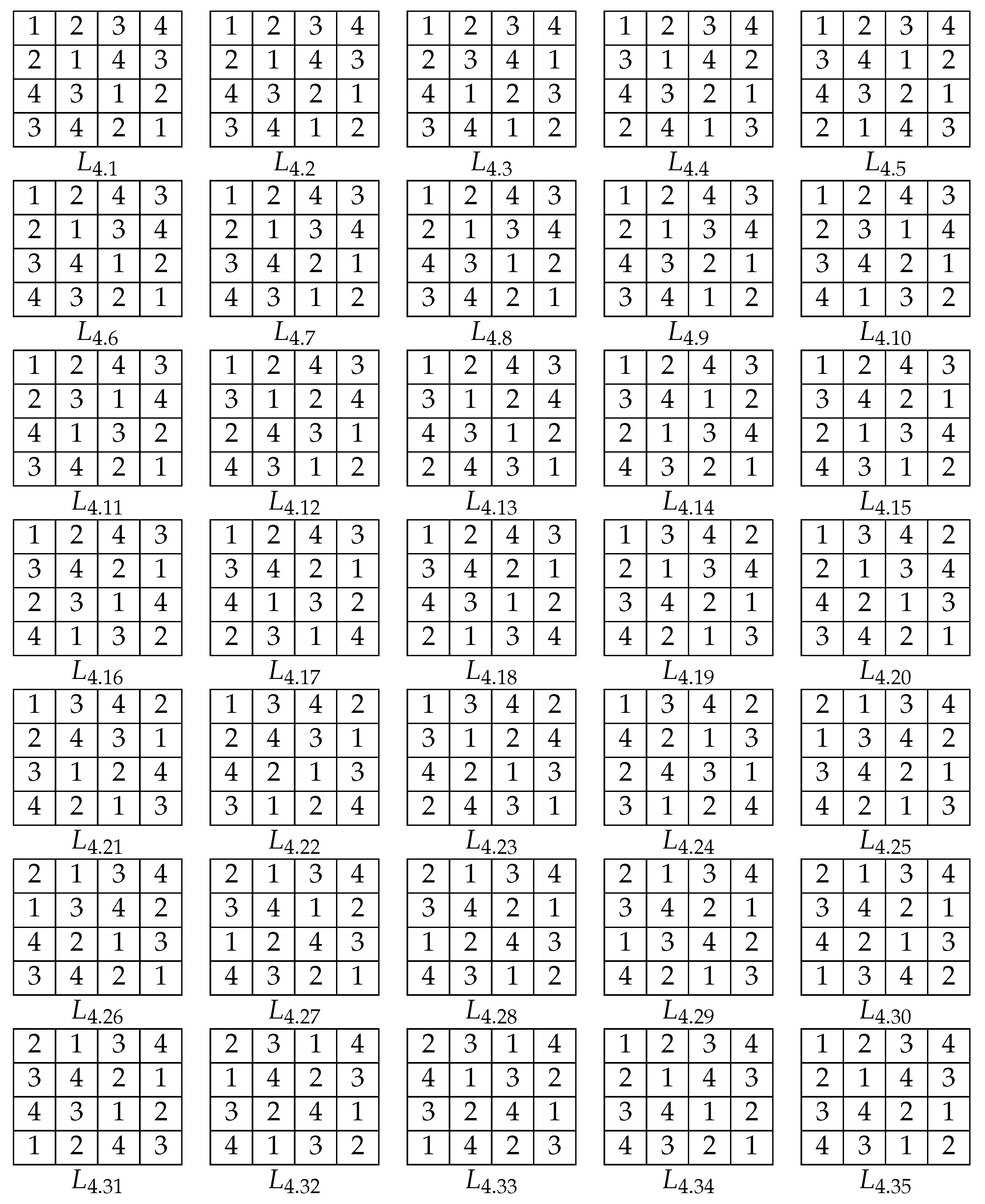
Lemma 1 establishes the existing relationship among image patterns arisen from Latin squares and the distribution into isomorphism classes of the latter. This section focuses on a particular subset of image patterns, which may enable one to determine, even from a visual way, whether two Latin squares are not isomorphic. In this regard, let m, n, r and s be four positive integers such that $s\le n$. We define the s-standard $r\times m$ image pattern associated to a Latin square $L\in {\mathcal{L}}_{n;n^2}$ as ${\mathcal{P}}_{r,m;s}\left(L\right):={\mathcal{P}}_{S,T}\left(L\right)$, where S is the constant $(r-1)$-tuple $(s,\dots ,s)$ and T is the constant plaintext $s\dots s$ of length m. We call it constant if all its entries coincide. In addition, we term the set $\{{\mathcal{P}}_{r,m;s}:s\in \left[n\right]\}$ the standard set of $r\times m$ image patterns associated to L. From Lemma 1, if the standard sets of $r\times m$ image patterns associated to two Latin squares do not coincide up to permutation of symbols, then these Latin squares are not isomorphic. As such, the analysis of standard sets turns out to be of particular interest for distinguishing non-isomorphic Latin squares even from a simple visual way.

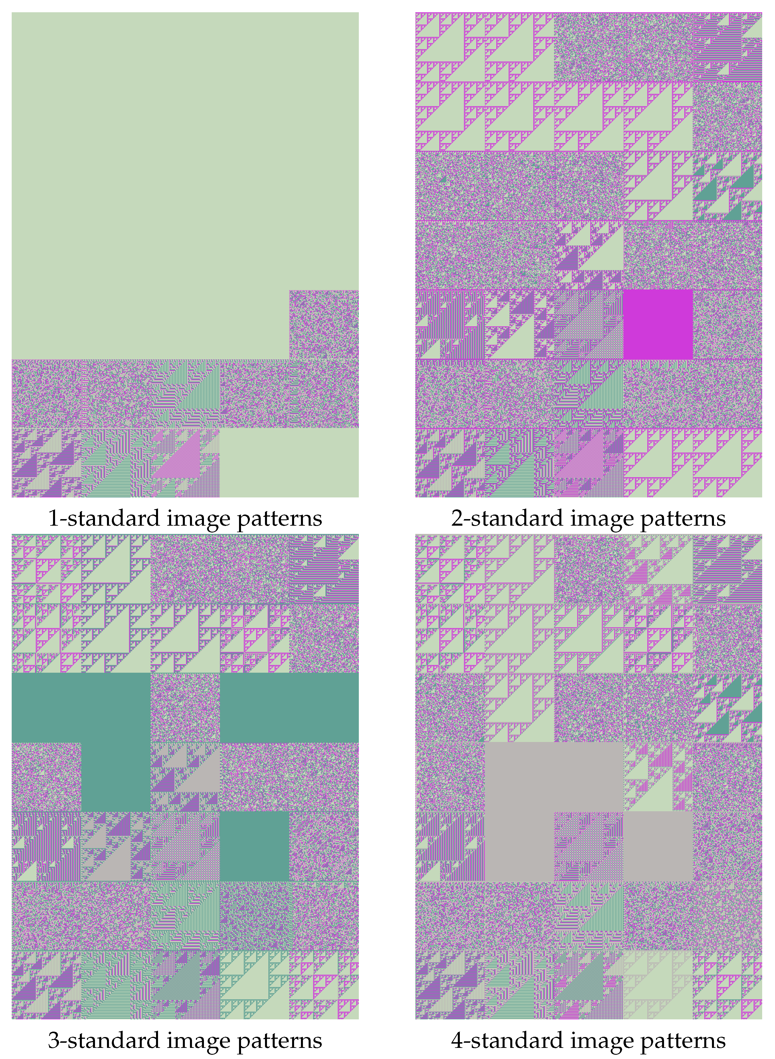
To illustrate this fact, let us focus on the standard $90\times 90$ image patterns associated to each one of the 35 isomorphism classes in which the set of Latin squares of order $n=4$ is distributed. (The case $n=3$ was already analyzed by Falcón, R.M. et al. [36].) A representative of each one of these classes is described in Figure 1. Their respective standard image patterns are shown in Figure 2. It is formed by four collages in form of $7\times 5$ arrays. They were created by means of the commands Colorize and ImageAssemble in Wolfram Mathematica [47]. Each standard image pattern is represented as a pixel array so that each symbol is uniquely replaced by a color within a given palette of four colors. Each cell within any of these arrays constitutes the corresponding standard image pattern that is associated to the Latin square described at the same position within Figure 1. The union of the four standard images patterns associated to such a Latin square constitutes its standard set of $90\times 90$ image patterns.

These standard sets can be distributed according to the following classification.

• Constant standard image patterns.
  A simple observation of the monochromatic cells in Figure 2 enables us to determine this type of standard image patterns. Notice that the s-standard image pattern of a Latin square $L=\left(l_{i,j}\right)$ is constant if and only if $l_{s,s}=s$.
• Fractal standard image patterns.
  From a simple visual inspection, one can observe that some of the cells in Figure 2 have a fractal character. It is the case, for instance, of the 2-standard image pattern associated to the Latin square $L_{4.1}$.
• Non-fractal standard image patterns.
  The remaining cells do not have a clear fractal character. Their spectrum goes from what one may label as a chaotic behavior (see, for instance, the 2-standard image pattern associated to $L_{4.30}$) to a shadow of fractal behavior (see, for instance, the 2-standard image pattern related to $L_{4.11}$). In any case, we do not distinguish in this paper the fractal gradation of the image patterns under consideration.

Table 1. Number of constant ($♯{\mathrm{cs}}_i$), fractal ($♯{\mathrm{fs}}_i$) and non-fractal ($♯{\mathrm{nfs}}_i$) $90\times 90$ standard image patterns associated to the 35 representatives ($L_{4.i}$) described in Figure 1.

i	$♯{\mathbf{cs}}_{\mathit{i}}$	$♯{\mathbf{fs}}_{\mathit{i}}$	i	$♯{\mathbf{cs}}_{\mathit{i}}$	$♯{\mathbf{fs}}_{\mathit{i}}$	i	$♯{\mathbf{cs}}_{\mathit{i}}$	$♯{\mathbf{fs}}_{\mathit{i}}$
1	1	3	13	1	0	25	0	0
2	1	3	14	2	1	26	0	0
3	1	0	15	2	2	27	0	0
4	1	1	16	1	0	28	0	4
5	1	3	17	3	0	29	0	0
6	1	3	18	2	2	30	0	0
7	1	3	19	1	1	31	0	4
8	1	3	20	1	0	32	0	4
9	1	3	21	1	3	33	0	4
10	1	0	22	2	2	34	1	3
11	2	0	23	1	3	35	1	3
12	2	1	24	4	0

shows the values $♯{\mathrm{cs}}_i$ and $♯{\mathrm{fs}}_i$ corresponding, respectively, to the number of constant and fractal standard image patterns within the standard set of $90\times 90$ image patterns of the Latin square $L_{4.i}$ in Figure 1, for every positive integer $i\le 35$. As introduced above, the number of its non-fractal standard image patterns would be, therefore, $4-♯{\mathrm{cs}}_i-♯{\mathrm{fs}}_i$. Notice that the first parameter characterizes the isomorphism classes having $L_{4.17}$ and $L_{4.24}$ as representatives, which are the only ones containing respectively three and four constant standard image patterns.

In addition, the representative $L_{4.11}$ is the only one that is associated to two constant and two non-fractal standard image patterns. The remaining standard sets are not easy to distinguish visually, particularly those ones containing non-fractal standard image patterns. An alternative approach to deal with these cases consists of making use of different techniques concerning computational algebraic geometry [36].

Let us define the affine algebraic set associated to the s-standard $r\times m$ image pattern ${\mathcal{P}}_{r,m;s}\left(L\right)=\left(p_{i,j}\right)$ of a Latin square $L\in {\mathcal{L}}_{n;n^2}$ in the multivariate polynomial ring $\mathbb{Q}\left[\{x_1,\dots ,x_n\}\right]$ as the set of zeros of the binomial ideal

$$I\left({\mathcal{P}}_{r,m;s}\left(L\right)\right):=\langle x_{p_{i,j-1}}{x}_{p_{i-1,j}}-x_{p_{i,j}}:1<i\le r,1<j\le m\rangle .$$

From (1) and (2), it is $I\left({\mathcal{P}}_{r,m;s}\left(L\right)\right)\subseteq I\left(L\right)$ and hence, ${\mathcal{V}}_{\mathbb{Q}}\left(I\left(L\right)\right)\subseteq {\mathcal{V}}_{\mathbb{Q}}\left(I\left({\mathcal{P}}_{r,m;s}\left(L\right)\right)\right)$.

Example 6.

Let us consider the Latin square $L_{4.12}$ described in Figure 1 and the multivariate polynomial ring $\mathbb{C}\left[\{x_1,x_2,x_3,x_4\}\right]$. The reduced Gröbner basis associated to the binomial ideal $I\left(L_{4.12}\right)$ is the subset

$$\left\{x_1-x_4,x_2-x_4,x_3-x_4,x_4^2-x_2\right\}\subset I\left(L_{4.12}\right),$$

whereas that one associated to the ideal $I\left({\mathcal{P}}_{90,90;4}\left(L_{4.12}\right)\right)$ is the subset

$$\left\{x_1-x_2,x_3-x_4,x_2^2-x_2,x_2{x}_4-x_4,x_4^2-x_2\right\}\subset I\left({\mathcal{P}}_{90,90;4}\left(L\right)\right).$$

Hence, both ideals are zero-dimensional. Their associated affine algebraic sets are

$${\mathcal{V}}_{\mathbb{C}}\left(I\left(L_{4.12}\right)\right)=\{(0,0,0,0),(1,1,1,1)\}$$

and

$${\mathcal{V}}_{\mathbb{C}}\left(I\left({\mathcal{P}}_{90,90;4}\left(L_{4.12}\right)\right)\right)=\{(0,0,0,0),(1,1,1,1),(1,1,-1,-1)\}.$$

Of course, if the standard sets of $r\times m$ image patterns associated to two Latin squares of the same order n coincide, up to permutation of symbols, then the multisets formed by the respective cardinalities of each one of the n affine algebraic sets related to their standard image patterns must also coincide. In particular, from Lemma 1, these multisets coincide for any two isomorphic Latin squares. To illustrate these aspects,

Table 2. Cardinalities ($♯V_{i,s}$) of the affine algebraic set ${\mathcal{V}}_{\mathbb{Q}}\left(I\left({\mathcal{P}}_{90,90;s}\left(L_{4.i}\right)\right)\right)$, for all positive integers $i\le 35$ and $s\le 4$.

i	$♯{\mathit{V}}_{\mathit{i},1}$	$♯{\mathit{V}}_{\mathit{i},2}$	$♯{\mathit{V}}_{\mathit{i},3}$	$♯{\mathit{V}}_{\mathit{i},4}$	i	$♯{\mathit{V}}_{\mathit{i},1}$	$♯{\mathit{V}}_{\mathit{i},2}$	$♯{\mathit{V}}_{\mathit{i},3}$	$♯{\mathit{V}}_{\mathit{i},4}$
1	∞	∞	3	3	19	∞	2	2	2
2	∞	∞	3	3	20	∞	2	2	2
3	∞	2	2	2	21	∞	2	2	2
4	∞	2	2	2	22	∞	2	2	∞
5	∞	2	2	2	23	∞	2	2	2
6	∞	∞	3	3	24	∞	∞	∞	∞
7	∞	∞	3	3	25	2	2	2	2
8	∞	∞	3	3	26	2	2	2	2
9	∞	∞	3	3	27	2	2	2	2
10	∞	2	2	2	28	2	2	2	2
11	∞	2	∞	2	29	2	2	2	2
12	∞	2	∞	3	30	2	2	2	2
13	∞	2	2	2	31	2	2	2	2
14	∞	3	∞	2	32	2	2	2	2
15	∞	2	∞	2	33	2	2	2	2
16	∞	2	2	2	34	∞	∞	∞	∞
17	∞	2	∞	∞	35	∞	∞	5	5
18	∞	2	2	∞

shows all these cardinalities for the standard image patterns described in Figure 2. It is so that there exist ten isomorphism classes of Latin squares of order four that are related to the multiset $\{2,2,2,\infty \}$, nine classes to $\{2,2,2,2\}$, six classes to $\{3,3,\infty ,\infty \}$, four classes to $\{2,2,\infty ,\infty \}$, two classes to $\{2,3,\infty ,\infty \}$ and another two classes to $\{\infty ,\infty ,\infty ,\infty \}$. Moreover, there are two isomorphism classes that are characterized by their respective multisets. Their representatives are the Latin squares $L_{4.17}$ and $L_{4.35}$, which are, respectively, associated to the multisets $\{2,\infty ,\infty ,\infty \}$ and $\{5,5,\infty ,\infty \}$. In addition, notice that the combination of Table 1 and Table 2 characterizes the isomorphism class having the Latin square $L_{4.34}$ as its representative.

To facilitate the recognition and analysis of similar standard sets for distinguishing non-isomorphic Latin squares of the same order n, even from a simple visual observation, one may focus on those ones having exactly the same positive number of fractal standard image patterns, as well as the same number of constant standard image patterns and the same multisets of cardinalities of their related affine algebraic sets. Let us illustrate this fact with the case $n=4$, by means of the values in Table 1 and Table 2 concerning the standard sets described in Figure 2.

• The standard sets of both Latin squares $L_{4.4}$ and $L_{4.19}$ are the only ones having exactly one constant and one fractal standard image patterns. To prove that they are indeed non-isomorphic, it is enough to focus on their fractal standard image patterns. In both cases, they correspond to their respective 4-standard image patterns, for which a simple visual observation of Figure 2 enables us to ensure that they are not coincident, even after a permutation of colors.
• A similar reasoning may be done for the standard sets of the Latin squares $L_{4.15}$, $L_{4.18}$ and $L_{4.22}$, which are the only ones having two constant and two fractal standard image patterns. A simple observation of Figure 2 enables us to ensure that their respective sets of fractal standard image patterns are pairwise distinct, even after a permutation of colors.
• The same happens with the four Latin squares $L_{4.28}$, $L_{4.31}$, $L_{4.32}$ and $L_{4.33}$.
• A more interesting case is that one concerning the eleven isomorphism classes whose respective standard sets contain exactly one constant and three fractal standard image patterns. Table 2 partitions them into four disjoint subsets. Two of them have already been characterized by these parameters. They correspond to the Latin squares $L_{4.34}$ and $L_{4.35}$. The other two subsets are the following ones.

  −

  The subset formed by the three Latin squares $L_{4.5}$, $L_{4.21}$ and $L_{4.23}$. Similarly to the previous cases, their standard sets are visually characterized in a simple way.

  −

  The subset formed by the six Latin squares $L_{4.1}$, $L_{4.2}$, $L_{4.6}$, $L_{4.7}$, $L_{4.8}$ and $L_{4.9}$. Here, the visual distinction of their fractal standard image patterns in Figure 2 is not so evident. It is so that all their 2-standard image patterns coincide and a much more detailed observation of their 3- and 4-standard sets is required for ensuring that their standard sets are pairwise distinct.

• A detailed observation is also required for distinguishing visually the standard sets of the Latin squares $L_{4.12}$ and $L_{4.14}$, both of them containing exactly two constant and one fractal standard image pattern. More specifically, it may be checked (either visually or by making use of Definition 2) that the second row of the fractal standard image pattern of $L_{4.12}$ contains all the four colors or symbols under consideration, whereas that one of $L_{4.14}$ only contains two of them.

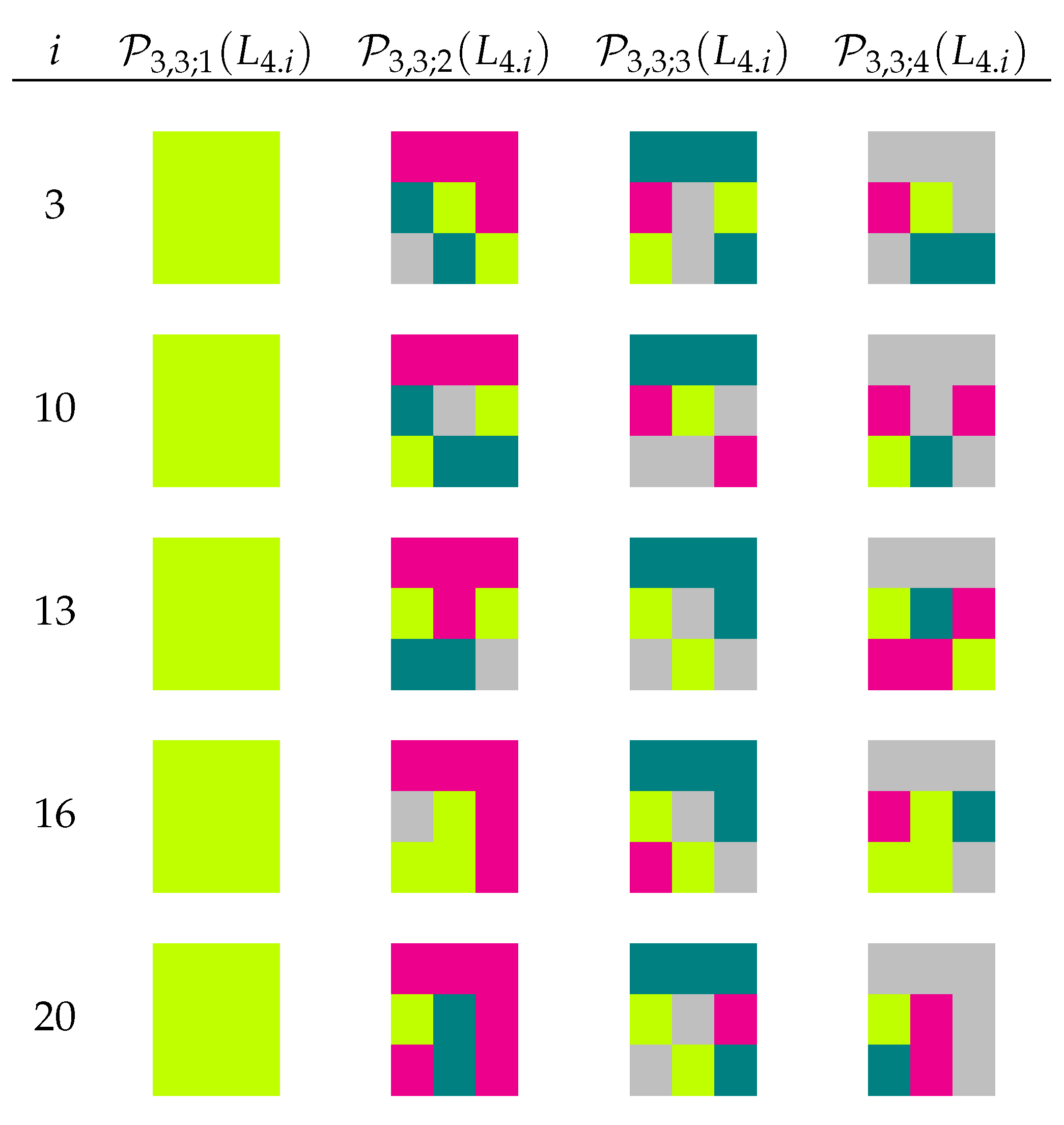
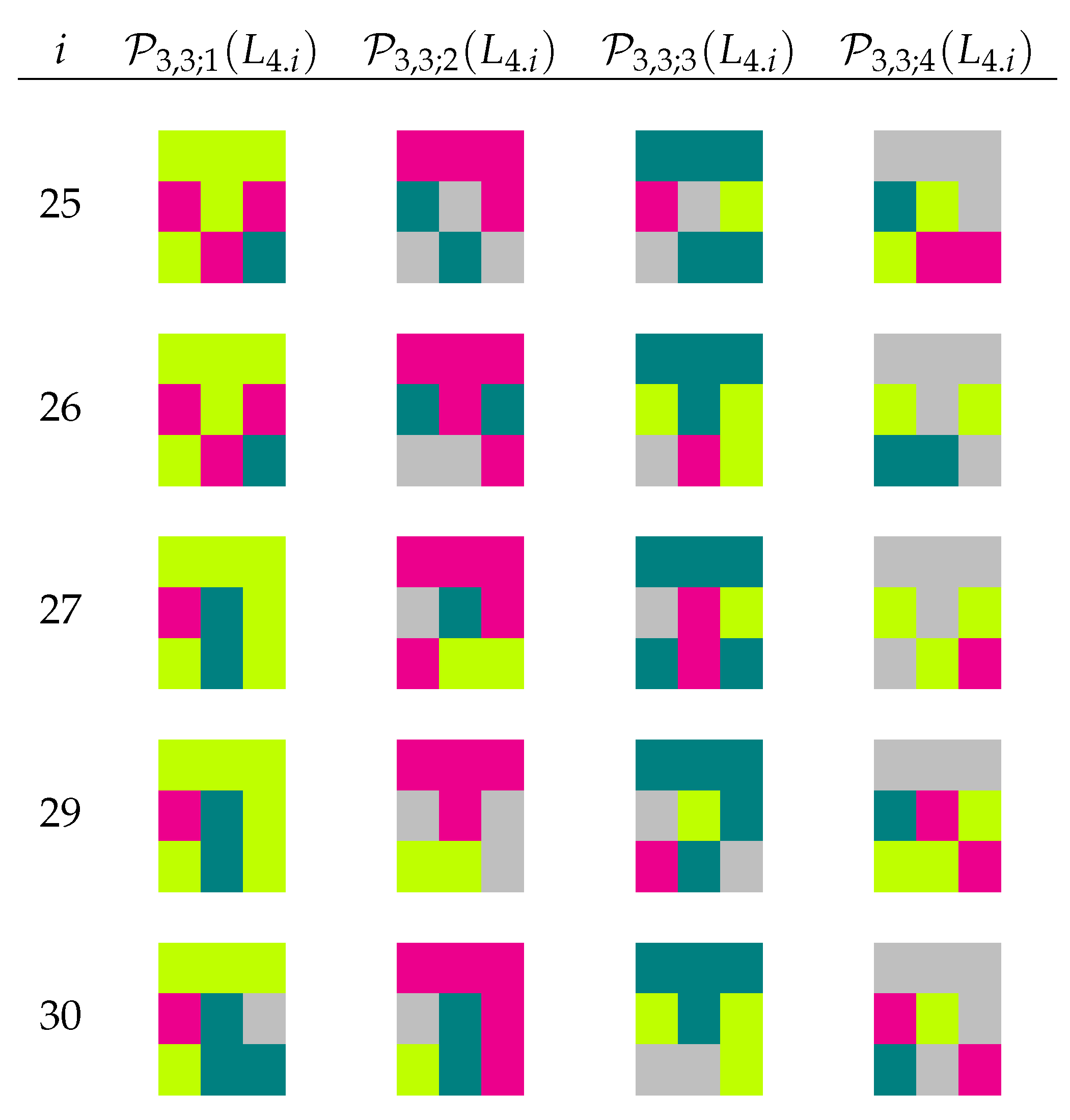
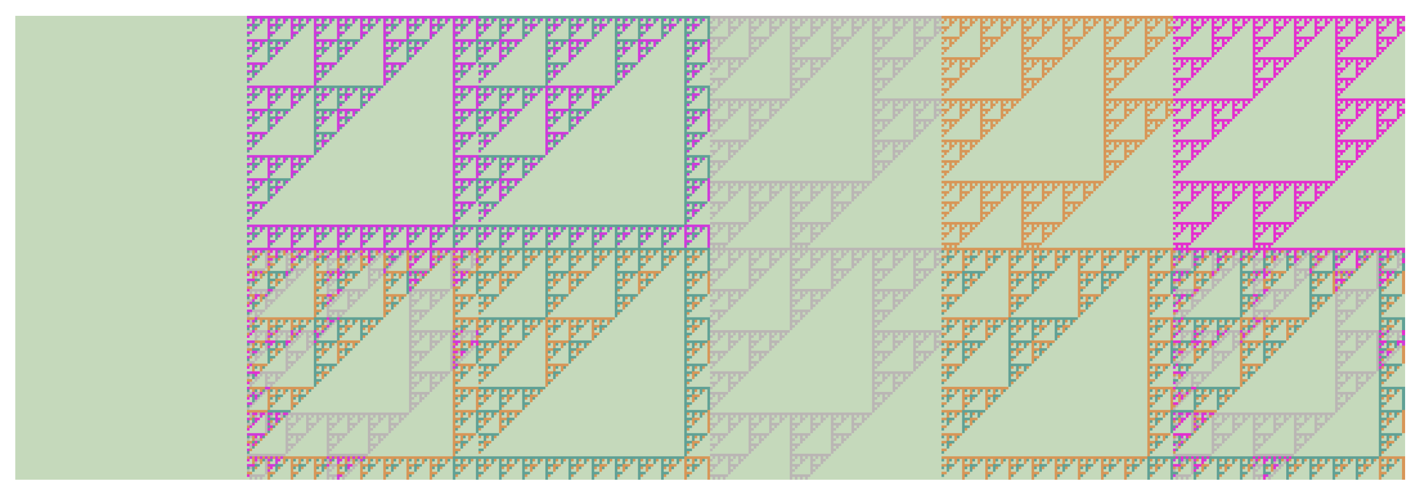
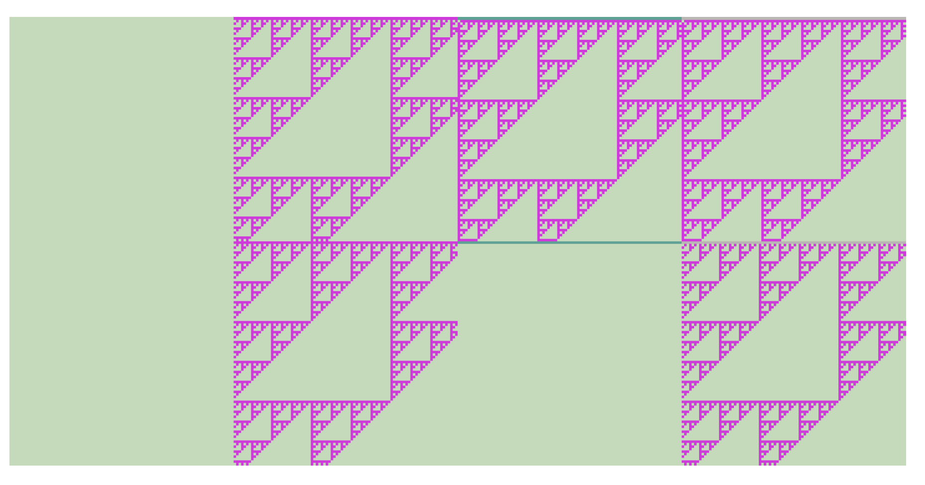
None of the standard sets of the remaining ten isomorphism classes contains fractal standard image patterns, which makes much more difficult their visual distinction. According to their respective parameters, they can be partitioned into the following two sets.

• The subset formed by the five Latin squares $L_{4.3}$, $L_{4.10}$, $L_{4.13}$, $L_{4.16}$ and $L_{4.20}$. Their standard sets contains exactly one constant standard image patterns. Notice that $L_{4.3}$ and $L_{4.13}$ are respective transpose of $L_{4.10}$ and $L_{4.20}$.
• The subset formed by the five Latin squares $L_{4.25}$, $L_{4.26}$, $L_{4.27}$, $L_{4.29}$ and $L_{4.30}$. None of their standard sets contain constant standard image patterns.

A possible approach to analyze the non-fractal standard image patterns of both subsets is reducing their dimension, which is equivalent to zoom in to the left upper corner of the original standard image patterns. Based on this approach, it is simply verified from the results in Figure 3 and Figure 4 that the standard sets of $3\times 3$ image patterns associated to these two subsets are pairwise distinct, even allowing a possible permutation of symbols.

4. A Computational Algebraic Geometry Approach to Deal with Being Either Partial Transpose or Partial Isotopic

We show in Section 3 how the computation of isomorphism invariants concerning affine algebraic sets based on a set of Latin squares plays a fundamental role in the recognition and analysis of their related image patterns. Apart from these invariants, the existence of certain equivalence relations among partial Latin squares of the same order and weight is also known [36], which give rise to the same or isomorphic affine algebraic sets. It is the case of being partial transpose and being P-partial isotopic, for some subset $P\subset \left[n\right]\times \left[n\right]\times \left[n\right]$ (see Lemma 2 and Proposition 1). Let us finish this paper by showing how computational algebraic geometry is also an interesting approach to deal with both equivalence relations. To this end, let us introduce a pair of ideals within a multivariate polynomial ring, whose respective affine algebraic sets are respectively identified with the set of partial Latin squares that are partial transpose of another given partial Latin square, and the set of partial isotopisms between two partial Latin squares.

Firstly, for each positive integer n, we consider the set of $n^3$ variables

$$X_n^{\mathrm{PT}}:=\{x_{ijk}:1\le i,j,k\le n\}.$$

Then, for each positive integer $m\le n^2$, it is known [18] (see also [27,29] for a pair of first approaches in this regard) that the set ${\mathcal{L}}_{n;m}$ is uniquely identified with the set of zeros of the affine algebraic set of the following ideal in $\mathbb{Q}\left[X_n^{\mathrm{PT}}\right]$.

$$\begin{array}{cc}\hfill I_{n;m}:=& 〈x_{ijk}^2-x_{ijk}:1\le i,j,k\le n〉\hfill \\ \hfill & +〈x_{ijk}{x}_{i^{\prime }jk}:1\le i,i^{\prime },j,k\le n,i<i^{\prime }〉\hfill \\ \hfill & +〈x_{ijk}{x}_{i{j}^{\prime }k}:1\le i,j,j^{\prime },k\le n,j<j^{\prime }〉\hfill \\ \hfill & +〈x_{ijk}{x}_{ij{k}^{\prime }}:1\le i,j,k,k^{\prime }\le n,k<k^{\prime }〉\hfill \\ \hfill & +〈m-\sum _{i,j,k=1}^n{x}_{ijk}〉.\hfill \end{array}$$

Let us recall here that the sum of two ideals I and J is the ideal $I+J=\{i+j:i\in I,j\in J\}$. Each addend constitutes a subideal of the resulting ideal. Hence, our ideal $I_n$ is the sum of four subideals. The first one implies that any zero of $I_n$ is of the form $(a_{111},\dots ,a_{nnn})\in {\{0,1\}}^{n^3}$. The remaining subideals imply that this zero is uniquely identified with a partial Latin square $L=\left(l_{i,j}\right)\in {\mathcal{L}}_{n;m}$ such that $l_{i,j}=k\in \left[n\right]$ if and only if $a_{ijk}=1$.

Now, for each partial Latin square $L\in {\mathcal{L}}_{n;m}$, let us define the following ideal in the multivariate polynomial ring $\mathbb{Q}\left[X_n^{\mathrm{PT}}\right]$.

$$\begin{array}{cc}\hfill I_{\mathrm{PT}}\left(L\right):=I_{n;m}+& 〈(x_{ijk}-1)·(x_{jik}-1):(i,j,k)\in \mathrm{Ent}\left(L\right)〉\hfill \\ \hfill & 〈x_{ijk},x_{jik}:\{(i,j,k),(j,i,k)\}\cap \mathrm{Ent}\left(L\right)=\varnothing ,1\le i,j,k\le n〉.\hfill \end{array}$$

Lemma 3.

The set of partial Latin squares that are partial transpose to a partial Latin square $L\in {\mathcal{L}}_{n;m}$ is uniquely identified with the affine algebraic set of the ideal $I_{\mathrm{PT}}\left(L\right)$.

Proof. 

Let $(a_{111},\dots ,a_{nnn})\in {\{0,1\}}^{n^3}$ be a zero of the ideal $I_{\mathrm{PT}}\left(L\right)$. In particular, it must be a zero of the ideal $I_{n;m}$ and, hence, it is uniquely identified with a partial Latin square $L^{\prime }\in {\mathcal{L}}_{n;m}$ such that $(i,j,k)\in \mathrm{Ent}\left(L^{\prime }\right)$ if and only if $a_{ijk}=1$. From the subideal

$$〈(x_{ijk}-1)·(x_{jik}-1):(i,j,k)\in \mathrm{Ent}\left(L\right)〉,$$

we have that, if $(i,j,k)\in \mathrm{Ent}\left(L\right)$, then either $a_{ijk}=1$ or $a_{jik}=1$. As a consequence, if $(i,j,k)\in \mathrm{Ent}\left(L\right)\backslash \mathrm{Ent}\left(L^{\prime }\right)$, then $(j,i,k)\in \mathrm{Ent}\left(L^{\prime }\right)$.

Now, let $(i,j,k)\in \mathrm{Ent}\left(L^{\prime }\right)\backslash \mathrm{Ent}\left(L\right)$. In particular, it must be $a_{ijk}=1$. If $(j,i,k)\notin \mathrm{Ent}\left(L\right)$, then the last subideal describing $I_{\mathrm{PT}}\left(L\right)$ implies that $a_{ijk}=0$, which is a contradiction. Hence, $(j,i,k)\in \mathrm{Ent}\left(L\right)$. Therefore, the partial Latin squares L and $L^{\prime }$ are partial transpose of each other. □

Example 7.

Let us consider the partial Latin square

$$L\equiv \boxed{\begin{array}{ccc}1& 2& \\ 3& & 1\\ 2& & 3\end{array}}\in {\mathcal{L}}_{3;5}.$$

The reduced Gröbner basis of the ideal $I_{\mathrm{PT}}\left(L\right)\subset \mathbb{Q}\left[X_3^{\mathrm{PT}}\right]$ is the subset

$$\begin{array}{cc}& \{x_{321}^2-x_{321},x_{312}^2-x_{312},x_{231}+x_{321}-1,x_{213}-x_{312},x_{212}+x_{312}-1\}\hfill \\ \cup \hfill & \{x_{132}+x_{312}-1,x_{123}+x_{312}-1,x_{122}-x_{312},x_{333}-1,x_{111}-1,x_{332},x_{331},x_{323}\}\hfill \\ \cup \hfill & \{x_{322},x_{313},x_{311},x_{233},x_{232},x_{223},x_{222},x_{221},x_{211},x_{133},x_{131},x_{121},x_{113},x_{112}\}\subset I_{\mathrm{PT}}\left(L\right).\hfill \end{array}$$

Hence, the affine algebraic set of the ideal $I_{\mathrm{PT}}\left(L\right)$ is formed by four points that are uniquely associated to L and the following three partial Latin squares.

$$\boxed{\begin{array}{ccc}1& 3& 2\\ 2& & 1\\ & & 3\end{array}}\boxed{\begin{array}{ccc}1& 3& 2\\ 2& & \\ & 1& 3\end{array}}\boxed{\begin{array}{ccc}1& 2& \\ 3& & \\ 2& 1& 3\end{array}}$$

From Lemma 3, computational algebraic geometry can be used for distributing partial Latin squares of the same order n according to the equivalence relation of being partial transpose. The following result establishes the computational cost that is required to this end in case of being $n\ge 2$. (The case $n=1$ is trivial.)

Theorem 2.

Let $L\in {\mathcal{L}}_n$, with $n\ge 2$. The arithmetic complexity of computing the reduced Gröbner basis of the ideal $I_{\mathrm{PT}}\left(L\right)$ over the field $\mathbb{Q}$ is bounded above by

$${\left(\frac{2\left(3n^3-3n^2+9n+\left|\mathrm{Ent}\left(L\right)\right|\right)+{\alpha }_1+2{\alpha }_2+1}{3n^3-3n^2+9n+\left|\mathrm{Ent}\left(L\right)\right|+{\alpha }_1+2{\alpha }_2+1}\right)}^{n^3}<2^{n^3},$$

where

$${\alpha }_1:=\left|\left\{(i,i,k)\notin \mathrm{Ent}\left(L\right):1\le i,k\le n\right\}\right|$$

and

$${\alpha }_2:=\left|\left\{(i,j,k):\left\{(i,j,k),(j,i,k)\right\}\cap \mathrm{Ent}\left(L\right)=\varnothing ,1\le i<j\le n,1\le k\le n\right\}\right|.$$

Proof. 

The ideal $I_{\mathrm{PT}}\left(L\right)$ is zero-dimensional, because ${\mathcal{V}}_{\mathbb{Q}}\left(I_{\mathrm{PT}}\left(L\right)\right)\subset {\{0,1\}}^{n^3}$. Thus, the result holds from Theorem 1 and the generators of this ideal, whose coefficients have all of them size one. To see it,

Table 3. Study of the generators of the ideal $I_{\mathrm{PT}}\left(L\right)$.

Generator Type	Maximum Degree	Number of Generators
$x_{ijk}^2-x_{ijk}$	2	$3n$
$x_{ijk}{x}_{i^{\prime }jk}$	2	$n^3-n^2+2n$
$x_{ijk}{x}_{i{j}^{\prime }k}$	2	$n^3-n^2+2n$
$x_{ijk}{x}_{ij{k}^{\prime }}$	2	$n^3-n^2+2n$
$m-{\sum }_{i,j,k=1}^n{x}_{ijk}$	1	1
$(x_{ijk}-1)·(x_{jik}-1)$	2	$\left|\mathrm{Ent}\right(L\left)\right|$
$x_{iik}$	1	${\alpha }_1$
$x_{ijk}$ (with $i\ne j$)	1	$2{\alpha }_2$

shows the maximum degree of each one of these generators, together with the number of generators of each type. Then, the result follows because, from Theorem 1, the required arithmetic complexity is bounded above by the maximum value between

$$n^3\left(\left(3n^3-3n^2+9n+\left|\mathrm{Ent}\left(L\right)\right|\right)\left(\genfrac{}{}{0pt}{}{n^3+2}{n^3}\right)+({\alpha }_1+2{\alpha }_2+1)(n^3+1)\right)$$

and

$${\left(\frac{2\left(3n^3-3n^2+9n+\left|\mathrm{Ent}\left(L\right)\right|\right)+{\alpha }_1+2{\alpha }_2+1}{3n^3-3n^2+9n+\left|\mathrm{Ent}\left(L\right)\right|+{\alpha }_1+2{\alpha }_2+1}\right)}^{n^3}.$$

 □

A computational algebraic geometry approach can also be described in the case of dealing with the equivalence relation of being P-partial isotopic, for some subset $P\subset \left[n\right]\times \left[n\right]\times \left[n\right]$. It follows similarly to the approach concerning the equivalence relation of being isotopic, which was described in (Theorem 13, [18]). To this end, for each positive integer n, let us consider the set of $3n^2$ variables

$$X_n^{\mathrm{PI}}:=\left\{x_{ij},y_{ij},z_{ij}:1\le i,j\le n\right\}.$$

Then, for each pair of partial Latin squares $L_1=\left(l_{i,j}\right)$ and $L_2=\left(l_{i,j}^{\prime }\right)$ in the set ${\mathcal{L}}_{n;m}$, let us define the following ideal in the multivariate polynomial ring $\mathbb{Q}\left[X_n^{\mathrm{PI}}\right]$.

$$\begin{array}{cc}\hfill I_{\mathrm{PI}}(L_1,L_2):=& 〈x_{ij}^2-x_{ij},y_{ij}^2-y_{ij},z_{ij}^2-z_{ij}:1\le i,j\le n〉\hfill \\ \hfill +& 〈1-\sum _{j=1}^n{x}_{ij},1-\sum _{j=1}^n{x}_{ji}:1\le i\le n〉\hfill \\ \hfill +& 〈1-\sum _{j=1}^n{y}_{ij},1-\sum _{j=1}^n{y}_{ji}:1\le i\le n〉\hfill \\ \hfill +& 〈1-\sum _{j=1}^n{z}_{ij},1-\sum _{j=1}^n{z}_{ji}:1\le i\le n〉\hfill \\ \hfill +& 〈x_{i{i}^{\prime }}{y}_{j{j}^{\prime }}(z_{l_{i,j}{l}_{i^{\prime },j^{\prime }}^{\prime }}-1):1\le i,i^{\prime },j,j^{\prime },l_{i,j},l_{i^{\prime },j^{\prime }}^{\prime }\le n,\mathrm{with}{l}_{i,j}\ne l_{i,j}^{\prime }〉\hfill \\ \hfill +& 〈x_{i{i}^{\prime }}{y}_{j{j}^{\prime }}:1\le i,i^{\prime },j,j^{\prime }\le n,l_{i,j}=\varnothing \notin \left\{l_{i,j}^{\prime },l_{i^{\prime },j^{\prime }}^{\prime }\right\}〉\hfill \\ \hfill +& 〈x_{i{i}^{\prime }}{y}_{j{j}^{\prime }}:1\le i,i^{\prime },j,j^{\prime }\le n,l_{i,j}=l_{i,j}^{\prime }=\varnothing \ne l_{i^{\prime },j^{\prime }}^{\prime }〉\hfill \\ \hfill +& 〈x_{i{i}^{\prime }}{y}_{j{j}^{\prime }}:1\le i,i^{\prime },j,j^{\prime }\le n,l_{i,j}\ne \varnothing =l_{i^{\prime },j^{\prime }}^{\prime }\mathrm{and}{l}_{i,j}\ne l_{i,j}^{\prime }〉.\hfill \end{array}$$

Lemma 4.

Two partial Latin squares $L_1$ and $L_2$ in the set ${\mathcal{L}}_{n;m}$ are P-partial isotopic, for some subset $P\subset \left[n\right]\times \left[n\right]\times \left[n\right]$, if and only if the affine algebraic set of the ideal $I_{\mathrm{PI}}(L_1,L_2)$ is non-empty.

Proof. 

Let us suppose the existence of a zero $(a_{11},\dots ,a_{nn},b_{11},\dots ,b_{nn},c_{11},\dots ,c_{nn})\in {\{0,1\}}^{3n^2}$ of the ideal $I_{\mathrm{PI}}(L_1,L_2)$. The first three subideals describing this ideal imply that this zero is uniquely related to an isotopism $(f,g,h)\in S_n^3$ such that, for each pair of positive integers $i,j\le n$, the following assertions hold.

• $f\left(i\right)=j$ if and only if $a_{ij}=1$.
• $g\left(i\right)=j$ if and only if $b_{ij}=1$.
• $h\left(i\right)=j$ if and only if $c_{ij}=1$.

The fourth subideal implies that this isotopism constitutes a one-to-one map from $\mathrm{Ent}\left(L_1\right)\backslash \mathrm{Ent}\left(L_2\right)$ to $\mathrm{Ent}\left(L_2\right)$. The fifth one implies that, if the cell $(i,j)$ is empty in $L_1$ but not in $L_2$, then the former cannot be mapped to a non-empty cell in $L_2$. Further, the sixth subideal implies that, if the cell $(i,j)$ is empty in both $L_1$ and $L_2$, then it cannot be mapped to a non-empty cell in $L_2$. Finally, the last subideal implies that, if the cell $(i,j)$ contains distinct symbols in $L_1$ and $L_2$, then it cannot be mapped to an empty cell in $L_2$. Under such assumptions, it is readily verified that the zero under consideration is uniquely identified with a P-partial isotopism from $L_1$ to $L_2$, where $P\subseteq \mathrm{Ent}\left(L_1\right)\cap \mathrm{Ent}\left(L_2\right)$. □

Example 8.

Let us consider the Latin squares $L_1$ and $L_3$ in Example 2. The reduced Gröbner basis of the ideal $I_{\mathrm{PI}}(L_1,L_3)\subset \mathbb{Q}\left[X_4^{\mathrm{PI}}\right]$ is the subset $\left\{1\right\}\subset I_{\mathrm{PI}}(L_1,L_3)$. Thus, the related affine algebraic set is empty and hence, no partial isotopism exists between $L_1$ and $L_3$.

Example 9.

Let us consider the partial Latin square $L_1$ and $L_2$ described in Example 3. The reduced Gröbner basis of the ideal $I_{\mathrm{PI}}(L_1,L_2)\subset \mathbb{Q}\left[X_4^{\mathrm{PI}}\right]$ is the subset

$$\begin{array}{cc}& \{z_{22}^2-z_{22},z_{21}+z_{22}-1,z_{12}+z_{22}-1,z_{11}-z_{22},z_{44}-1,z_{43},z_{42},z_{41},z_{34},z_{33}-1\}\hfill \\ \cup \hfill & \{z_{32},z_{31},z_{24},z_{23},z_{14},z_{13},y_{44},y_{43},y_{42},y_{41}-1,y_{34},y_{33},y_{32}-1,y_{31},y_{24}-1,y_{23}\}\hfill \\ \cup \hfill & \{y_{22},y_{21},y_{14},y_{13}-1,y_{12},y_{11},x_{44},x_{43},x_{42}-1,x_{41},x_{34},x_{33},x_{32},x_{31}-1,x_{24}\}\hfill \\ \cup \hfill & \{x_{23}-1,x_{22},x_{21},x_{14}-1,x_{13},x_{12},x_{11}\}\subset I_{\mathrm{PI}}(L_1,L_2).\hfill \end{array}$$

Hence, the affine algebraic set of the ideal $I_{\mathrm{PI}}(L_1,L_2)$ is formed by two points that are uniquely associated to the isotopisms $\left(\right(1423),(1324),(12\left)\right)$ and $\left(\right(1423),(1324),\mathrm{Id})$ in $S_4^3$. Both of them constitute P-partial isotopisms from $L_1$ to $L_2$, where $P=\mathrm{Ent}\left(L_1\right)\cap \mathrm{Ent}\left(L_2\right)$.

From Lemma 4, computational algebraic geometry can be used for distributing partial Latin squares according to the equivalence relation of being P-partial isotopic, for some subset $P\subset \left[n\right]\times \left[n\right]\times \left[n\right]$. The following result establishes the computational cost that is required to this end in case of being $n>2$. (The case $n=1$ is trivial.)

Theorem 3.

Let $L_1$ and $L_2$ be two partial Latin squares in ${\mathcal{L}}_n$, with $n\ge 2$. The arithmetic complexity of computing the reduced Gröbner basis of the ideal $I_{\mathrm{PI}}(L_1,L_2)$ over the field $\mathbb{Q}$ is bounded above by

$${\left(\frac{3{\beta }_1+2(3n^2+{\beta }_2+{\beta }_3+{\beta }_4)+6n}{3n^2+6n+{\beta }_1+{\beta }_2+{\beta }_3+{\beta }_4}\right)}^{3n^2}<3^{3n^2},$$

where

$${\beta }_1:=\left|\left\{(i,i^{\prime },j,j^{\prime })\in \left[n\right]\times \left[n\right]\times \left[n\right]\times \left[n\right]:l_{i,j},l_{i^{\prime },j^{\prime }}^{\prime }\in \left[n\right],l_{i,j}\ne l_{i^{\prime },j^{\prime }}^{\prime }\right\}\right|,$$

$${\beta }_2:=\left|\left\{(i,i^{\prime },j,j^{\prime })\in \left[n\right]\times \left[n\right]\times \left[n\right]\times \left[n\right]:l_{i,j}=\varnothing \notin \left\{l_{i,j}^{\prime },l_{i^{\prime },j^{\prime }}^{\prime }\right\}\right\}\right|,$$

$${\beta }_3:=\left|\left\{(i,i^{\prime },j,j^{\prime })\in \left[n\right]\times \left[n\right]\times \left[n\right]\times \left[n\right]:l_{i,j}=l_{i,j}^{\prime }=\varnothing \ne l_{i^{\prime },j^{\prime }}^{\prime }\right\}\right|$$

and

$${\beta }_4:=\left|\left\{(i,i^{\prime },j,j^{\prime })\in \left[n\right]\times \left[n\right]\times \left[n\right]\times \left[n\right]:l_{i,j}\ne \varnothing =l_{i^{\prime },j^{\prime }}^{\prime }and{l}_{i,j}\ne l_{i,j}^{\prime }\right\}\right|$$

Proof. 

The ideal $I_{\mathrm{PI}}(L_1,L_2)$ is zero-dimensional, because ${\mathcal{V}}_{\mathbb{Q}}\left(I_{\mathrm{PI}}\left(L\right)\right)\subset {\{0,1\}}^{3n^2}$. Then, similarly to the proof of Theorem 2, the result holds from Theorem 1 and the generators of this ideal, whose coefficients have all of them size one. To see it,

Table 4. Study of the generators of the ideal $I_{\mathrm{PI}}(L_1,L_2)$.

Generator Type	Maximum Degree	Number of Generators
$x_{ij}^2-x_{ij}$	2	$n^2$
$y_{ij}^2-y_{ij}$	2	$n^2$
$z_{ij}^2-z_{ij}$	2	$n^2$
$1-{\sum }_{j=1}^n{x}_{ij}$	1	n
$1-{\sum }_{j=1}^n{x}_{ji}$	1	n
$1-{\sum }_{j=1}^n{y}_{ij}$	1	n
$1-{\sum }_{j=1}^n{y}_{ji}$	1	n
$1-{\sum }_{j=1}^n{z}_{ij}$	1	n
$1-{\sum }_{j=1}^n{z}_{ji}$	1	n
$x_{i{i}^{\prime }}{y}_{j{j}^{\prime }}(z_{l_{i,j}{l}_{i^{\prime },j^{\prime }}^{\prime }}-1)$	3	${\beta }_1$
$x_{i{i}^{\prime }}{y}_{j{j}^{\prime }}$	2	${\beta }_2+{\beta }_3+{\beta }_4$

shows the maximum degree of each one of these generators, together with the number of generators of each type. Then, the result holds because, from Theorem 2, the required arithmetic complexity is bounded above by the maximum value between

$$3n^2\left({\beta }_1\left(\genfrac{}{}{0pt}{}{3n^2+3}{3n^2}\right)+(3n^2+{\beta }_2+{\beta }_3+{\beta }_4)\left(\genfrac{}{}{0pt}{}{3n^2+2}{3n^2}\right)+6n(3n^2+1)\right).$$

and

$${\left(\frac{3{\beta }_1+2(3n^2+{\beta }_2+{\beta }_3+{\beta }_4)+6n}{3n^2+6n+{\beta }_1+{\beta }_2+{\beta }_3+{\beta }_4}\right)}^{3n^2}.$$

 □

5. Conclusions and Further Work

In this paper, we show the relevant role that computational algebraic geometry plays in the recognition and analysis of image patterns associated to Latin squares. To this end, we introduce the concepts of standard image pattern and standard set of a given Latin square. Moreover, a new affine algebraic set associated to any such image pattern is described, whose isomorphism invariants can be used for distinguishing different standard sets and hence, for determining in a computationally fast way (even visually) whether two Latin squares are not isomorphic.

The main limitation of the methodology here proposed is the exponential complexity for computing Gröbner bases, which is highly dependent on the number of underlying variables. This number coincides in our case with the order of the Latin square under consideration. Due to it, this limitation is not an inconvenience at all for dealing with the smallest orders for which no results on the distribution of Latin squares into isomorphism classes is known ($n\ge 12$). 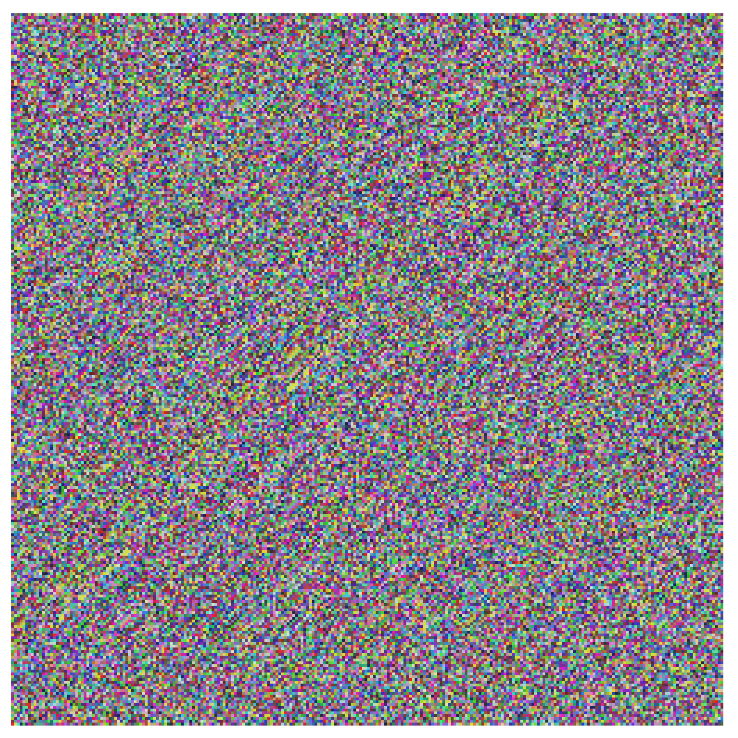In fact, this computational approach turns out to be an efficient way for dealing with Latin squares of much higher orders. To illustrate this fact, let us consider the Latin square of order 256 that is represented by colors in Figure 5. It was randomly constructed by following Algorithm 1 in [48], which gives rise to random Latin squares with possible implementation in cryptography. Notice in any case that every Latin square generated in this way is isotopic to a diagonally cyclic Latin square [49]. 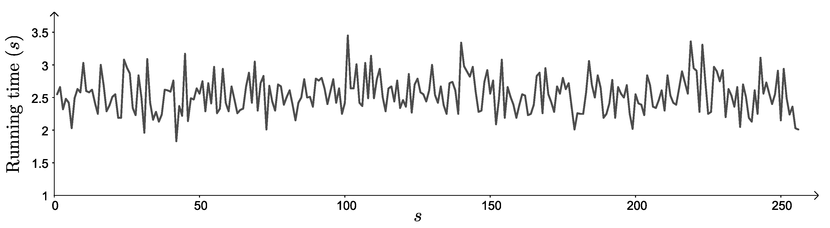Figure 6 shows the running time required by an Intel Core i7-8750H CPU (6 cores), with a 2.2 GHz processor and 8 GB of RAM for computing both the reduced Gröbner basis of the binomial ideal associated to the s-standard $90\times 90$ image pattern of this Latin square described in Figure 5, for every positive integer $s\le 256$, together with the cardinality of its related affine algebraic set. The maximum running time was $3.45$ s, which is reached for $s=101$.

It is remarkable that the methodology here described may be particularized in order to make more efficient the computation of group isomorphisms. Let us recall in this regard that every associative quasigroup constitutes a group. To illustrate this fact, let us consider both the dihedral and the abelian groups of order six, whose respective multiplication tables are the Latin squares

$${\mathcal{D}}_6\equiv \boxed{\begin{array}{cccccc}1& 2& 3& 4& 5& 6\\ 2& 3& 1& 5& 6& 4\\ 3& 1& 2& 6& 4& 5\\ 4& 6& 5& 1& 3& 2\\ 5& 4& 6& 2& 1& 3\\ 6& 5& 4& 3& 2& 1\end{array}}\mathrm{and}{\mathcal{Z}}_6\equiv \boxed{\begin{array}{cccccc}1& 2& 3& 4& 5& 6\\ 2& 3& 4& 5& 6& 1\\ 3& 4& 5& 6& 1& 2\\ 4& 5& 6& 1& 2& 3\\ 5& 6& 1& 2& 3& 4\\ 6& 1& 2& 3& 4& 5\end{array}}.$$

Their respective standard sets of $90\times 90$ image patterns are shown in the $2\times 6$ collage of Figure 7. Both standard sets are formed by a constant and five fractal standard image patterns. It is readily verified from a visual way that the standard set of the dihedral group (top row of the collage) does not coincide with the standard set of the abelian group (bottom row of the collage), even allowing a possible permutation of symbols. In this simple way, we may ensure that these two groups are not isomorphic.

A similar conclusion arises from the computation of the reduced Gröbner bases concerning both types of affine algebraic sets associated to the dihedral and the abelian group of order six. From this computation, we have that

$$|{\mathcal{V}}_{\mathbb{C}}\left(I\left({\mathcal{D}}_6\right)\right)|=3\mathrm{and}|{\mathcal{V}}_{\mathbb{C}}\left(I\left({\mathcal{Z}}_6\right)\right)|=7.$$

In addition, we have that $|{\mathcal{V}}_{\mathbb{C}}\left(I\left({\mathcal{P}}_{90,90;s}\left({\mathcal{D}}_6\right)\right)\right)|=\infty$, for every positive integer $s\le 6$, but

$$|{\mathcal{V}}_{\mathbb{C}}\left(I\left({\mathcal{P}}_{90,90;2}\left({\mathcal{Z}}_6\right)\right)\right)|=|{\mathcal{V}}_{\mathbb{C}}\left(I\left({\mathcal{P}}_{90,90;6}\left({\mathcal{Z}}_6\right)\right)\right)|=7.$$

Further, the methodology here described can be generalized for other types of arrays non-subjected to the Latin square condition. In this regard, it would be interesting to delve, for instance, into the study of standard sets of image patterns associated to (partial) semigroups or, more generally, to (partial) magmas. Even if they may not be endowed with a left or right division (as quasigroups are), their multiplication tables enable us to define $r\times m$ image patterns based on these algebraic structures by making use to this end of the corresponding conditions described in (2) (see [50], for a first approach in this regard in case of dealing with magmas).

These conditions may be taken into account to deal also with arrays related to other types of mathematical structures, not only algebraic ones. To illustrate this aspect, let us focus on the classical problem in graph theory of determining whether two given graphs are isomorphic or not. Every adjacency matrix of a given simple graph of order n is a binary symmetric $n\times n$ array with main diagonal of zeros. It may be considered the multiplication table of a finite magma of set of symbols $\{0,1,\dots ,n-1\}$ from which one could define $r\times m$ image patterns satisfying the corresponding conditions in (2). Then, standard sets of s-standard image patterns, with $s\in \{0,1\dots ,n-1\}$, could be defined similarly to those ones described in Section 3. In this way, the standard set of two isomorphic regular graphs would always coincide, up to permutations of symbols. This fact may therefore be used for distinguishing non-isomorphic regular graphs, even from a visual way. Thus, for instance, the following two arrays constitute respective incidence matrices of the complete graph $K_4$ and the cycle $C_4$.

$$\boxed{\begin{array}{cccc}0& 1& 1& 1\\ 1& 0& 1& 1\\ 1& 1& 0& 1\\ 1& 1& 1& 0\end{array}}\boxed{\begin{array}{cccc}0& 1& 0& 1\\ 1& 0& 1& 0\\ 0& 1& 0& 1\\ 1& 0& 1& 0\end{array}}$$

The standard sets of the $90\times 90$ image patterns associated to both graphs are shown in the $2\times 4$ collage of Figure 8. Notice that the standard set of the complete graph $K_4$ (top row of the collage) is formed by one constant and three fractal image patterns, whereas that one of the cycle $C_4$ is formed by one constant, two fractal and one almost constant (except for its first row, the 3-standard image pattern is monochromatic) image patterns. Hence, these two regular graphs are not isomorphic.

These examples illustrate the relevance that standard sets of image patterns may have for distributing distinct types of algebraic and combinatorial structures into isomorphism classes. A much more comprehensive study dealing with their recognition and analysis is required in any case. It is established as further work. Similar to the methodology here implemented, computational algebraic geometry may be an interesting approach to this end. Furthermore, notice that this paper has not dealt with the fractal gradation of the image patterns under consideration. A comprehensive analysis of their fractal dimensions is of particular interest in order to improve the efficiency of this computational approach.

This paper also focuses on the possible use of computational algebraic geometry for dealing with the distribution of partial Latin squares according to the equivalence relations of being either partial transpose or P-partial isotopic, for some subset $P\subset \left[n\right]\times \left[n\right]\times \left[n\right]$. An exhaustive enumeration of these classes is also established as further work. Concerning the distribution into P-partial isotopism classes, it is required to delve into the study of P-partial autotopisms (that is, P-partial isotopisms from a partial Latin square to itself) and make use of the Orbit-Stabilizer Theorem in a similar way to the already studied distribution of partial Latin squares into isotopism classes [18].

Again, the main limitation of the methodology here introduced is the high dependence on the number of variables required by each one of the affine algebraic sets under consideration. To see it, it has been made use of the already mentioned Algorithm 1 described in [48] in order to obtain random Latin squares on which the computational efficiency of using Gröbner bases has been checked for determining both the set of Latin squares that are partial transpose of another given Latin square, and the set of partial autotopisms of a Latin square. 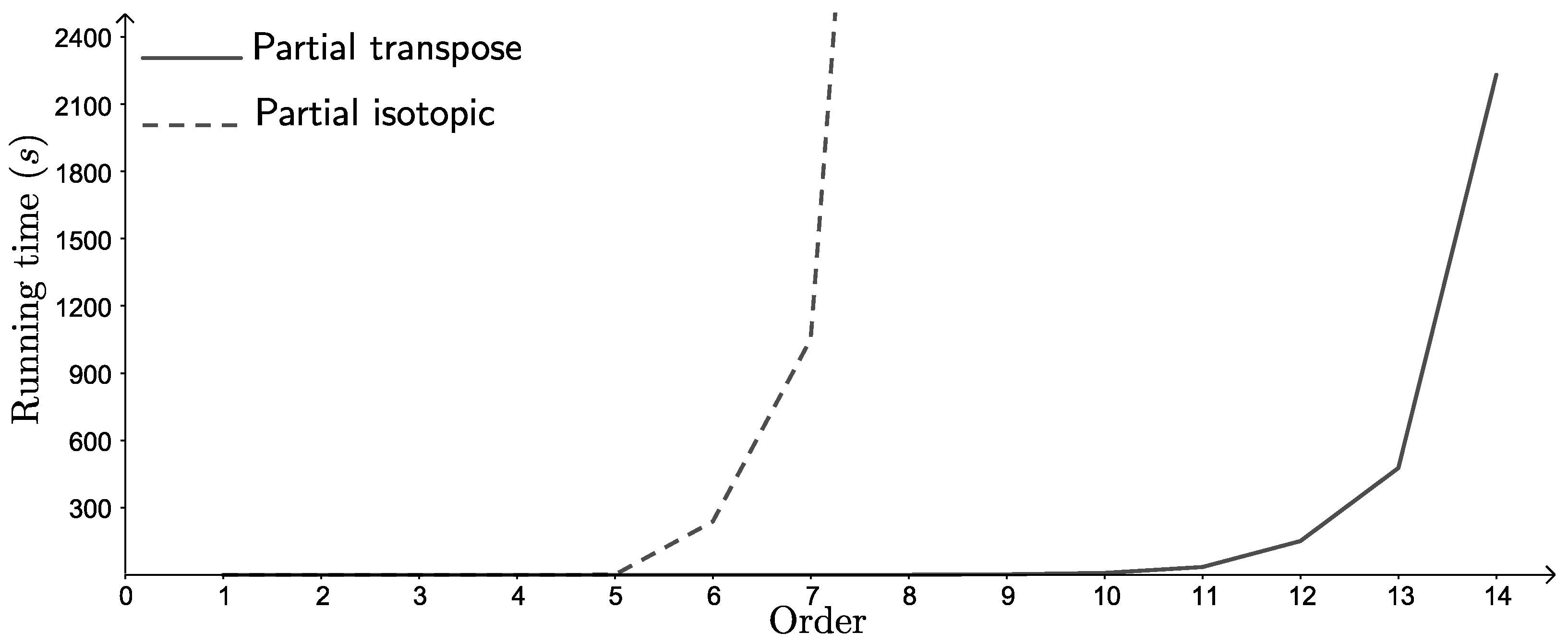Figure 9 shows the running time required by our computer system for computing both the reduced Gröbner basis of the corresponding ideal, together with the cardinality of its related affine algebraic set. Notice that only the relationship of being partial transpose seems to be useful for dealing by itself with the smallest orders for which no results on the distribution of Latin squares into isomorphism classes is known ($n\ge 12$). It is not the case of the equivalence relation of being P-partial isotopic, for some subset $P\subset \left[n\right]\times \left[n\right]\times \left[n\right]$, whose exponential growth starts visibly much before, even from order $n=5$. It agrees with the fact that this equivalence relation comprehends that one of being isotopic, for which previous studies [18] have already revealed the advantages of using some extra Latin square isomorphism invariant for reducing the computational cost of an analogous algebraic geometry approach. Similar studies concerning this new equivalence relation are, therefore, required and established as further work. In this regard, the joint use of the Latin square isomorphism invariants recently introduced in [34,35] may be of particular interest.

It is also interesting to illustrate the computational efficiency of these two approaches in case of dealing with partial Latin squares with empty cells, whose distribution into isomorphism classes is only known [17,18] for order $n\le 6$. Firstly, let us focus on the use of Gröbner bases for determining the set of partial Latin squares that are partial transpose of another given partial Latin square. To this end, a partial Latin square in the set ${\mathcal{L}}_{10;m}$ was randomly constructed, for each positive integer $m\le 100$, by means of Method (A) described in [34]. The latter consists of adding sequentially a set of feasible random entries to an empty partial Latin square until the desired weight is reached. 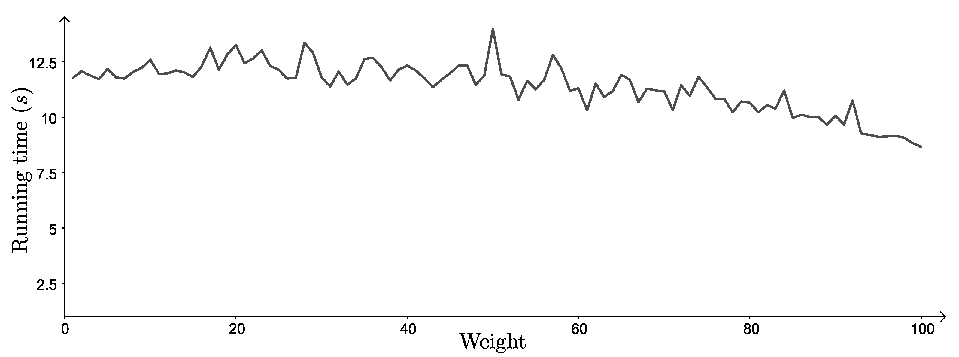Figure 10 shows the running time required by our computer system for determining both the reduced Gröbner basis of the corresponding ideals and the cardinalities of their related affine algebraic sets. The maximum running time was $13.99$ s, which is reached for $m=50$. It is remarkable the slightly decreasing tendency of this running time with respect to the weight of the partial Latin square under consideration.

Now, to illustrate the computational efficiency of using Gröbner bases for determining the set of P-partial isotopisms between two given partial Latin squares, for some subset $P\subset \left[n\right]\times \left[n\right]\times \left[n\right]$, the mentioned method of adding random entries has been used to construct a pair of random partial Latin squares in the set ${\mathcal{L}}_{7;m}$, for each positive integer $m\le 49$. 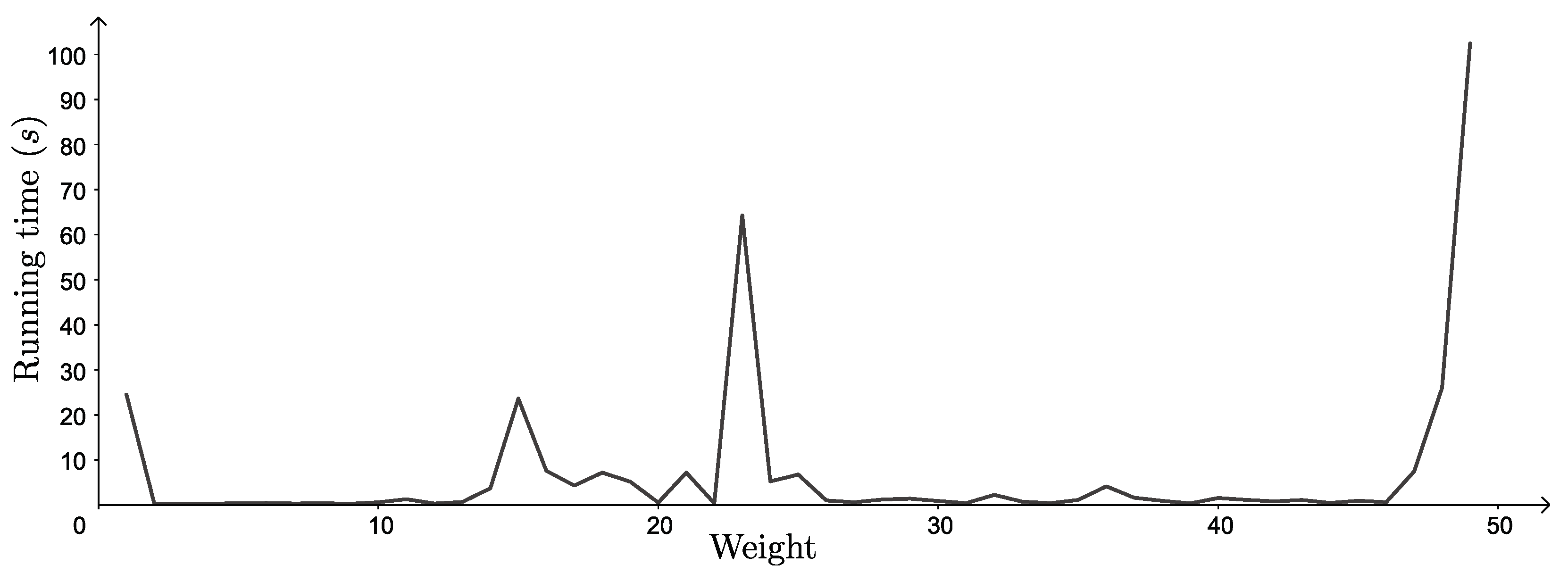(Recall that $n=7$ is the first order for which no result on the distribution into isotopism classes is known.) Figure 11 shows the running time required by our computer system for determining both the reduced Gröbner basis of the corresponding ideals and the cardinalities of their related affine algebraic sets. The maximum running time has been $102.43$ s, which is reached for $m=49$ (the Latin square case). The fast exponential growth of running time is remarkable for dense partial Latin squares. Partial Latin squares with either only one filled cell of with more or less the same number of empty and filled cells seem also to require more running time. All these cases turned out to be related to a high number of partial isotopisms. In any case, a much more comprehensive computational analysis concerning orders, weights and particular isomorphism classes of partial Latin squares is required for distinguishing potential bottlenecks in the computation of related Gröbner bases.

Let us finish this section by establishing the following open problems to deal also with as further work on this topic.

Problem 1.

What are the minimum and maximum numbers of partial Latin squares that are partial transpose of a partial Latin square in ${\mathcal{L}}_{n;m}$?

Problem 2.

What are the minimum and the maximum numbers of distinct partial Latin squares for which there is at least one P-partial isotopism to a partial Latin square in ${\mathcal{L}}_{n;m}$, for some subset $P\subset \left[n\right]\times \left[n\right]\times \left[n\right]$?

Problem 3.

What is the maximum cardinality of a subset $P\subset \left[n\right]\times \left[n\right]\times \left[n\right]$ for which a P-partial isotopism exists between two distinct partial Latin squares in ${\mathcal{L}}_{n;m}$?