
Calculation of Two Types of Quaternion Step Derivatives of Elementary Functions

Department of Mathematics, Dongguk University, Gyeongju 38066, Korea
Mathematics 2021, 9(6), 668; https://doi.org/10.3390/math9060668
Submission received: 20 February 2021
/
Revised: 14 March 2021
/
Accepted: 18 March 2021
/
Published: 21 March 2021
(This article belongs to the Special Issue Nonlinear Equations: Theory, Methods, and Applications)
Abstract
:We aim to get the step derivative of a complex function, as it derives the step derivative in the imaginary direction of a real function. Given that the step derivative of a complex function cannot be derived using i, which is used to derive the step derivative of a real function, we intend to derive the complex function using the base direction of the quaternion. Because many analytical studies on quaternions have been conducted, various examples can be presented using the expression of the elementary function of a quaternion. In a previous study, the base direction of the quaternion was regarded as the base separate from the basis of the complex number. However, considering the properties of the quaternion, we propose two types of step derivatives in this study. The step derivative is first defined in the j direction, which includes a quaternion. Furthermore, the step derivative in the direction is determined using the rule between bases i, j, and k defined in the quaternion. We present examples in which the definition of the j-step derivative and -step derivative are applied to elementary functions , , and .
MSC:
Primary 32G35; 32W50; 32A99; Secondary 11E881. Introduction
Sensitivity analysis is an important area in engineering research; hence, when selecting a sensitivity calculation method, the accuracy and computational cost must be considered. The commonly used method for sensitivity calculation is the finite difference. Although it lacks computational accuracy and efficiency, the biggest advantage of this method is that it is easy to implement. Analytical methods for sensitivity analysis are more accurate and can be classified in terms of the derivation and implementation. According to Martins et al. [1,2], the continuous approach for deriving the sensitivity equation of a given system involves the differentiation of the sensitivity equation followed by the discretization of the resulting sensitivity equation, before solving the numerical values. The alternative discrete approach involves the discretization of the governing equation followed by its differentiation to obtain a sensitivity equation that can be solved numerically.
The application of complex variables to develop estimates of the derivatives and Taylor’s formula have been extensively studied. Agarwal and Bohner [3] developed basic tools of calculus on time scales such as Taylor’s formula and L’Hôspital’s rule. Agarwal et al. [4] established inclusions involving the Riemann–Liouville fractional derivative. Lyness and Moler [5] and Lyness [6] introduced several methods using complex variables, including a reliable method for calculating the n-th derivative of an analytical function. This theory was used by Squire and Trapp [7] to obtain a simple expression for estimating the first derivative. The estimate, which was demonstrated as suitable for application in modern numerical calculations, can be easily implemented, while maintaining reasonable computational costs. Hence, this technique has been used for sensitivity analysis in a wide variety of environments, including computational fluid dynamics (see [8,9]). Lai and Crassidis [10,11] further examined the approach of Martins et al. [1,2], and based on the results of studying the derivation of the step derivative along the complex direction for a real function using the Taylor series expansion, a complex step differential approximation and its application to a numerical algorithm were presented (see [12,13,14,15]). Kim et al. [16,17,18] investigated the composition and properties of quaternion functions based on the algebraic features of quaternions. They suggested that the definitions of the function limit and the derivative are not uniquely determined by the noncommutativity of the product, which is a typical characteristic of the quaternary function basis. Therefore, by proposing various types of differential operators and applying differentiation calculations and results according to the shape of the differential operators, a theorem to replace the definition of the differential was presented.
Roelfs et al. [19] and Turner [15] defined the quaternion direction and proposed a step derivative of the complex function in the quaternion direction. They proposed the quaternion direction by using the properties of the complex-like form and the form corresponding to the Pauli matrix. In [15,19], although the quaternion number is a number system that extends the complex number, a step derivative was proposed by interpreting base i of the complex number as a separate base that can be exchanged without being treated as part of the quaternion-number base. Motivated by their approach, but unlike [15,19], this study focuses on the definition and structure of quaternions based on the original meaning proposed by Hamilton and proposes a step derivative by recognizing complex number i as the basis of the quaternion. This defines the step derivative of the complex function, while retaining the meaning and characteristics of the quaternion.
In this paper, we propose a definition of the quaternion step derivative for a complex function with reference to the method of deriving the complex step derivative for a real function. Considering the rule between the base of the quaternion and that of the complex number, we propose two types of step derivatives using the Taylor series expansion. In Section 1, the step derivative is first defined in the j direction, which includes a quaternion. As the derivative of the complex function should be included in the complex system, the step derivative is presented by specifying the terms included in the complex system in the Taylor series expansion using the property between i and j. Section 2 defines the step derivative in the direction. The step derivative in the direction is presented to apply the same magnitude and direction in the j and k directions using the rule between bases i, j, and k defined in the quaternion. In Section 1 and Section 2, we provide examples in which the definition of the j-step and -step derivatives are applied to elementary functions , , and . Further, the value of the step derivative at a certain point and the relative error of the derivative value determined using the differential method of the complex function are calculated. Based on the graphs for the calculated results, we demonstrate the effectiveness of the j-step and -step derivative values. In Section 3, the j-step derivative proposed in Section 1 and the -derivative proposed in Section 2 are compared, and the characteristics of each derivative depending on the direction of Taylor series expansion and the magnitude of h are summarized. In addition, as a future development plan, the step derivative of the quaternionic function is conceived of by defining the step derivative in the base direction of various Clifford algebras.
2. Quaternion -Step Derivative
Let be a set of quaternions denoted by:
satisfying , , , and . Now, considering the properties of the basis of the quaternion, we derive a new step derivative in the j-direction as follows:
A small step h is expanded in the direction of imaginary unit j of the quaternion, whose direction is different from that of imaginary unit i of the complex number. As per the definition of the Taylor series expansion,
where is a quaternion constant between z and , which means that it is located in a place not exceeding the real h size along the axis j perpendicular to the plane where the complex number z exists. If Equation (1) is rearranged to express the quaternionic step derivative of a complex-valued function of complex variable , we have:
The aim of this study is to determine how derivative of is obtained. Because the derivative of a complex function is defined in the complex system, we define . Let be a function that outputs only the complex numbers in ; i.e., from the quaternion applied to , the elements corresponding to the complex numbers are extracted. For example,
Hence,
We finally obtain the following equation:
The truncation about the derivative terms greater than or equal to two is motivated by referring to the error analysis in [2,10,11] containing the error analysis in the domain of the extension step from real functions to complex functions and in [15,19] containing the error analysis in the domain of the extension step from complex functions to quaternionic functions. Thus:
Definition 1.
For sufficiently small h, the first derivative of f can be derived using the following equation:
This is called the quaternion j-step derivative of f.
Using Definition 1, we find the quaternion j-step derivative for each following elementary function.
Example 1.
For a complex variable z, the quaternion j-step derivative of the exponential function can be calculated as follows:
and for sufficiently small ,
Let and be functions that print the actual and measured values, respectively. With the complex derivative, using the definition of complex analysis, we obtain . The for the function that will be used in the examples (we will cover later) is derived by [20]. For , the quaternion j-step derivative of is:
For , the relative error of the quaternion j-step derivative of is:
Figure 2 depicts the relative error of with respect to h.
Example 2.
As another example, for a complex variable z, the quaternion j-step derivative of the cosine function can be calculated as follows:
For sufficiently small ,
For , with the quaternion j-step derivative,
The relative error of the quaternion j-step derivative of at is:
where Figure 4 shows the relative error of with respect to h.
Example 3.
As another example, for a complex variable z, the quaternion j-step derivative of the sine function calculated as per the definition of the quaternion j-step derivative:
and for sufficiently small ,
For , with the quaternion j-step derivative,
As h approaches , the quaternion j-step derivative of at tends to the actual value by the definition of the derivative for a complex system. Furthermore, as h approaches , the relative error of at tends to zero. In particular, the relative error of the quaternion j-step derivative of at is equal to that of according to the calculation based on the definition of the quaternion j-step derivative. Therefore, Figure 4 also expresses the relative error of the quaternion j-step derivative of at .
3. Quaternion -Step Derivative
The basis of the quaternion is composed of . In the previous section, the step derivative was derived using j. We now derive the step derivative in the direction, including k as the basis of the quaternion, as follows:
As the direction of is distinct from that of i, which contains the complex-valued functions of a complex variable, we define a formula called the -step derivative using the Taylor series expansion for at z. With the Taylor series expansion, we have:
Multiplying both sides by ,
Applying to extract only the complex functions, we get:
Thus, we obtain the following formula:
Definition 2.
For a complex-valued function of a complex variable z, we have:
This is called the quaternion -step derivative of . As h approaches a sufficiently small value, the term tends to zero.
The quaternion -step derivative is derived with reference to the definition of the elementary functions of a quaternion variable summarized in [21]. Functions and are defined as follows:
and:
Referring to [21], we consider the quaternion -step derivative of the elementary functions.
Example 4.
For example, for a complex variable z, the quaternion -step derivative of the exponential function is as follows:
For , the quaternion -step derivative of is:
Figure 5 illustrates the quaternion -step derivative of at with respect to h.
For the true value of , the relative error of the quaternion -step derivative of at is:
which is depicted in Figure 6.
From Figure 6, we check how close the relative error of the quaternion -step derivative of approximated to zero for h values near is, compared to the j-step derivative.
Example 5.
For example, consider the quaternion -step derivative of cosine function . As per the definition of the quaternion -step derivative, the following equation is derived:
For , we obtain the quaternion -step derivative of at :
Figure 7 shows the quaternion -step derivative, the j-step derivative, and the typical definition of the complex derivative of at .
The relative error of the quaternion -step derivative of at is calculated as follows:
where:
which is shown in Figure 8.
Example 6.
For example, for a complex variable z, consider the sine function ; the quaternion -step derivative is as follows:
For , the value of the quaternion -step derivative of is:
4. Conclusions
The step derivative of a complex-valued function of a complex one-variable was defined based on the rules and properties of the quaternion basis. Using the quaternion system, the step derivative was defined by presenting a direction distinct from that of basis i of the complex function. The value of the derivative calculated as per the definition of the derivative in the complex system for an elementary complex function was compared with that defined as per the definition of the quaternion j-step derivative. Depending on the size of h, the quaternion j-step derivative was similar to the derivative value calculated as per the definition of the derivative used in the complex number system. The similarity was directly confirmed by calculating the relative error through examples of the elementary function. It was observed that as the size of h decreased or was near a specific value of h, the relative error of the derivative value at a certain point approached zero.
In addition, because the quaternion has j and k as the bases, the step derivative to which the quaternion characteristic was applied was investigated. A step derivative that can be applied simultaneously with j and k, the bases of the quaternion number, was defined. As both j and k are defined in different directions from i of the complex number, a step derivative that can be applied in the j and k directions simultaneously and with the same size was defined. The quaternion -step derivative has a relative error with the derivative value as per the limit definition of the complex function; however, the derivative value can be made similar by setting an appropriate h value.
As a future development plan, we will propose step derivatives in the base direction of various Clifford algebras for quaternion functions based on this study. It is expected that the problem caused by the noncommutativity of the product over the quaternion system will be solved and the derivative of a new perspective will be used. Indeed, given that the quaternion function has the noncommutative product for the basis, various forms of the definition of the Taylor series expansion exist for the quaternion function. As we derive the step derivative in the base direction of the quaternion for the complex function, we can derive the step derivative in the new base direction for the quaternion function. Hence, we can propose step derivatives in various directions in consideration of the properties of the quaternion function by using the algebraic properties and the results of the analytical definition of the quaternion. In particular, the limitations of the definition and use of limit operations and differential operators arising from the noncommutativity can be addressed. As the concept of difference can be derived from algebraic properties, the calculation can be expected to be easier. It is expected that a new perspective derivative can be used that is freed from the characteristic of the quaternion caused by the noncommutativity of the product.
Funding
This work was supported by the Dongguk University Research Fund 2019 and the National Research Foundation of Korea (NRF) (2017R1C1B5073944).
Institutional Review Board Statement
Not applicable.
Informed Consent Statement
Not applicable.
Conflicts of Interest
The author declare no conflict of interest.
References
- Martins, J.R.; Sturdza, P.; Alonso, J.J. The connection between the complex-step derivative approximation and algorithmic differentiation. In Proceedings of the 39th Aerospace Sciences Meeting and Exhibit, Reno, NV, USA, 8–11 January 2001. [Google Scholar]
- Martins, J.R.; Sturdza, P.; Alonso, J.J. The complex-step derivative approximation. ACM Trans. Math. Softw. 2003, 29, 142–149. [Google Scholar] [CrossRef] [Green Version]
- Agarwal, R.P.; Bohner, M. Basic calculus on time scales and some of its applications. Res. Math. 1999, 35, 3–22. [Google Scholar] [CrossRef]
- Agarwal, R.; Belmekki, M.; Benchohra, M. A survey on semilinear differential equations and inclusions involving Riemann-Liouville fractional derivative. Adv. Diff. Equ. 2009, 2009, 1–47. [Google Scholar] [CrossRef] [Green Version]
- Lyness, J.N.; Moler, C.B. Numerical differentiation of analytic functions. SIAM J. Numer. Anal. 1967, 4, 202–210. [Google Scholar] [CrossRef]
- Lyness, J.N. Numerical algorithms based on the theory of complex variable. In Proceedings of the ACM National Meeting (Washington, D.C.); ACM: New York, NY, USA, 1967; pp. 125–133. [Google Scholar]
- Squire, W.; Trapp, G. Using complex variables to estimate derivatives of real functions. SIAM Rev. 1998, 40, 110–112. [Google Scholar] [CrossRef] [Green Version]
- Newman, J.C.; Anderson, W.K.; Whitfield, L.D. Multidisciplinary Sensitivity Derivatives Using Complex Variables; Tech. Rep. MSSU-COE-ERC-98-08; Computational Fluid Dynamics Laboratory: Seoul, Korea, 1998. [Google Scholar]
- Newman, J.C., III; WhitZ̆field, D.L.; Anderson, W.K. Step-size independent approach for multidisciplinary sensitivity analysis. J. Aircr. 2003, 40, 566–573. [Google Scholar] [CrossRef]
- Lai, K.L.; Crassidis, J. Generalizations of the complex-step derivative approximation. In Proceedings of the AIAA Guidance, Navigation, and Control Conference and Exhibit, Keystone, CO, USA, 21–24 August 2006. [Google Scholar]
- Lai, K.L.; Crassidis, J.L. Extensions of the first and second complex-step derivative approximations. J. Comput. Appl. Math. 2008, 219, 142–149. [Google Scholar] [CrossRef] [Green Version]
- Cossette, C.C.; Walsh, A.; Forbes, J.R. The Complex-Step Derivative Approximation on Matrix Lie Groups. IEEE Robot. Autom. Lett. 2020, 5, 906–913. [Google Scholar] [CrossRef]
- Kumar, K. Expansion of a function of noncommuting operators. J. Math. Phys. 1965, 1965 6, 1923–1927. [Google Scholar] [CrossRef]
- Lantoine, G.; Russell, R.P.; Dargent, T. Using multicomplex variables for automatic computation of high-order derivatives. ACM Trans. Math. Softw. (TOMS) 2012, 38, 1–21. [Google Scholar] [CrossRef]
- Turner, J. Quaternion-based partial derivative and state transition matrix calculations for design optimization. In Proceedings of the 40th Aerospace Sciences Meeting and Exhibit, Reno, NV, USA, 14–17 January 2002. [Google Scholar]
- Kim, J.E.; Lim, S.J.; Shon, K.H. Regularity of functions on the reduced quaternion field in Clifford analysis. Abstr. Appl. Anal. 2014, 2014. [Google Scholar] [CrossRef] [Green Version]
- Kim, J.E.; Lim, S.J.; Shon, K.H. Taylor series of functions with values in dual quaternion. Pure Appl. Math. 2013, 20, 251–258. [Google Scholar] [CrossRef] [Green Version]
- Kim, J.E. The corresponding inverse of functions of multidual complex variables in Clifford analysis. J. Nonlinear Sci. Appl. 2016, 9, 4520–4528. [Google Scholar] [CrossRef] [Green Version]
- Roelfs, M.; Dudal, D.; Huybrechs, D. Quaternionic Step Derivative: Automatic Differentiation of Holomorphic Functions using Complex Quaternions. arXiv 2020, arXiv:2010.09543. [Google Scholar]
- Brown, J.W.; Churchill, R.V. Complex Variables and Applications, 8th ed.; McGraw-Hill Book Company: New York, NY, USA, 2009; Chapter 3. [Google Scholar]
- Georgiev, S.; Morais, J.; Spröss, W. New aspects on elementary functions in the context of quaternionic analysis. Cubo (Temuco) 2012, 14, 93–110. [Google Scholar] [CrossRef]
Figure 1.
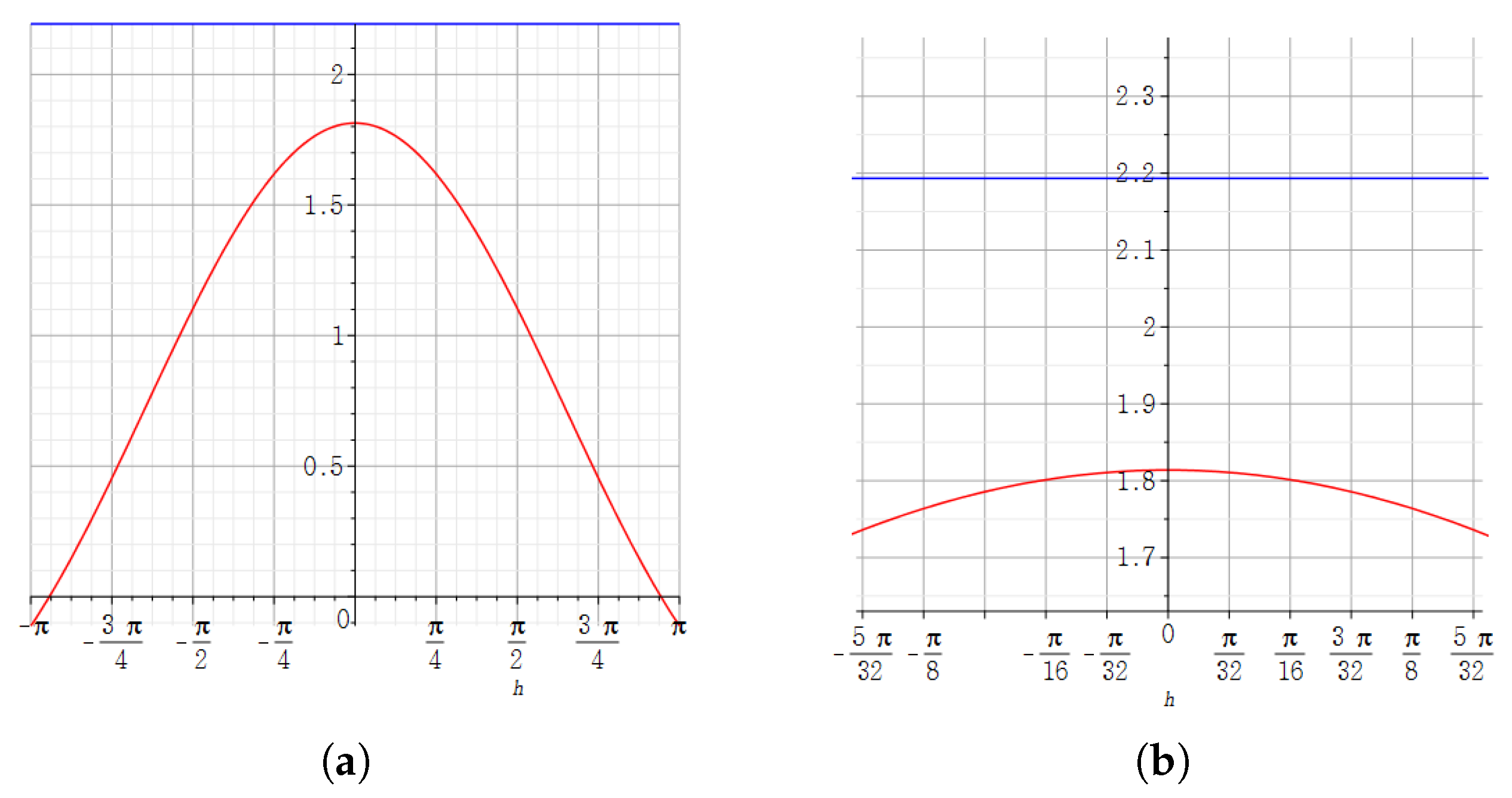
(a) The result obtained by using the Maple plot to see what the step derivative has according to the size of h. (b) In the graph of (a), the result of zooming in about h near zero. In (a,b), the red graph represents the j-step derivative of at according to the size of h, and the blue constant graph represents the absolute value of the derivative of at by the definition of the derivative for a complex system.
Figure 1.
(a) The result obtained by using the Maple plot to see what the step derivative has according to the size of h. (b) In the graph of (a), the result of zooming in about h near zero. In (a,b), the red graph represents the j-step derivative of at according to the size of h, and the blue constant graph represents the absolute value of the derivative of at by the definition of the derivative for a complex system.

Figure 2.
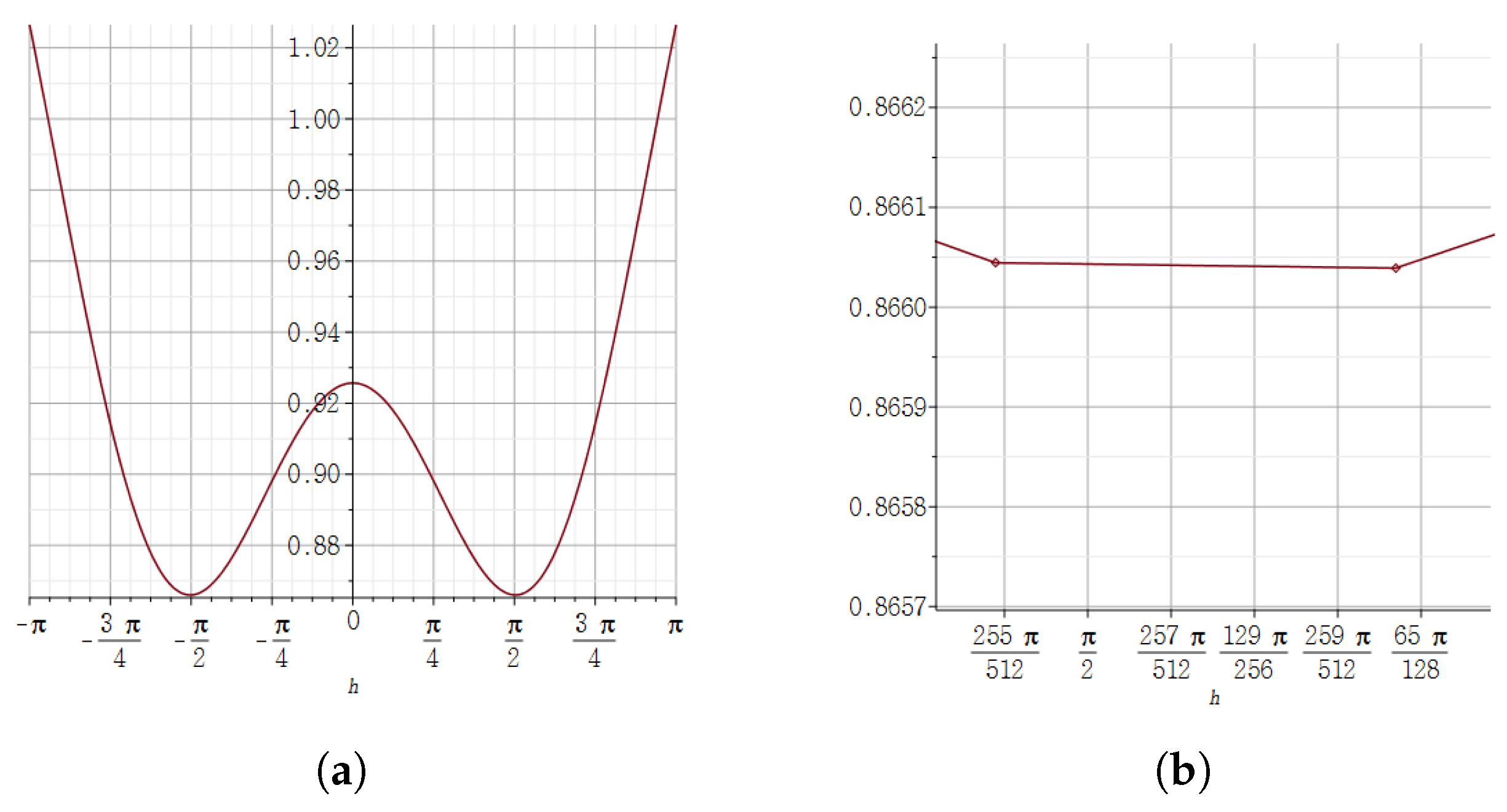
(a) The result of expressing the value of the relative error of the quaternion j-step derivative of at on the vertical axis according to the size of the horizontal axis h using the Maple plot. (b) In the graph of (a), the result of zooming in about h near . It confirms to us how close the relative error is to zero.
Figure 2.
(a) The result of expressing the value of the relative error of the quaternion j-step derivative of at on the vertical axis according to the size of the horizontal axis h using the Maple plot. (b) In the graph of (a), the result of zooming in about h near . It confirms to us how close the relative error is to zero.

Figure 3.
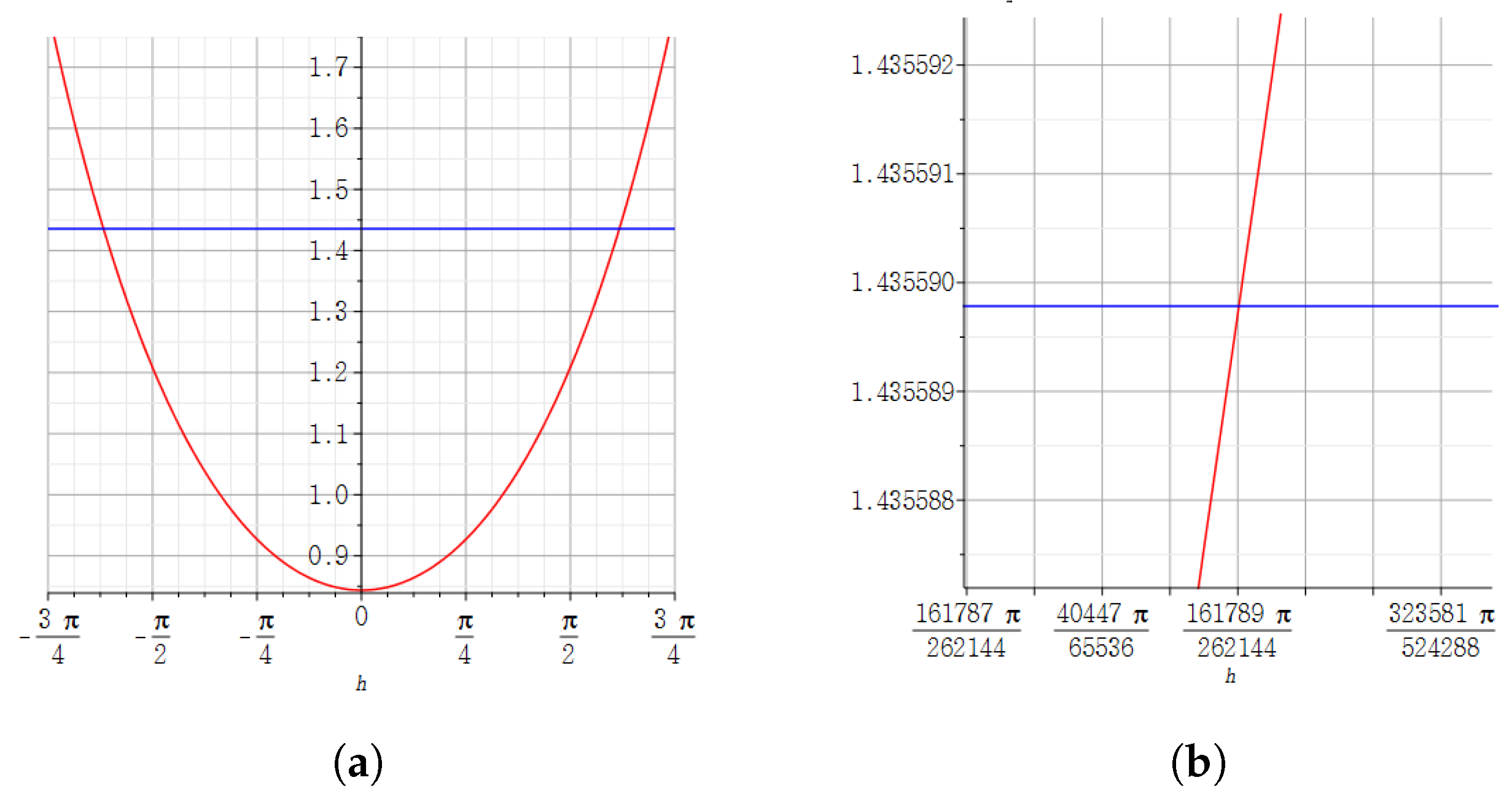
(a) Graph showing the absolute value of the quaternion j-step derivative of at according to the step size h driven by the Maple program. (b) In the graph of (a), the result of zooming in about h near . In (a,b), the red graph represents the j-step derivative of at according to the size of h, and the blue constant graph represents the absolute value of the derivative of at by the definition of the derivative for a complex system.
Figure 3.
(a) Graph showing the absolute value of the quaternion j-step derivative of at according to the step size h driven by the Maple program. (b) In the graph of (a), the result of zooming in about h near . In (a,b), the red graph represents the j-step derivative of at according to the size of h, and the blue constant graph represents the absolute value of the derivative of at by the definition of the derivative for a complex system.

Figure 4.
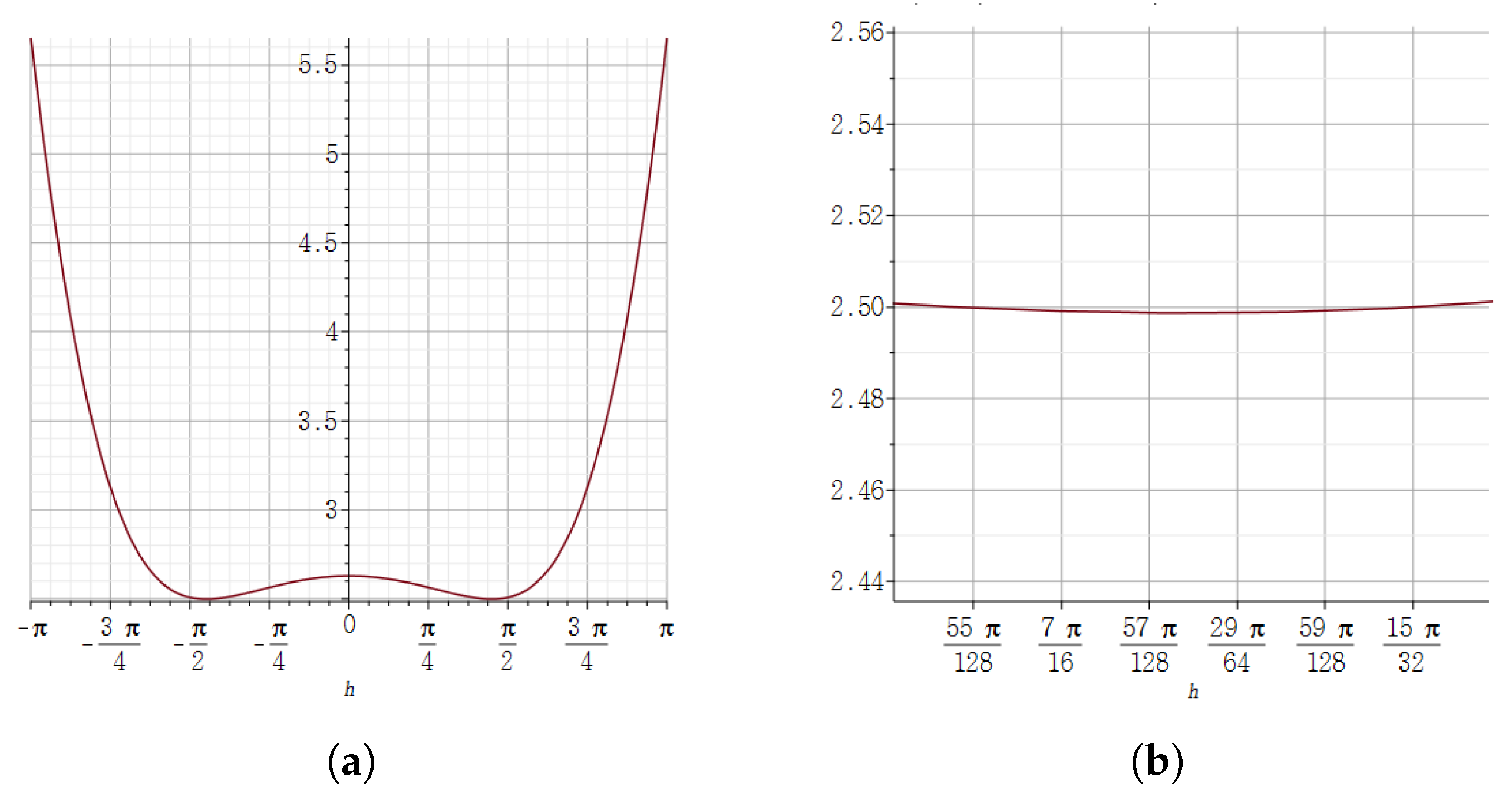
(a) The result of expressing the value of the relative error of the quaternion j-step derivative of at on the vertical axis according to the size of the horizontal axis h using the Maple plot. (b) In the graph of (a), the result of zooming in about h near . It confirms to us how close the relative error is to zero.
Figure 4.
(a) The result of expressing the value of the relative error of the quaternion j-step derivative of at on the vertical axis according to the size of the horizontal axis h using the Maple plot. (b) In the graph of (a), the result of zooming in about h near . It confirms to us how close the relative error is to zero.

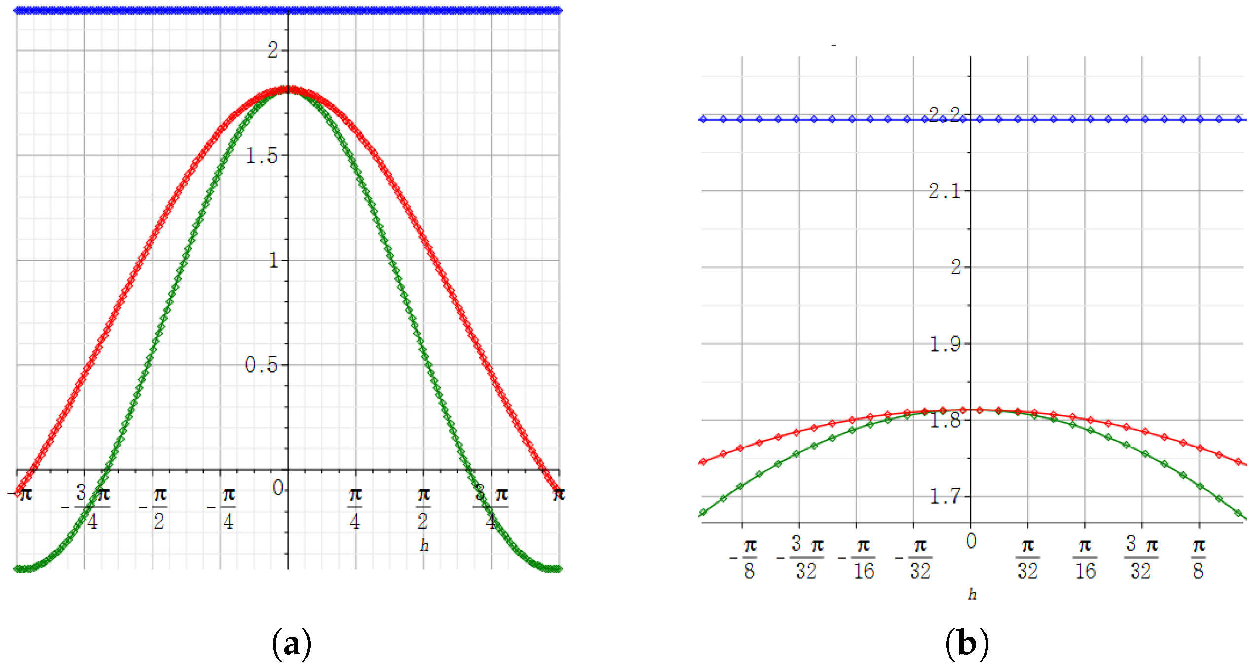
Figure 5.
(a) The result obtained by using the Maple plot to see what the step derivative has according to the size of h. (b) In the graph of (a), the result of zooming in about h near zero. In (a,b), according to the size of h, the green graph represents the -step derivative, the red graph represents the j-step derivative of at , and the blue constant graph represents the absolute value of the derivative of at by the definition of the derivative for a complex system.

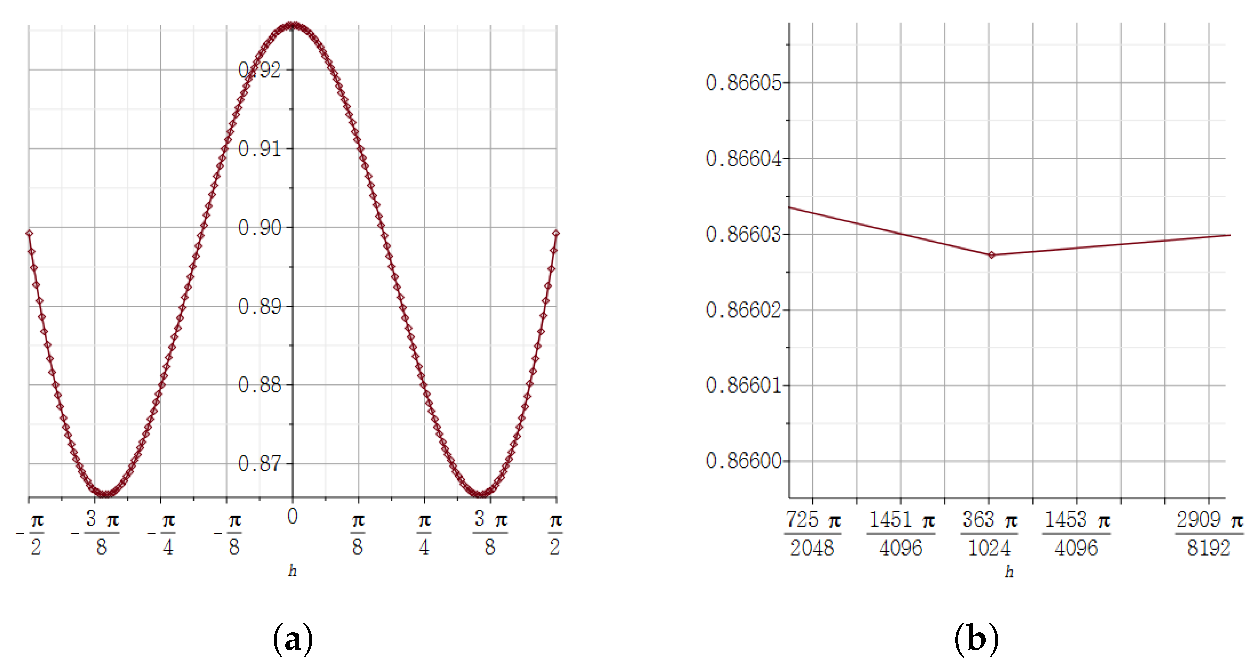
Figure 6.
(a) The result of expressing the value of the relative error of the quaternion -step derivative of at on the vertical axis according to the size of the horizontal axis h using the Maple plot. (b) In the graph of (a), the result of zooming in about h near . It confirms to us how close the relative error is to zero.

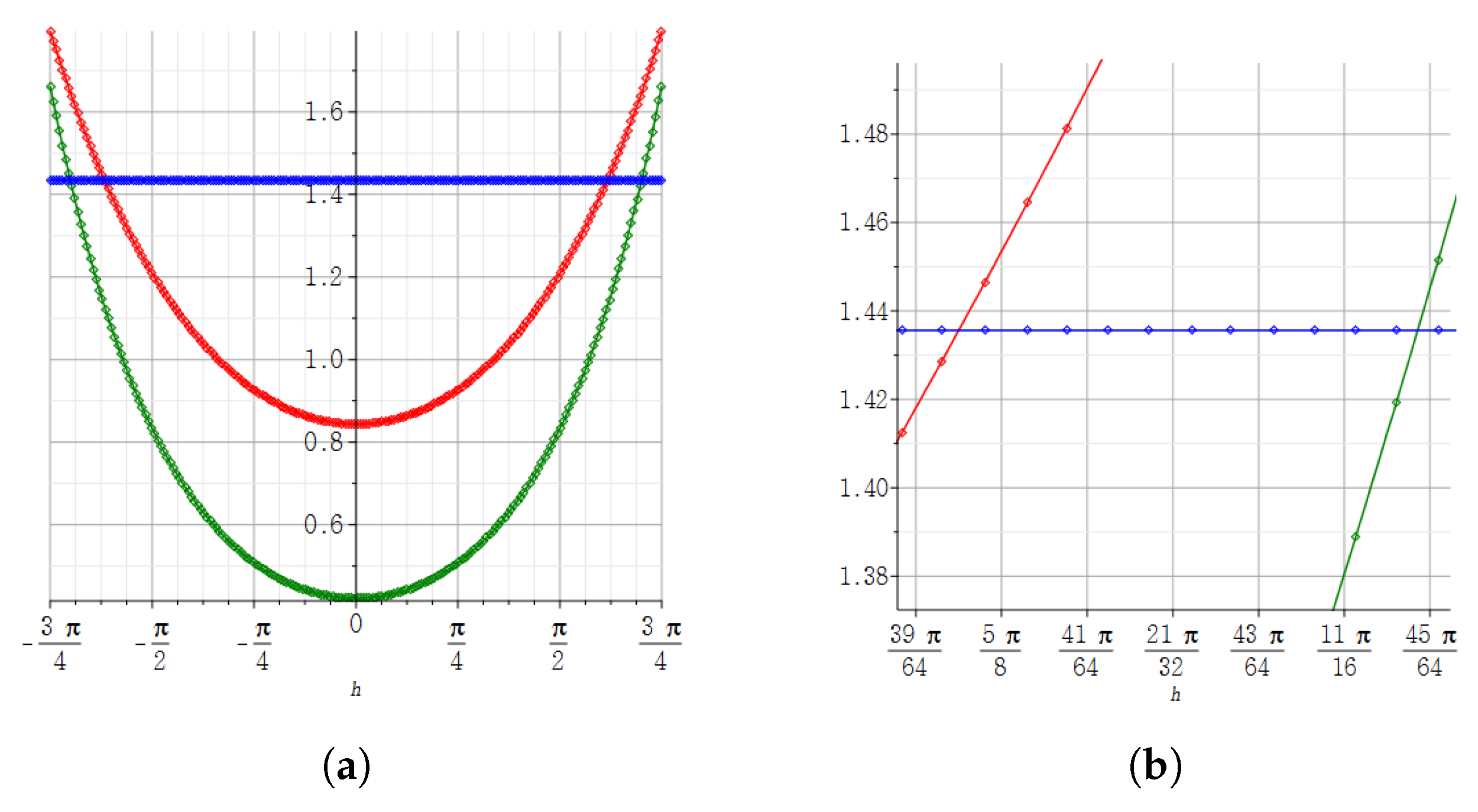
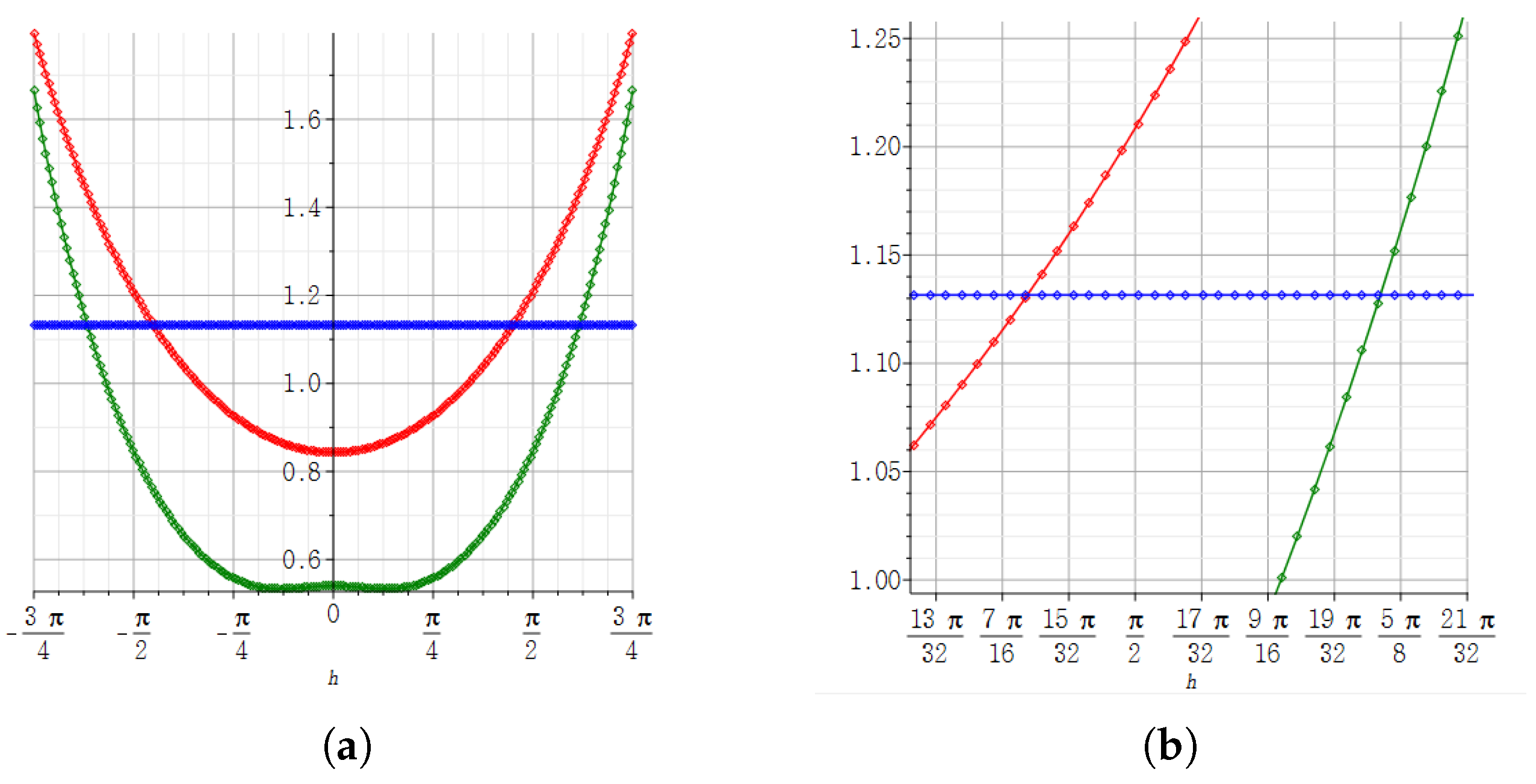
Figure 7.
(a) The result obtained by using the Maple plot to see what the step derivative has according to the size of h. (b) In the graph of (a), the result of zooming in about h near the midpoints of and . In (a,b), the green graph represents the -step derivative, the red graph represents the j-step derivative of at according to the size of h, and the blue constant graph represents the absolute value of the derivative of at by the definition of the derivative for a complex system.

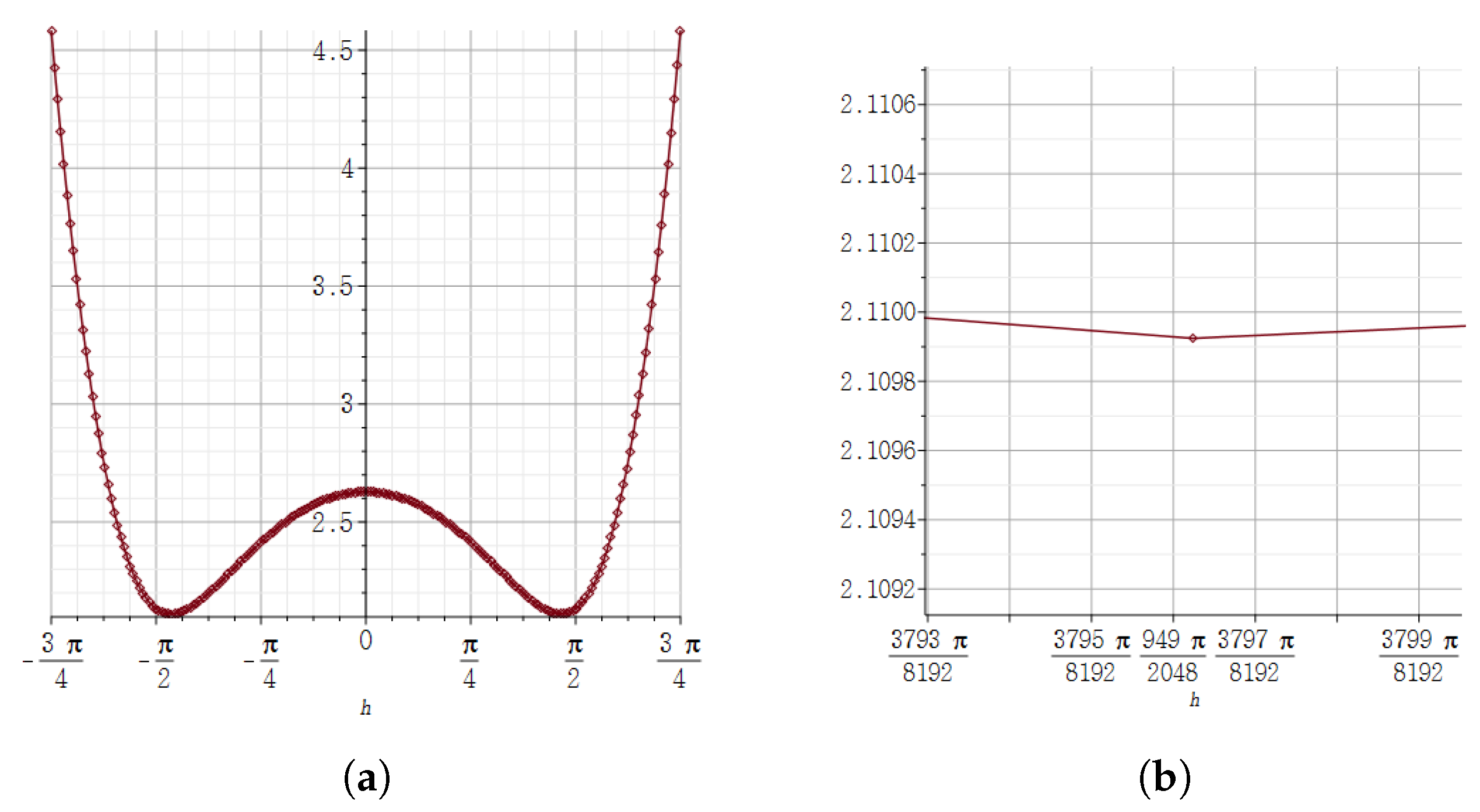
Figure 8.
(a) The result of expressing the value of the relative error of the quaternion -step derivative of at on the vertical axis according to the size of the horizontal axis h using the Maple plot. (b) In the graph of (a), the result of zooming in about h near . The quaternion -step derivative of has a relative error approximated to zero for h near .

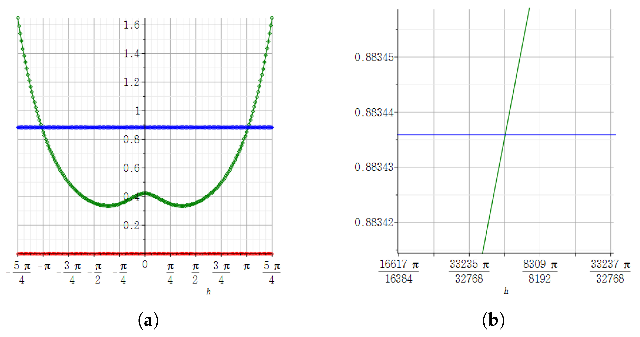
Figure 9.
(a) shows the result of the real part of the step derivatives of at according to the size of h by using the Maple plot. (b) In the graph of (a), the result of zooming in about h near the midpoints of and . In (a,b), the green graph represents the real part of the -step derivative, the red graph represents the real part of the j-step derivative of at according to the size of h, and the blue constant graph represents the real part of the derivative of at by the definition of the derivative for a complex system.

Figure 10.
(a) shows the result of the imaginary part of the step derivatives of at according to the size of h by using the Maple plot. (b) In the graph of (a), the result of zooming in about h near . In (a,b), the green graph represents the imaginary part of the -step derivative, the red graph represents the imaginary part of the j-step derivative of at according to the size of h, and the blue constant graph represents the imaginary part of the derivative of at by the definition of the derivative for a complex system.

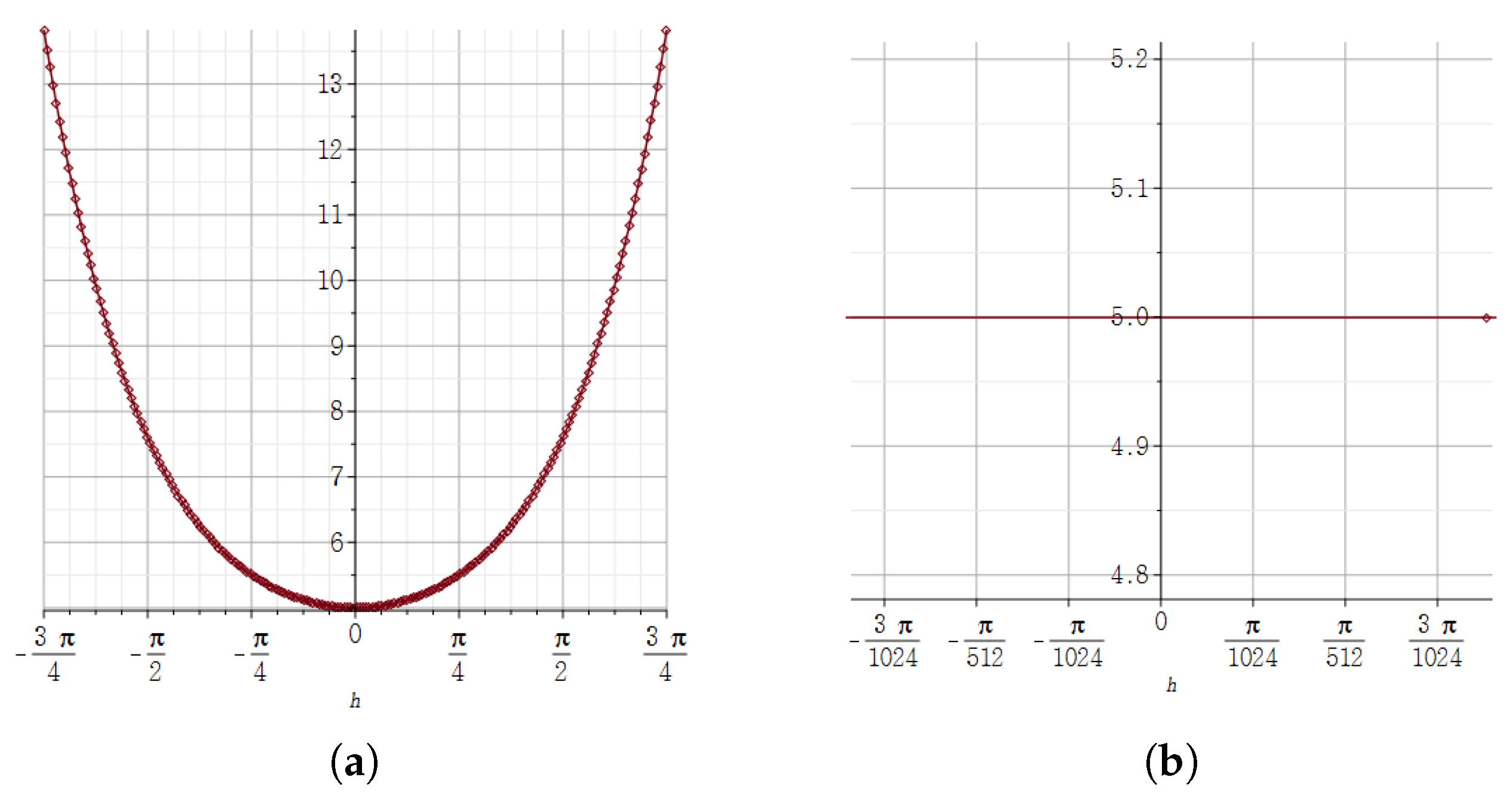
Figure 11.
(a) The result of expressing the value of the relative error of the quaternion -step derivative of at on the vertical axis according to the size of the horizontal axis h using the Maple plot. (b) In the graph of (a), the result of zooming in about h near zero. It confirms that the quaternion -step derivative of has a relative error approximated to the minimum value for h near zero.

Publisher’s Note: MDPI stays neutral with regard to jurisdictional claims in published maps and institutional affiliations. |
© 2021 by the author. Licensee MDPI, Basel, Switzerland. This article is an open access article distributed under the terms and conditions of the Creative Commons Attribution (CC BY) license (http://creativecommons.org/licenses/by/4.0/).
Share and Cite
MDPI and ACS Style
Kim, J.E. Calculation of Two Types of Quaternion Step Derivatives of Elementary Functions. Mathematics 2021, 9, 668. https://doi.org/10.3390/math9060668
AMA Style
Kim JE. Calculation of Two Types of Quaternion Step Derivatives of Elementary Functions. Mathematics. 2021; 9(6):668. https://doi.org/10.3390/math9060668
Chicago/Turabian StyleKim, Ji Eun. 2021. "Calculation of Two Types of Quaternion Step Derivatives of Elementary Functions" Mathematics 9, no. 6: 668. https://doi.org/10.3390/math9060668
Note that from the first issue of 2016, this journal uses article numbers instead of page numbers. See further details here.