Computational Analysis and Bifurcation of Regular and Chaotic Ca²⁺ Oscillations

Abstract

This study investigated the stability and bifurcation of a nonlinear system model developed by Marhl et al. based on the total Ca²⁺ concentration among three different Ca²⁺ stores. In this study, qualitative theories of center manifold and bifurcation were used to analyze the stability of equilibria. The bifurcation parameter drove the system to undergo two supercritical bifurcations. It was hypothesized that the appearance and disappearance of Ca²⁺ oscillations are driven by them. At the same time, saddle-node bifurcation and torus bifurcation were also found in the process of exploring bifurcation. Finally, numerical simulation was carried out to determine the validity of the proposed approach by drawing bifurcation diagrams, time series, phase portraits, etc.

1. Introduction

Ca²⁺ is one of the vital ions for information processing in humans. It generally acts as a biological messenger in different cell types and is an indispensable ion for various physiological activities in the human body [1,2,3,4]. Ca²⁺ plays a particularly important role in the regulation and control of body functions. It is involved in the mechanism of heartbeat and thrombin formation, but also transmits neural signaling, modifies the enzyme activity, and regulates the mechanisms underlying the maturation and fertilization of germ cells. A phenomenon observed experimentally in most cell types is that intracellular Ca²⁺ concentration remains stable without stimulation. Some Ca²⁺ enter the cytosol from the Ca²⁺ store when the cell is stimulated, leading to an increment in Ca²⁺ concentration that triggers a series of physiological activities [5,6,7,8,9,10,11,12,13]. The cell adjusts itself and closes the Ca²⁺ channels when the stimulation increases to a certain extent, and then Ca²⁺ is taken up by Ca²⁺ stores. After a while, the intracellular Ca²⁺ concentration gains stability, and the cell returns to a resting state. The source of intracellular Ca²⁺ is mainly through the influx of extracellular Ca²⁺ and the release of Ca²⁺ stored in the endoplasmic reticulum or sarcoplasmic reticulum. The latter is mainly based on the mechanism of Ca²⁺ release from intracellular Ca²⁺ stores triggered by Ca²⁺ signaling, namely Ca²⁺-induced Ca²⁺ release [14,15,16].

Over the past few years, many investigations have been carried out on evoked Ca²⁺ dynamics. Oscillations of free Ca²⁺ concentrations are highly significant and ubiquitous control mechanisms in a large number of cells. Experimental evidence has demonstrated that Ca²⁺ oscillations have different characteristics such as regularity and chaos. Chaos refers to dynamic systems that are sensitive to initial values, resulting in unpredictable random motion. Chaotic motion has been associated with making long-term weather predictions and the discovery of Lorentz attractors. In physiology, various arrhythmias, atrioventricular block, and ventricular fibrillation may also be associated with chaos. A well-known manifestation of chaos is the butterfly effect. This refers to a small change that brings about widely varying consequences for the future as it continues to pass and has long been applied to the weather and the stock market. In psychology, for example, when a person receives a small psychological stimulus in childhood, as they grow older, this stimulus can have a large impact on them in adulthood. In addition, the approach to chaos mainly consists of period doubling bifurcations, quasi-periodic transitions, and intermittent chaos. The period doubling bifurcation can be seen in the bifurcation diagram.

After the discovery of oscillations by Wood et al. [17,18], Ca²⁺ oscillations have been extensively studied. Ca²⁺ oscillations can be classified into two types: the first type is simple Ca²⁺ oscillations, and the second is bursting. Simple Ca²⁺ oscillations have been explored extensively. In the experiments of Borghans et al. (1997), some more complex forms of Ca²⁺ oscillations have been found such as bursts and chaos. When the system enters chaos, the Ca²⁺ oscillations show an extremely sensitive dependence on the initial value. Borghans et al. and Houart et al. further proposed several possible mechanisms to explain the complex intracellular Ca²⁺ oscillations and performed mathematical analysis [19,20]. Chay also proposed a model for Ca²⁺ oscillations in excitable cells [21], and Shen and Larter (1995) studied complex Ca²⁺ oscillations and chaotic phenomena in non-excitable cells [22,23]. In these models, it is almost certain that the burst results from changes in IP₃ yields because IP₃ can stimulate Ca²⁺ channels and release a large number of Ca²⁺ into the cytosol or take up Ca²⁺ from the cytosol, thereby participating in Ca²⁺ regulation. This is one of the most straightforward explanations for the bursting of intracellular Ca²⁺. One mechanism proposed by Borghans et al. to explain complex Ca²⁺ oscillations is that bursting oscillations are associated with Ca²⁺-releasing channel activities in the endoplasmic reticulum. A further mechanism investigated in the same study is that there is not just one intracellular Ca²⁺ store. Both IP₃-sensitive and non-sensitive Ca²⁺ stores have been taken into account. In all models, the endoplasmic reticulum is the primary Ca²⁺ store for intracellular Ca²⁺.

Marhl et al. suggested the significance of free Ca²⁺ concentrations in mitochondria for Ca²⁺ oscillations and proposed a likely explanation for Ca²⁺ oscillations in cells [24]. In this study, the model focuses on Ca²⁺ exchange in the middle of the cytosol, endoplasmic reticulum, and mitochondria. The Ca²⁺ considered in the model includes cytosol, endoplasmic reticulum, and mitochondrial Ca²⁺ [25,26] and binds Ca²⁺ in the cytosol. These models well simulate enriched Ca²⁺ oscillations in cells. Nevertheless, in past investigations, the changes induced by different values of Ca_tot have not been discussed in detail. Moreover, most of the literature has focused on experiments, rarely analyzing the principles of Ca²⁺ oscillations theoretically. Therefore, this study takes Marhl et al.’s Ca²⁺ oscillation model as the research object, selects Ca_tot as a bifurcation parameter, analyzes the features of equilibrium by the qualitative theory of differential equation, and discusses the bifurcation of equilibrium by the bifurcation and center manifold theory [27,28,29,30]. The qualitative theory of differential equations allows for analysis of the characteristics of the equilibrium point of the system including stability, coordinates, and types. Specifically, the analysis was conducted using eigenvalues and the Hurwitz criterion. In addition, when investigating the bifurcation of higher-order nonlinear dynamic systems, the center manifold theory can transform the study of various behaviors of n-dimensional dynamic systems approaching equilibrium into the study of equations on m-dimensional (m < n) center manifolds, simplifying the system. Finally, the model was simulated numerically using AUTO and MATLAB in this study. The advantage is that it confirms our conclusions [31,32].

2. Description of the Model

The model established by Marhl et al. investigated the oscillation of free Ca²⁺ concentrations in the cytosol, endoplasmic reticulum, and mitochondria. A mathematical model was established to simulate the oscillation of intracellular Ca²⁺ concentration, and the specific system is as follows [24]:

$$\left\{\begin{array}{l}\frac{dC{a}_{cyt}}{dt}=J_{ch}+J_{leak}+J_{out}-J_{pump}-J_{in}+k_{-}CaPr-k_{+}C{a}_{cyt}Pr\\ \frac{dC{a}_{er}}{dt}=\frac{{\beta }_{er}}{{\rho }_{er}}(J_{pump}-J_{ch}-J_{leak})\\ \frac{dC{a}_m}{dt}=\frac{{\beta }_m}{{\rho }_m}(J_{in}-J_{out})\end{array}\right.,$$

(1)

where Ca_cyt is the cytosolic Ca²⁺ concentration; Ca_er is the Ca²⁺ concentration in the endoplasmic reticulum; Ca_m is the Ca²⁺ concentration in mitochondria; and Ca_tot is the conservation of total extracellular Ca²⁺. Details of the specific meaning and value of each parameter can be referred to in

Table 1. Unless otherwise specified, the parameter values are used as given in this model.

Prtot	120 μM	kpump	20 s−1
ρer	0.01	kout	125 s−1
ρm	0.01	km	0.00625 s−1
βer	0.0025	k−	0.01 s−1
βm	0.0025	K1	5 μM
kch	1500 s−1	K2	0.8 μM
kleak	0.05 s−1	K3	5 μM
kin	300 μM−1 s−1	k+	0.1 μM−1 s−1

and [24]. These parameters have the following relationships:

$$\begin{array}{l}{J}_{pump}=k_{pump}C{a}_{cyt}, P{r}_{tot}=Pr+CaPr, J_{out}=(k_{out} \frac{C{a}_{{cyt}^2}}{K_3^2+C{a}_{{cyt}^2}}+k_m )C{a}_m, J_{in}=k_{in} \frac{C{a}_{{cyt}^8}}{K_2^8+C{a}_{{cyt}^8}},\\ J_{ch}=k_{ch} \frac{C{a}_{cyt}{}^2}{K_1^2+C{a}_{cyt}{}^2} \left(C{a}_{er}-C{a}_{cyt}\right), CaPr=C{a}_{tot}-C{a}_{cyt}-\frac{{\rho }_{er}}{{\beta }_{er}}C{a}_{er}-\frac{{\rho }_m}{{\beta }_m}C{a}_m,\\ J_{leak}=k_{leak}\left(C{a}_{er}-C{a}_{cyt}\right).\end{array}$$

3. Results

3.1. Analysis of Stability

Ca_tot corresponds to the total intracellular Ca²⁺ concentration including free Ca²⁺ in the cytosol, endoplasmic reticulum, and mitochondria. The model ignores the exchange between extracellular and cytosolic Ca²⁺ and focuses on the regulation of Ca²⁺ concentration in the cytosol and organelles. In cells, Ca²⁺ generally exists in the organelles as free or protein-bound. Ca²⁺ can be induced to increase or decrease either by binding to buffer proteins or by the dissociation of binding Ca²⁺.

There are two principal ways in which Ca²⁺ is regulated: absorption and liberation of Ca²⁺ by the endoplasmic reticulum and mitochondria. Therefore, during the process, a series of experimental manipulations can be carried out to change the Ca²⁺ concentration in organelles. Then, Ca_tot will be changed in value. For example, intracellular injection of IP₃ leads to the liberation of Ca²⁺ in the endoplasmic reticulum, or Ca²⁺ pump inhibitors are used to inhibit Ca²⁺ uptake from the endoplasmic reticulum, thereby increasing free cytosolic Ca²⁺. Based on the above reasons, Ca_tot is a reasonable selection as the parameter that can be changed in the experiment. This is a practical guide for the experiment. Therefore, Ca_tot was chosen as the bifurcation parameter to discuss the existence, quantity, type, and bifurcation of the equilibrium.

To make the calculations easier, we can make x = Ca_cyt, y = Ca_er, z = Ca_m, r = Ca_tot. Therefore, model (1) can be transformed into the following expression:

$$\left\{\begin{array}{ll}\frac{dx}{dt}=& 0.01r+0.01y-20.06x-0.04z-0.1x(x-r+4y+4z+120)\\ & -\frac{1500x^2(x-y)}{x^2+25}-\frac{300x^8}{x^8+0.16777216}+z(\frac{125x^2}{x^2+25}+0.00625)\\ \frac{dy}{dt}=& 5.0125x-0.0125y+\frac{375x^2(x-y)}{x^2+25}\\ \frac{dz}{dt}=& -0.25z(\frac{125x^2}{x^2+25}+0.00625)+\frac{75x^8}{x^8+0.16777216}\end{array}\right..$$

(2)

One can immediately see that the equilibrium point of system (2) meets the following equation:

$$\left\{\begin{array}{l}0.01r-20.06x+0.01y-0.04z-0.1x(x-r+4y+4z+120)-\frac{1500x^2(x-y)}{x^2+25}\\ -\frac{300x^8}{x^8+0.16777216}+z(\frac{125x^2}{x^2+25}+0.00625)=0\\ 5.0125x-0.0125y+\frac{375x^2(x-y)}{x^2+25}=0\\ -0.25z(\frac{125x^2}{x^2+25}+0.00625)+\frac{75x^8}{x^8+0.16777216}=0\end{array}\right.$$

(3)

First, by calculating

$$-0.25z(\frac{125x^2}{x^2+25}+0.00625)+\frac{75x^8}{x^8+0.16777216}=0,$$

we can obtain

$$z=\frac{75x^8}{(\frac{31.25x^2}{x^2+25}+0.0015625)(x^8+0.167772)}.$$

Then,

$$5.0125x-0.0125y+\frac{375x^2(x-y)}{x^2+25}=0$$

can be calculated to obtain

$$y=\frac{30401x^3+10025x}{30001x^2+25}.$$

Consequently, substituting the expression for y and z obtains

$$\begin{array}{l}0.01r-20.06x+0.01y-0.04z-0.1x(x-r+4y+4z+120)-\frac{1500x^2(x-y)}{x^2+25}\\ -\frac{300x^8}{x^8+0.16777216}+z(\frac{125x^2}{x^2+25}+0.00625)=0.\end{array}$$

Therefore, we have the following equation:

$$\left\{\begin{array}{l}f(x,r)=0.01r-20.06x-0.1x(x-r+\frac{4{\sigma }_2}{{\sigma }_3}+\frac{300x^8}{{\sigma }_1}+120)-\frac{3x^8}{{\sigma }_1}+\frac{0.01{\sigma }_2}{{\sigma }_3}\\ -\frac{300x^8}{x^8+0.16777216}-\frac{1500x^2(x-\frac{{\sigma }_2}{{\sigma }_3})}{x^2+25}+\frac{75x^8(\frac{125x^2}{x^2+25}+0.00625)}{{\sigma }_1}=0\\ y=\frac{30401x^3+10025x}{30001x^2+25}\\ z=\frac{75x^8}{{\sigma }_1}\end{array}\right.,$$

(4)

where

$${\sigma }_1=(\frac{31.25x^2}{x^2+25}+0.0015625)(x^8+0.167772), {\sigma }_2=30401x^3+10025x, {\sigma }_3=30001x^2+25.$$

Depending on the practical implications of x, y, z, and r, whether Equation (2) has an equilibrium point was considered to meet our special needs when r $\in$ [0, 150]. Suppose (x₀, y₀, z₀) is equilibrium. Let x₁ = x − x₀, y₁ = y − y₀, z₁ = z − z₀, then we can obtain the following representations [30]:

$$\left\{\begin{array}{ll}\frac{d{x}_1}{dt}=& 0.01r-20.06\left(x_1+x_0\right)+0.01\left(y_1+y_0\right)-0.04\left(z_1+z_0\right)-0.1\left(x_1+x_0\right)(4(y_1\\ & +y_0)+4\left(z_1+z_0\right)+120+x_1+x_0-r)-\frac{1500{(x_1+x_0)}^2\left(x_1+x_0-y_1-y_0\right)}{{(x_1+x_0)}^2+25}\\ & -\frac{300{(x_1+x_0)}^8}{{(x_1+x_0)}^8+0.16777216}+z\left(\frac{125{(x_1+x_0)}^2+0.00625(\left(x_1+x_0{)}^2+25\right)}{{(x_1+x_0)}^2+25}\right)\\ \frac{d{y}_1}{dt}=& -0.0125\left(y_1+y_0\right)+5.0125\left(x_1+x_0\right)+\frac{375{(x_1+x_0)}^2\left(x_1+x_0-y_1-y_0\right)}{{(x_1+x_0)}^2+25}\\ \frac{d{z}_1}{dt}=& \frac{75{(x_1+x_0)}^8}{{(x_1+x_0)}^8+0.16777216}-0.25\left(z_1+z_0\right)\left(\frac{125{(x_1+x_0)}^2}{{(x_1+x_0)}^2+25}+0.00625\right)\end{array}\right..$$

(5)

Obviously, (0, 0, 0) is the equilibrium of system (5), which, according to bifurcation theory, has the same features as that of the equilibrium of system (2) in terms of type, stability, and bifurcation type. The Jacobian matrix of system (5) can be easily calculated as follows:

$$J=(b_{ij}{)}_{3\times 3}=\left(\begin{array}{ccc}{b}_{11}& b_{12}& b_{13}\\ b_{21}& b_{22}& b_{23}\\ b_{31}& b_{32}& b_{33}\end{array}\right).$$

The linearized system corresponding to the equilibrium (0, 0, 0) of system (5) is

$$\left\{\begin{array}{l}\frac{d{x}_1}{dt}=b_{11}{x}_1+b_{12}{y}_1+b_{13}{z}_1\\ \frac{d{y}_1}{dt}=b_{21}{x}_1+b_{22}{y}_1+b_{23}{z}_1\\ \frac{d{z}_1}{dt}=b_{31}{x}_1+b_{32}{y}_1+b_{33}{z}_1\end{array}\right.,$$

where

$$\begin{array}{l}{b}_{11}=0.1r-0.2x_0-0.4y_0-0.4z_0-32.06-\frac{2400x_0{}^7}{x_0{}^8+0.16777216}+\frac{2400x_0{}^{15}}{{(x_0{}^8+0.16777216)}^2}+\\ z_0(\frac{250x_0}{x_0{}^2+25}-\frac{250x_0{}^3}{{(x_0{}^2+25)}^2})-\frac{1500x_0{}^2}{x_0{}^2+25}-\frac{3000x_0(x_0-y_0)}{x_0{}^2+25}+\frac{3000x_0{}^3(x_0-y_0)}{{(x_0{}^2+25)}^2},\\ b_{12}=-0.4x_0+0.01+\frac{1500x_0{}^2}{x_0{}^2+25}, b_{13}=-0.4x_0-0.03375+\frac{125x_0{}^2}{x_0{}^2+25},\\ b_{21}=5.0125+\frac{375x_0{}^2}{x_0{}^2+25}+\frac{750x_0(x_0-y_0)}{x_0{}^2+25}-\frac{750x_0{}^3(x_0-y_0)}{{(x_0{}^2+25)}^2}, b_{22}=-0.0125-\frac{375x_0{}^2}{x_0{}^2+25},\\ b_{23}=0, b_{31}=\frac{600x_0{}^7}{x_0{}^8+0.16777216}-\frac{600x_0{}^{15}}{{(x_0{}^8+0.16777216)}^2}-0.25z_0(\frac{250x_0}{x_0{}^2+25}-\frac{250x_0{}^3}{{(x_0{}^2+25)}^2}),\\ b_{32}=0, b_{33}=-0.0015625-\frac{31.25x_0{}^2}{x_0{}^2+25}.\end{array}$$

There is also a simple way to obtain the following eigen equation of the Jacobian matrix:

$$P(\lambda )={\lambda }^3+C_1{\lambda }^2+C_2\lambda +C_3=0,$$

where

$$\begin{array}{l}{C}_1=-b_{11}-b_{22}-b_{33},\\ C_2=b_{11}{b}_{22}+b_{11}{b}_{33}+b_{22}{b}_{33}-b_{13}{b}_{31}-b_{12}{b}_{21}-b_{32}{b}_{23},\\ C_3=b_{31}{b}_{13}{b}_{22}+b_{12}{b}_{21}{b}_{33}+b_{32}{b}_{23}{b}_{11}-b_{11}{b}_{22}{b}_{33}-b_{12}{b}_{23}{b}_{31}-b_{13}{b}_{21}{b}_{32}.\end{array}$$

The following formula is obtained by calculating:

$$\begin{array}{ll}{C}_1=& -0.1r+0.2x_0+0.4y_0+0.4z_0+\frac{2400x_0^7}{x_0^8+0.16777216}-\frac{2400x_0^{15}}{{\sigma }_4}-z_0{\sigma }_5+\frac{1906.25x_0^2}{x_0^2+25}\\ & +32.0740625+\frac{3000x_0(x_0-y_0)}{x_0^2+25}-\frac{3000x_0^3(x_0-y_0)}{{\sigma }_6},\\ C_2=& ({\sigma }_3+0.0125){\sigma }_7+{\sigma }_1{\sigma }_7+({\sigma }_3+0.0125){\sigma }_1-({\sigma }_2-0.4x_0+0.01)({\sigma }_3+\frac{750x_0(x_0-y_0)}{x_0^2+25}-\\ & \frac{750x_0^3(x_0-y_0)}{{\sigma }_6}+5.0125)-(0.4x_0-\frac{125x_0^2}{x_0^2+25}+0.03375)(\frac{600x_0^{15}}{{\sigma }_4}-\frac{600x_0^7}{x_0^8+0.16777216}+0.25z_0{\sigma }_5),\\ C_3=& {\sigma }_1\left({\sigma }_3+0.0125\right)(0.2x_0-0.1r+0.4y_0+0.4z_0+\frac{2400x_0^7}{x_0^8+0.16777216}-\frac{2400x_0^{15}}{{\sigma }_4}-z_0{\sigma }_5\\ & +{\sigma }_2+\frac{3000x_0\left(x_0-y_0\right)}{x_0^2+25}-\frac{3000x_0^3\left(x_0-y_0\right)}{{\sigma }_6}+32.06)-\left({\sigma }_3+0.0125\right)(0.4x_0-\frac{125x_0^2}{x_0^2+25}\\ & +0.03375)\left(\frac{600x_0^{15}}{{\sigma }_4}-\frac{600x_0^7}{x_0^8+0.16777216}+0.25z_0{\sigma }_5\right)-{\sigma }_1\left({\sigma }_2-0.4x_0+0.01\right)({\sigma }_3+\\ & \frac{750x_0\left(x_0-y_0\right)}{x_0^2+25}-\frac{750x_0^3\left(x_0-y_0\right)}{{\sigma }_6}+5.0125),\end{array}$$

where

$$\begin{array}{l}{\sigma }_1=\frac{31.25x_0{}^2}{x_0{}^2+25}+0.0015625, {\sigma }_2=\frac{1500x_0{}^2}{x_0{}^2+25}, {\sigma }_3=\frac{375x_0{}^2}{x_0{}^2+25},\\ {\sigma }_4={(x_0{}^8+0.16777216)}^2, {\sigma }_5=\frac{250x_0}{x_0{}^2+25}-\frac{250x_0{}^3}{{\sigma }_6}, {\sigma }_6={(x_0{}^2+25)}^2,\\ {\sigma }_7=0.2x_0-0.1r+0.4y_0+0.4z_0+\frac{2400x_0{}^7}{x_0{}^8+0.16777216}-\frac{2400x_0{}^{15}}{{\sigma }_4}-z_0{\sigma }_5+{\sigma }_2+\frac{3000x_0(x_0-y_0)}{x_0{}^2+25}-\\ \frac{3000x_0{}^3(x_0-y_0)}{{\sigma }_6}+32.06.\end{array}$$

The Hurwitz matrix is obtained as follows.

$${\varphi }_1=\left(C_1\right), {\varphi }_2=\left(\begin{array}{cc}{C}_1& 1\\ C_3& C_2\end{array}\right), {\varphi }_3=\left(\begin{array}{ccc}{C}_1& 1& 0\\ C_3& C_2& 1\\ 0& 0& C_3\end{array}\right).$$

If the determinants of the Hurwitz matrix are all positive, then it can be confirmed that the system is stable.

$$\det ({\varphi }_i)>0,i=1,2,3.$$

The specific expression of the Hurwitz criteria is

$$C_1>0, C_3>0, C_1{C}_2>C_3.$$

According to this inequality and MATLAB, the values of r can be obtained:

$$r_1=58.61,r_2=101.83.$$

In general, the system has a stable node when the eigenvalues are all positive. When the eigenvalues have positive and negative values, the system has saddle. When the eigenvalues are a pair of pure virtual roots, the equilibrium point is a non-hyperbolic equilibrium point. The type of equilibrium points can be determined by deriving the eigenvalues with different r.

The investigation related to differential equations provides a theoretical basis for the conclusions drawn below:

(1)

r < 58.61, system (2) is characterized by a unique equilibrium, and the equilibrium is stable (stable node);

(2)

r = 58.61, system (2) has a unique equilibrium M₁ = (0.0454, 5.2741, 0), and is a non-hyperbolic equilibrium;

(3)

58.61 < r < 101.83, system (2) is characterized by a unique equilibrium, and the equilibrium is unstable (saddle);

(4)

r = 101.83, system (2) has a unique equilibrium M₂ = (0.3533, 1.2951, 0.6915), and is a non-hyperbolic equilibrium; and

(5)

r > 101.83, system (2) is characterized by a unique equilibrium, and the equilibrium is stable (stable node).

3.2. Bifurcation of Equilibria

According to the above, when r is divided into 58.61 and 101.83, the equilibria of system (2) are both non-hyperbolic. Therefore, in the following, we will analyze the dynamics near these equilibrium points.

When a system with parameters uses the center manifold theory to reduce dimensions, the parameters are required as new variables of the system. After shifting the equilibriums, it is obvious that the equilibriums of system (2) at r₁ = 0 is M (x₁, y₁, z₁) = (0, 0, 0). Taking r as another dynamic variable and adding dr₁/dt = 0 into system (5), we assume that when r₁ = r − r₀ when r = r₀, system (5) can be sorted out as follows [30]:

$$\left\{\begin{array}{l}\frac{d{x}_1}{dt}=0.01\left(r_1+r_0\right)-20.06\left(x_1+x_0\right)+0.01\left(y_1+y_0\right)-0.04\left(z_1+z_0\right)-0.1\left(x_1+x_0\right)(4(y_1\\ +y_0)+4\left(z_1+z_0\right)+120+x_1+x_0-r_1-r_0)-\frac{1500{(x_1+x_0)}^2\left(x_1+x_0-y_1-y_0\right)}{{(x_1+x_0)}^2+25}\\ -\frac{300{(x_1+x_0)}^8}{{(x_1+x_0)}^8+0.16777216}+z\left(\frac{125{(x_1+x_0)}^2+0.00625(\left(x_1+x_0{)}^2+25\right)}{{(x_1+x_0)}^2+25}\right).\\ \frac{d{y}_1}{dt}=-0.0125\left(y_1+y_0\right)+5.0125\left(x_1+x_0\right)+\frac{375{(x_1+x_0)}^2\left(x_1+x_0-y_1-y_0\right)}{{(x_1+x_0)}^2+25}\\ \frac{d{z}_1}{dt}=\frac{75{(x_1+x_0)}^8}{{(x_1+x_0)}^8+0.16777216}-0.25\left(z_1+z_0\right)\left(\frac{125{(x_1+x_0)}^2}{{(x_1+x_0)}^2+25}+0.00625\right)\\ \frac{d{r}_1}{dt}=0\end{array}\right.$$

(6)

System (6) has entirely the same features as the equilibriums of system (2). Next, the specific r₀ value was analyzed. For r₀ = 58.61, (0, 0, 0, 0) is the corresponding equilibrium of system (6). According to the calculation, we can easily obtain that the eigenvalue of the equilibrium of system (6) is η₁ = −0.0041, η₂ = 0.4880i, η₃ = −0.4880i, η₄ = 0. The eigenvector is

$$\left(\begin{array}{cccc}-0.0065& -0.0193-0.2287i& -0.0193+0.2287i& 0.0026\\ 0.3411& 0.9733& 0.9733& -0.1258\\ 0.9399& 0& 0& 0\\ 0& 0& 0& 0.9921\end{array}\right).$$

Suppose

$$\left(\begin{array}{l}{x}_1\\ y_1\\ z_1\\ r_1\end{array}\right)=T\left(\begin{array}{l}u\\ v\\ w\\ s\end{array}\right),$$

where

$$T=\left(\begin{array}{cccc}-0.0065& -0.0193& 0.2287& 0.0026\\ 0.3411& 0.9733& 0& -0.1258\\ 0.9399& 0& 0& 0\\ 0& 0& 0& 0.9921\end{array}\right).$$

System (6) can vary in shape such as the following:

$$\left(\begin{array}{l}\dot{u}\\ \dot{v}\\ \dot{w}\\ \dot{s}\end{array}\right)=\left(\begin{array}{cccc}-0.0041& 0& 0& 0\\ 0& 0& -0.4880& 0\\ 0& 0.4880& 0& 0\\ 0& 0& 0& 0\end{array}\right)\left(\begin{array}{l}u\\ v\\ w\\ s\end{array}\right)+\left(\begin{array}{l}{g}_1\\ g_2\\ g_3\\ g_4\end{array}\right)$$

and

$$\left(\begin{array}{l}{\dot{x}}_1\\ {\dot{y}}_1\\ {\dot{z}}_1\\ {\dot{r}}_1\end{array}\right)=T\left(\begin{array}{l}\dot{u}\\ \dot{v}\\ \dot{w}\\ \dot{s}\end{array}\right)\Rightarrow \left(\begin{array}{l}\dot{u}\\ \dot{v}\\ \dot{w}\\ \dot{s}\end{array}\right)=T^{-1}\left(\begin{array}{l}{\dot{x}}_1\\ {\dot{y}}_1\\ {\dot{z}}_1\\ {\dot{r}}_1\end{array}\right)=T^{-1}\left(\begin{array}{l}{f}_1\\ f_2\\ f_3\\ f_4\end{array}\right),$$

where

$$\begin{array}{l}{f}_1=0.01q_{14}-20.06q_{11}+0.01q_{12}-0.04q_{13}-0.1q_{11}(q_{11}-q_{14}+4q_{12}+4q_{13}+120)\\ -\frac{1500q_{11}{}^2(q_{11}-q_{12})}{q_{11}{}^2+25}-\frac{300q_{11}{}^8}{q_{11}{}^8+0.16777216}+q_{13}(\frac{125q_{11}{}^2}{q_{11}{}^2+25}+0.00625),\\ f_2=5.0125q_{11}-0.0125q_{12}+\frac{375q_{11}{}^2(q_{11}-q_{12})}{q_{11}{}^2+25},\\ f_3=-0.25q_{13}(\frac{125q_{11}{}^2}{q_{11}{}^2+25}+0.00625)+\frac{75q_{11}{}^8}{q_{11}{}^8+0.16777216}, f_4=0,\\ q_{11}=0.0026s-0.0065u-0.0193v+0.2287w+0.0454,\\ q_{12}=0.3411u-0.1258s+0.9733v+5.2741,\\ q_{13}=0.9399u, q_{14}=0.9921s.\end{array}$$

Furthermore,

$$\left(\begin{array}{l}{g}_1\\ g_2\\ g_3\\ g_4\end{array}\right)=T^{-1}\left(\begin{array}{l}{f}_1\\ f_2\\ f_3\\ f_4\end{array}\right)-\left(\begin{array}{cccc}-0.0041& 0& 0& 0\\ 0& 0& -0.4880& 0\\ 0& 0.4880& 0& 0\\ 0& 0& 0& 0\end{array}\right)\left(\begin{array}{l}u\\ v\\ w\\ s\end{array}\right),$$

where

$$T^{-1}=\left(\begin{array}{cccc}0& 0& 1.063942973& 0\\ 0& 1.027432446& -0.3728664831& 0.1302802154\\ 4.372540446& 0.08670505559& -0.001227344998& -0.0004647809355\\ 0& 0& 0& 1.007962907\end{array}\right).$$

After the calculation, we can obtain the following equations:

$$\begin{array}{l}{g}_1=1.063942973f_3+0.0041u,\\ g_2=1.027432446f_2-0.3728664831f_3+0.1302802154f_4+0.488w,\\ g_3=4.372540446f_1+0.08670505559f_2-0.001227344998f_3-0.0004647809355f_4-0.488v,\\ g_4=0.\end{array}$$

Due to the center manifold theory, it can be conclusively demonstrated that system (6) has a central manifold, which can be expressed as follows:

$$W_{loc}^c(M)=\left\{\left(u,v,w,s\right)\in R^4|u=h\left(v,w,s\right), h\left(0,0,0\right)=0, Dh\left(0,0,0\right)=0\right\}.$$

Let h₁(v, w, s) = a₁v² + b₁w² + c₁s² + d₁vw + e₁vs + f₁ws + …, the center manifold of system (6) can be expressed as follows:

$$N(h_1)=D{h}_1\cdot \left[\begin{array}{l}\dot{v}\\ \dot{w}\\ \dot{s}\end{array}\right]+0.0041h_1-g_1\equiv 0.$$

Therefore, the high-order partial derivatives can be applied to obtain the values of a₁ to f₁. The equation is given below:

$$\left(\begin{array}{cccccc}-0.0006& 0& 0& 0.9764& 0& 0\\ 0& 0.0030& 0& -0.9760& 0& 0\\ 0& 0& 0.0083& 0& 0.0001& 0\\ -0.9757& 0.9759& 0& 0.0006& 0& 0\\ 0.0001& 0& 0& 0& 0.0019& 0.4880\\ 0& 0& 0& 0& -0.4880& 0.0028\end{array}\right)\left(\begin{array}{c}{a}_1\\ b_1\\ c_1\\ d_1\\ e_1\\ f_1\end{array}\right)=0.$$

From the center manifold theory, one can see that

$$\begin{array}{l}{a}_1=0.005121190007, b_1=0.005120438342, {\mathrm{c}}_1=0.0000001949388882,\\ d_1=0.000003482559566, e_1=-0.000000272409307, f_1=-0.000001352303558.\end{array}$$

After downscaling system (6), it will be confined to a two-dimensional system as follows:

$$\left(\begin{array}{l}\dot{v}\\ \dot{w}\end{array}\right)=\left(\begin{array}{cc}0& -0.4880\\ 0.4880& 0\end{array}\right)\left(\begin{array}{l}v\\ w\end{array}\right)+\left(\begin{array}{l}{B}^1(v,w)\\ B^2(v,w)\end{array}\right),$$

where

$$\begin{array}{l}{B}^1(v,w)=0.01500565088s-0.111890991v+1.665806175w+\cdots ,\\ B^2(v,w)=1.237979119v-0.1889085743s-19.9606049w+\cdots .\end{array}$$

Hence, it is easy to verify that

$$\begin{array}{l}a=\frac{1}{16}[B_{vvv}^1+B_{vww}^1+B_{vvw}^2+B_{www}^2]{|}_{(0,0,0)}+\frac{1}{16\times 0.4880}[B_{vw}^1(B_{vv}^1+B_{ww}^1)-B_{vw}^2(B_{vv}^2+B_{ww}^2)\\ -B_{vv}^1{B}_{vv}^2+B_{ww}^1{B}_{ww}^2]{|}_{(v=0,s=0,w=0)}\\ =-25.8314<0,\\ d=\frac{d\mathrm{Re}(\eta (s))}{ds}{|}_{(0,0,0)}=0.0500>0.\end{array}$$

As a consequence of the above discussion, the following conclusion is summarized.

Conclusion 1: When r₀ = 58.61, a supercritical Hopf bifurcation occurs at the equilibrium M₁ = (0.0454, 5.2741, 0). With the increase in r, when r > r₀, the equilibrium changes from stable to unstable and loses its stability, whereas a stable periodic solution occurs near the equilibrium point. System (2) begins to oscillate.

For r₀ = 101.83, we can easily obtain that the eigenvalue of the equilibrium of system (6) is η₁ = −0.0762, η₂ = 4.1872i, η₃ = −4.1872i, η₄ = 0, and the eigenvector is

$$\left(\begin{array}{cccc}0.0435& -0.7846& -0.7846& 0.0099\\ -0.0727& 0.2101-0.4697i& 0.2101+0.4697i& -0.0159\\ 0.9964& -0.0127+0.3457i& -0.0127-0.3457i& 0.1169\\ 0& 0& 0& 0.9929\end{array}\right).$$

Suppose

$$\left(\begin{array}{l}{x}_1\\ y_1\\ z_1\\ r_1\end{array}\right)=T\left(\begin{array}{l}u\\ v\\ w\\ s\end{array}\right),$$

where

$$T=\left(\begin{array}{cccc}0.0435& -0.7846& 0& 0.0099\\ -0.0727& 0.2101& 0.4697& -0.0159\\ 0.9964& -0.0127& -0.3457& 0.1169\\ 0& 0& 0& 0.9929\end{array}\right).$$

System (6) can vary in shape such as the following:

$$\left(\begin{array}{l}\dot{u}\\ \dot{v}\\ \dot{w}\\ \dot{s}\end{array}\right)=\left(\begin{array}{cccc}-0.0762& 0& 0& 0\\ 0& 0& -4.1872& 0\\ 0& 4.1872& 0& 0\\ 0& 0& 0& 0\end{array}\right)\left(\begin{array}{l}u\\ v\\ w\\ s\end{array}\right)+\left(\begin{array}{l}{g}_1\\ g_2\\ g_3\\ g_4\end{array}\right)$$

and

$$\left(\begin{array}{l}{\dot{x}}_1\\ {\dot{y}}_1\\ {\dot{z}}_1\\ {\dot{r}}_1\end{array}\right)=T\left(\begin{array}{l}\dot{u}\\ \dot{v}\\ \dot{w}\\ \dot{s}\end{array}\right)\Rightarrow \left(\begin{array}{l}\dot{u}\\ \dot{v}\\ \dot{w}\\ \dot{s}\end{array}\right)=T^{-1}\left(\begin{array}{l}{\dot{x}}_1\\ {\dot{y}}_1\\ {\dot{z}}_1\\ {\dot{r}}_1\end{array}\right)=T^{-1}\left(\begin{array}{l}{f}_1\\ f_2\\ f_3\\ f_4\end{array}\right),$$

where

$$\begin{array}{l}{f}_1=0.01q_{14}-20.06q_{11}+0.01q_{12}-0.04q_{13}-0.1q_{11}(q_{11}-q_{14}+4q_{12}+4q_{13}+120)\\ -\frac{1500q_{11}{}^2(q_{11}-q_{12})}{q_{11}{}^2+25}-\frac{300q_{11}{}^8}{q_{11}{}^8+0.16777216}+q_{13}(\frac{125q_{11}{}^2}{q_{11}{}^2+25}+0.00625),\\ f_2=5.0125q_{11}-0.0125q_{12}+\frac{375q_{11}{}^2(q_{11}-q_{12})}{q_{11}{}^2+25},\\ f_3=-0.25q_{13}(\frac{125q_{11}{}^2}{q_{11}{}^2+25}+0.00625)+\frac{75q_{11}{}^8}{q_{11}{}^8+0.16777216},\\ f_4=0,\\ q_{11}=0.0099s-0.0435u-0.7846v+0.3533,\\ q_{12}=-0.0727u+0.2101v+0.4697w-0.1258s+1.2951,\\ q_{13}=0.9964u-0.0127v-0.3457w+0.1169s+0.6915,\\ q_{14}=0.9929s.\end{array}$$

Furthermore,

$$\left(\begin{array}{l}{g}_1\\ g_2\\ g_3\\ g_4\end{array}\right)=T^{-1}\left(\begin{array}{l}{f}_1\\ f_2\\ f_3\\ f_4\end{array}\right)-\left(\begin{array}{cccc}-0.0762& 0& 0& 0\\ 0& 0& -4.1872& 0\\ 0& 4.1872& 0& 0\\ 0& 0& 0& 0\end{array}\right)\left(\begin{array}{l}u\\ v\\ w\\ s\end{array}\right),$$

where

$$T^{-1}=\left(\begin{array}{cccc}0.1902682299& 0.7741178608& 1.051788138& -0.1133338854\\ -1.263985893& 0.04291884648& 0.05831351516& 0.006424634991\\ 0.594839124& 2.22963832& 0.1367113649& 0.01367789647\\ 0& 0& 0& 1.00715077\end{array}\right).$$

After calculation, we can obtain the following equations:

$$\begin{array}{l}{g}_1=0.1902682299f_1+0.7741178608f_2+1.051788138f_3-0.1133338854f_4+0.0762u,\\ g_2=-1.263985893f_1+0.04291884648f_2+0.05831351516f_3+0.006424634991f_4\\ +4.1872w,\\ g_3=0.594839124f_1+2.22963832f_2+0.1367113649f_3+0.01367789647f_4-4.1872v,g_4=0.\end{array}$$

Let h₂ (v, w, s) = a₂v² + b₂w² + c₂s² + d₂vw + e₂vs + f₂ws + …, the center manifold of system (6) can be expressed as follows:

$$N(h_2)=D{h}_2\cdot \left[\begin{array}{l}\dot{v}\\ \dot{w}\\ \dot{s}\end{array}\right]+0.0762h_2-g_1\equiv 0.$$

Therefore, the high-order partial derivatives can be applied to obtain the values of a₂ to f₂. The equation is given below:

$$\left(\begin{array}{cccccc}0.1678& 0& 0& 25.1159& 0& 0\\ 0& 0.1401& 0& -25.1209& 0& 0\\ 0& 0& 0.1523& 0& -0.0003& 0.0003\\ -25.1209& 25.1159& 0& 0.0769& 0& 0\\ -0.0003& 0& 0& 0.0001& 0.0800& 12.5579\\ 0& 0.0003& 0& -0.0001& -12.5604& 0.0731\end{array}\right)\left(\begin{array}{c}{a}_2\\ b_2\\ c_2\\ d_2\\ e_2\\ f_2\end{array}\right)=0.$$

From the center manifold theory, one can know that

$$\begin{array}{l}{a}_2=27.10743425,b_2=27.11200115,c_2=0.006549229838,\\ d_2=0.1512035103,e_2=0.0006281394405,f_2=-0.006719709047.\end{array}$$

After downscaling system (5), it will be confined to a two-dimensional system as follows:

$$\left(\begin{array}{l}\dot{v}\\ \dot{w}\end{array}\right)=\left(\begin{array}{cc}0& -4.1872\\ 4.1872& 0\end{array}\right)\left(\begin{array}{l}v\\ w\end{array}\right)+\left(\begin{array}{l}{B}^1(v,w)\\ B^2(v,w)\end{array}\right),$$

where

$$\begin{array}{l}{B}^1(v,w)=0.2467195946s-20.06617206v-4.210867326w+\cdots ,\\ B^2(v,w)=4.776376224v-0.004015215297s-0.002071369214w+\cdots .\end{array}$$

Hence, it is easy to verify that

$$\begin{array}{l}a=\frac{1}{16}[B_{vvv}^1+B_{vww}^1+B_{vvw}^2+B_{www}^2]{|}_{(0,0,0)}+\frac{1}{16\times 4.1872}[B_{vw}^1(B_{vv}^1+B_{ww}^1)-B_{vw}^2(B_{vv}^2+B_{ww}^2)\\ -B_{vv}^1{B}_{vv}^2+B_{ww}^1{B}_{ww}^2]{|}_{(v=0,s=0,w=0)}\\ =-66.0608<0,\\ d=\frac{d\mathrm{Re}(\eta (s))}{ds}{|}_{(0,0,0)}=0.0495>0.\end{array}$$

4. Numerical Simulations

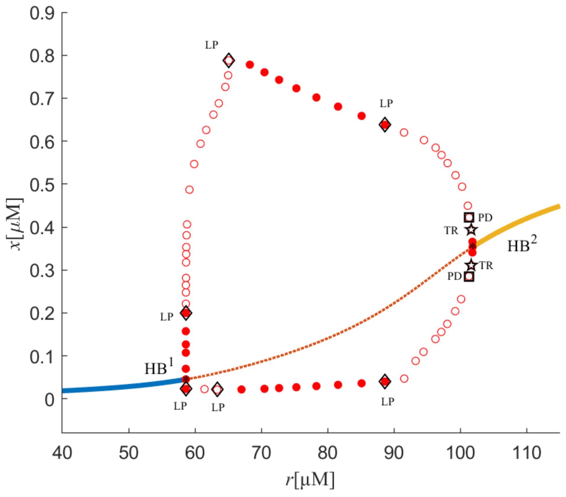
Variations of Ca_tot and Ca_cyt were analyzed from the point of view of bifurcation dynamics. The system presents an equilibrium state and an oscillation state. The equilibrium bifurcation diagram of system (2) is schematically illustrated in Figure 1. In the figure, stable equilibrium points are denoted as the solid line, and unstable equilibrium points are denoted by the dashed line. Additionally, red hollow circles represent unstable limit cycles, and red-filled circles indicate stable limit cycles. Two Hopf bifurcations, namely HB¹ and HB², can also be found with corresponding values of r₁ = 58.61 and r₂ = 101.83. When r passes through r₁ = 58.61 and r₂ = 101.83, two supercritical bifurcations occur in the system.

First, the stability of equilibria is discussed. The stability undergoes a series of variations. To be specific, from r = 0 to 58.61 and from r = 101.83 to 150, there were stable equilibria. Between r = 58.61 and 101.83, there were unstable equilibria. This is followed by a discussion of the stability of limit cycles. A stable limit cycle formed at r = 58.61. When r increased to 58.62, saddle-node bifurcation (LP) of limit cycles occurred, and stable and unstable limit cycles had a meeting at this point. Thus, stable limit cycles became unstable. Similarly, LP of the limit cycles was at r = 65.09 and 89.96. The stability of limit cycles was constantly changing. Limit cycles go from unstable to stable. Then, unstable limit cycles were obtained through r = 89.96. At different values of r, for example, r = 101.8, torus bifurcation (TR) was in the system and period doubling bifurcation (PD) could also be found when r = 101.3. Period doubling bifurcation is a typical approach to chaos, which can be considered as a way to enter chaos from period windows.

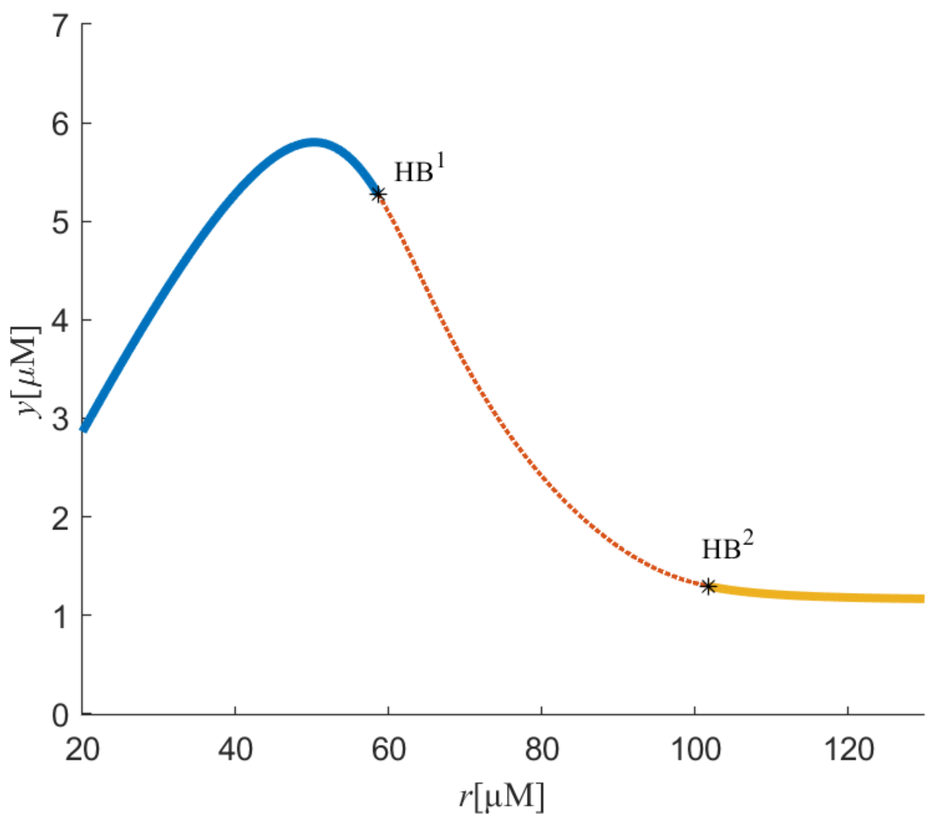
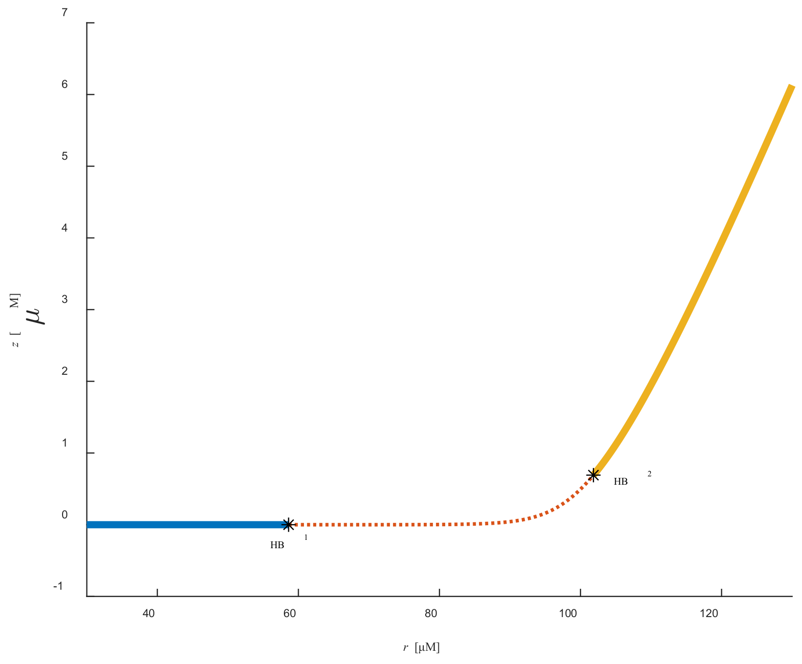
When the limit cycles pass through TR, the stability of the system limit cycles transforms further, and unstable limit cycles of the system turn into stable limit cycles. Torus bifurcation (TR) is a way to cause chaos in the system and is shown in the following images. Figure 2 and Figure 3 represent the bifurcation diagram in the (r, y) and (r, z) planes, respectively. One can easily see that two Hopf bifurcation points appeared due to the variation in parameter r.

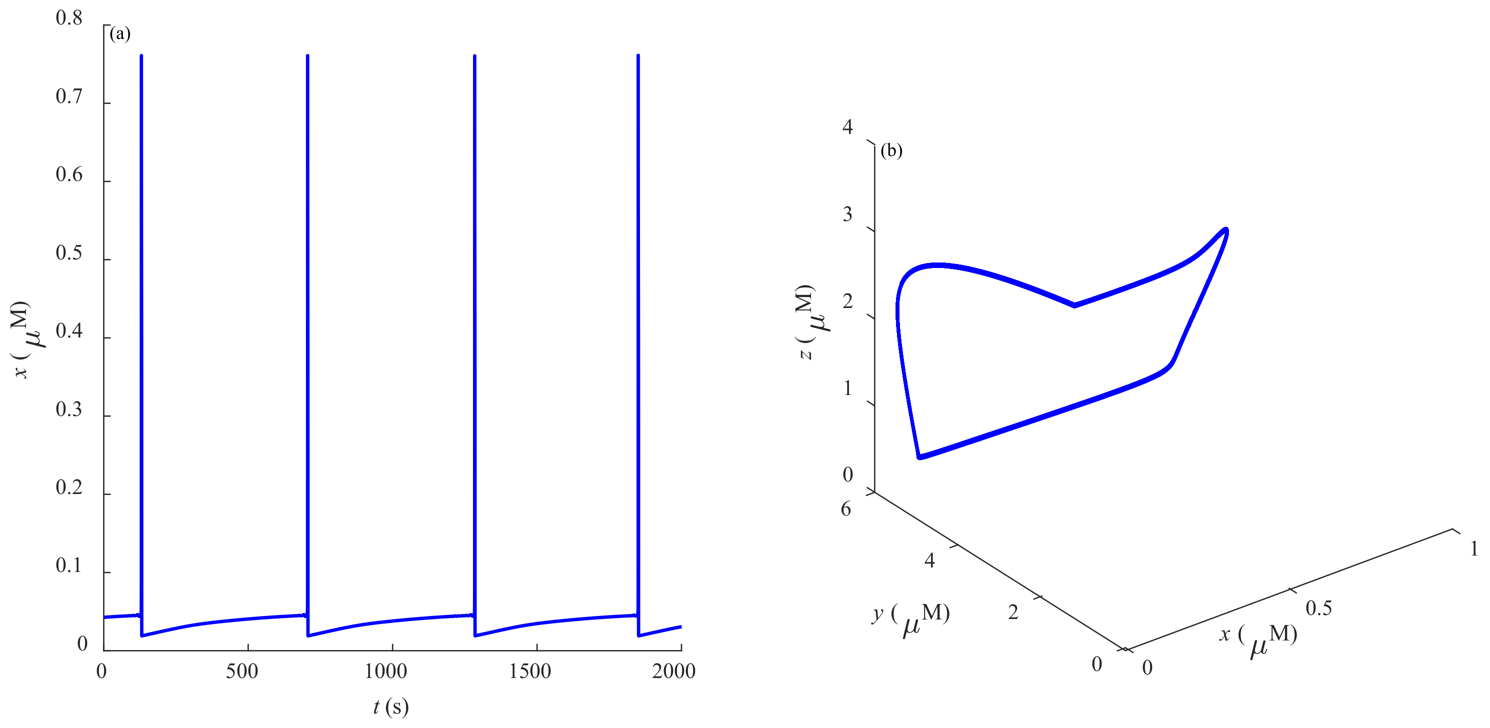
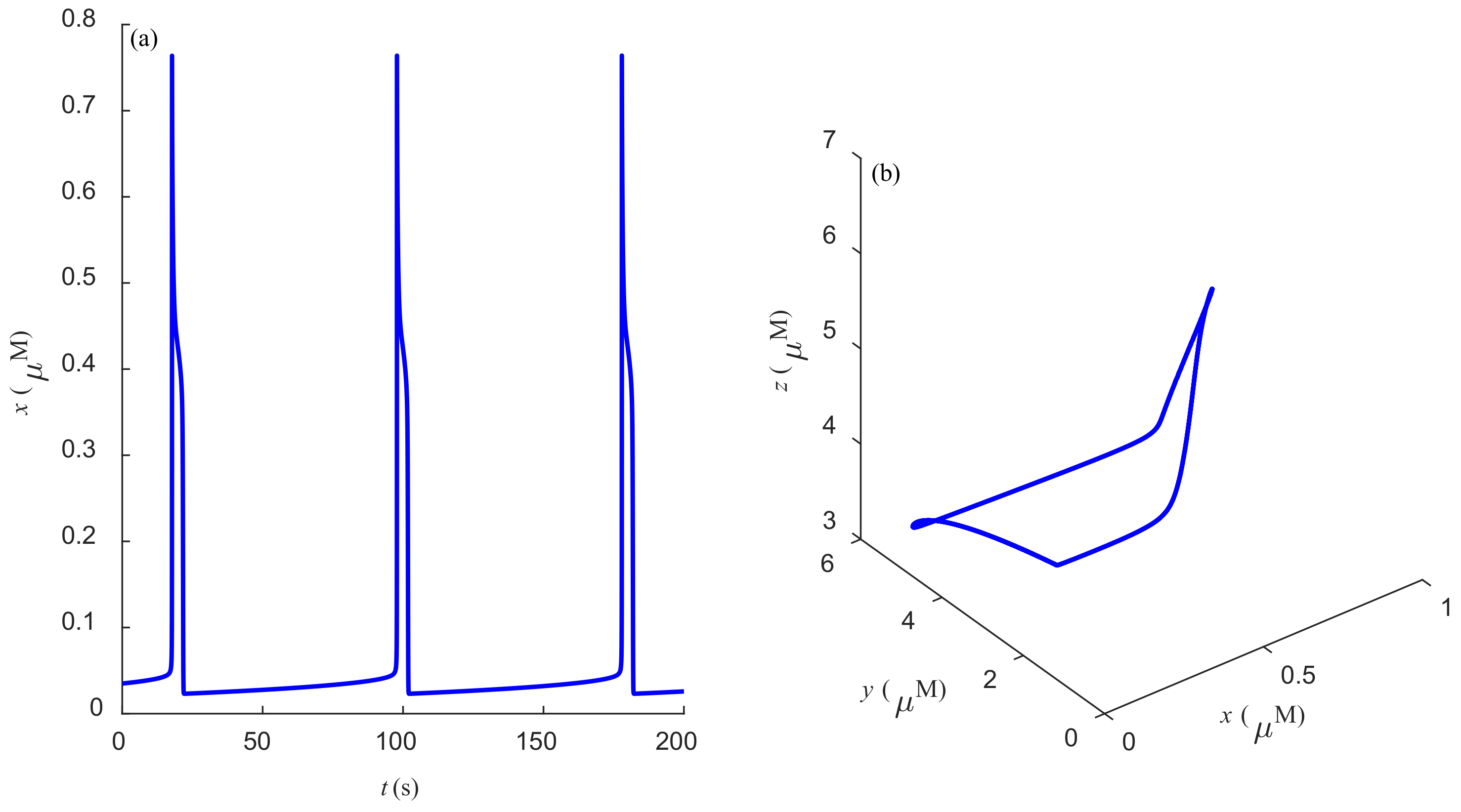
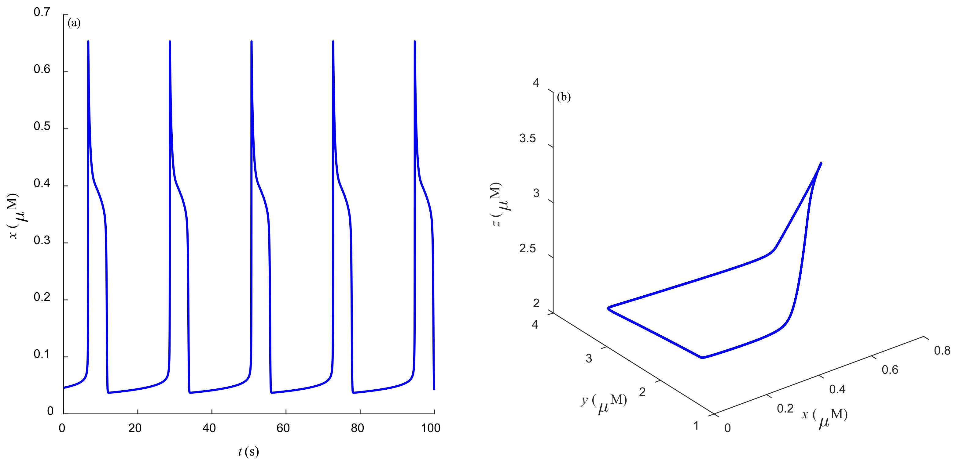
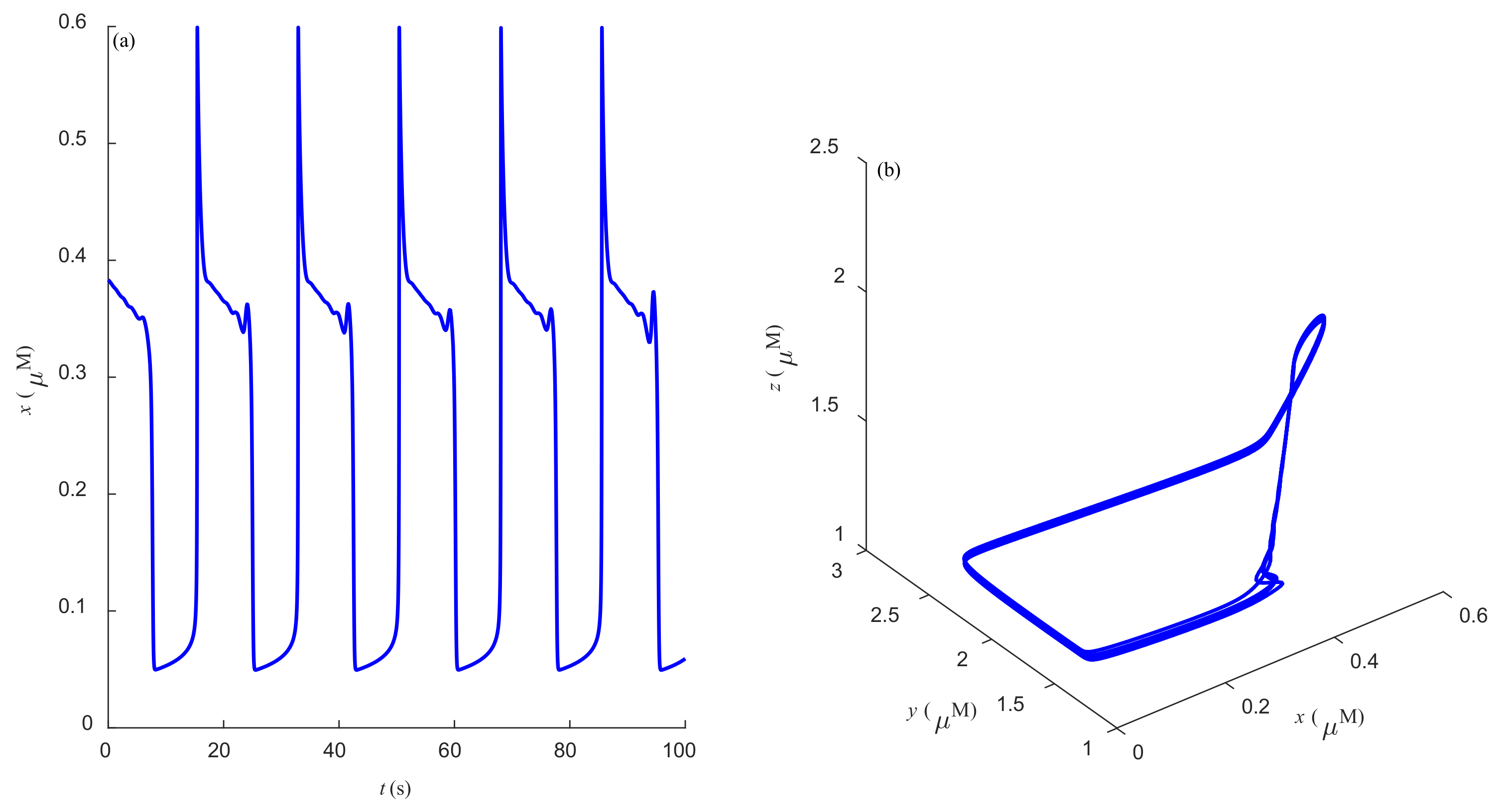
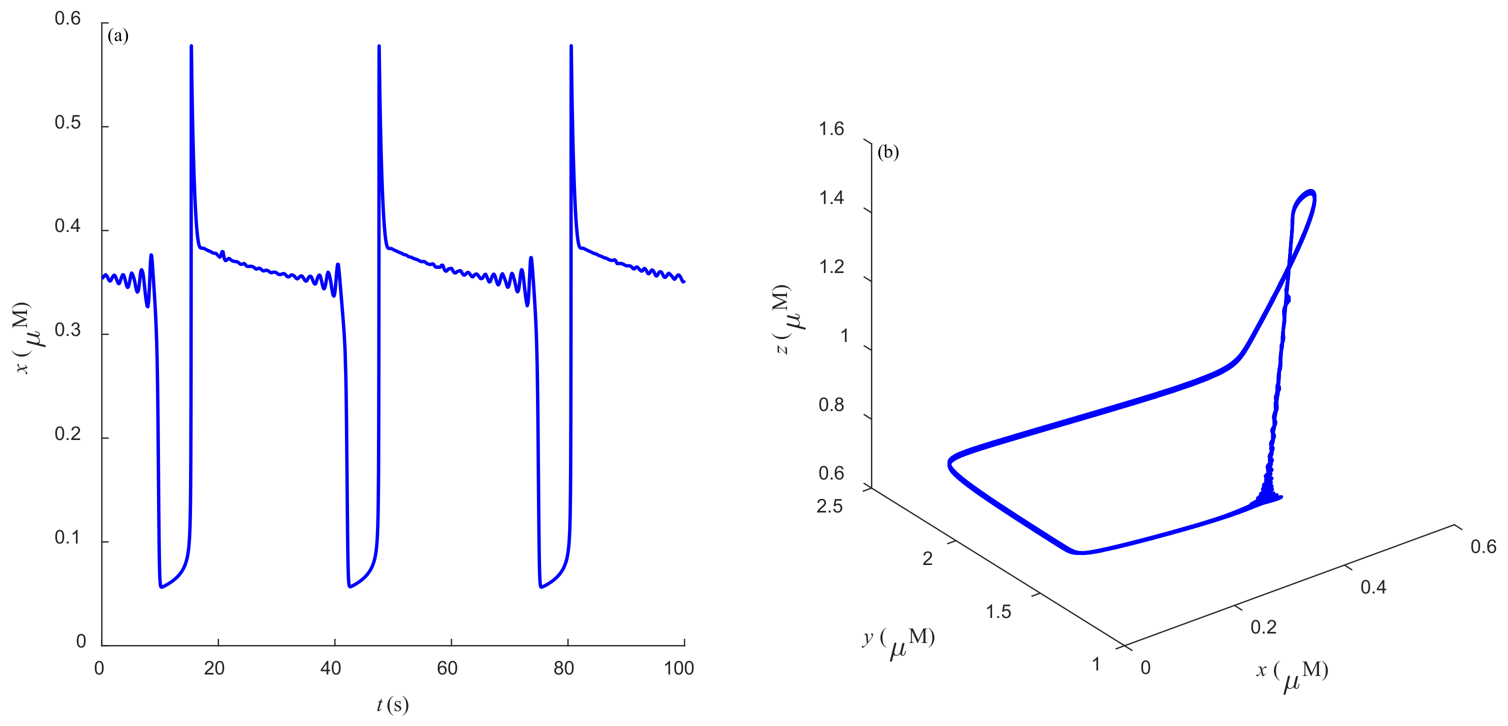
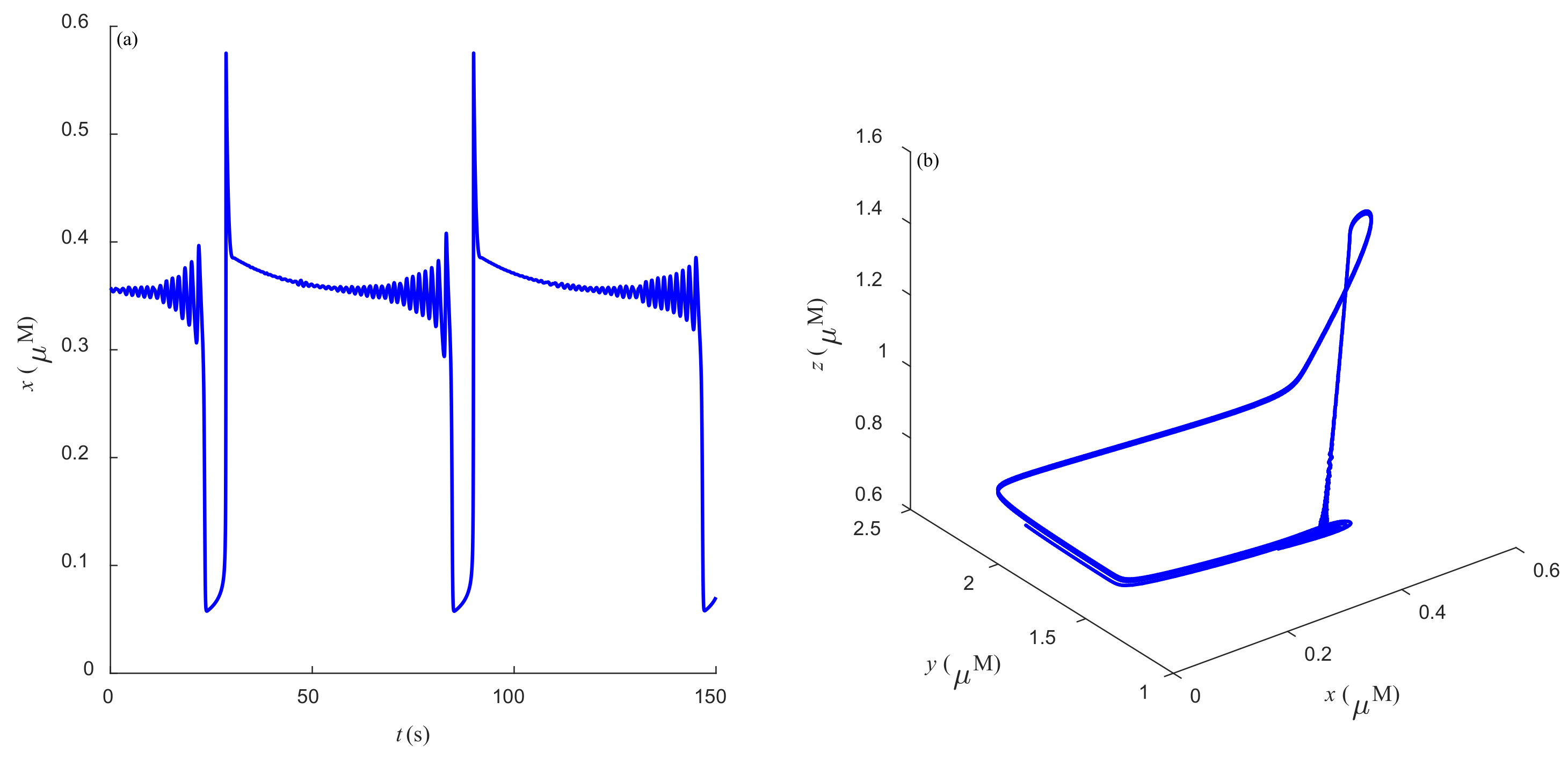
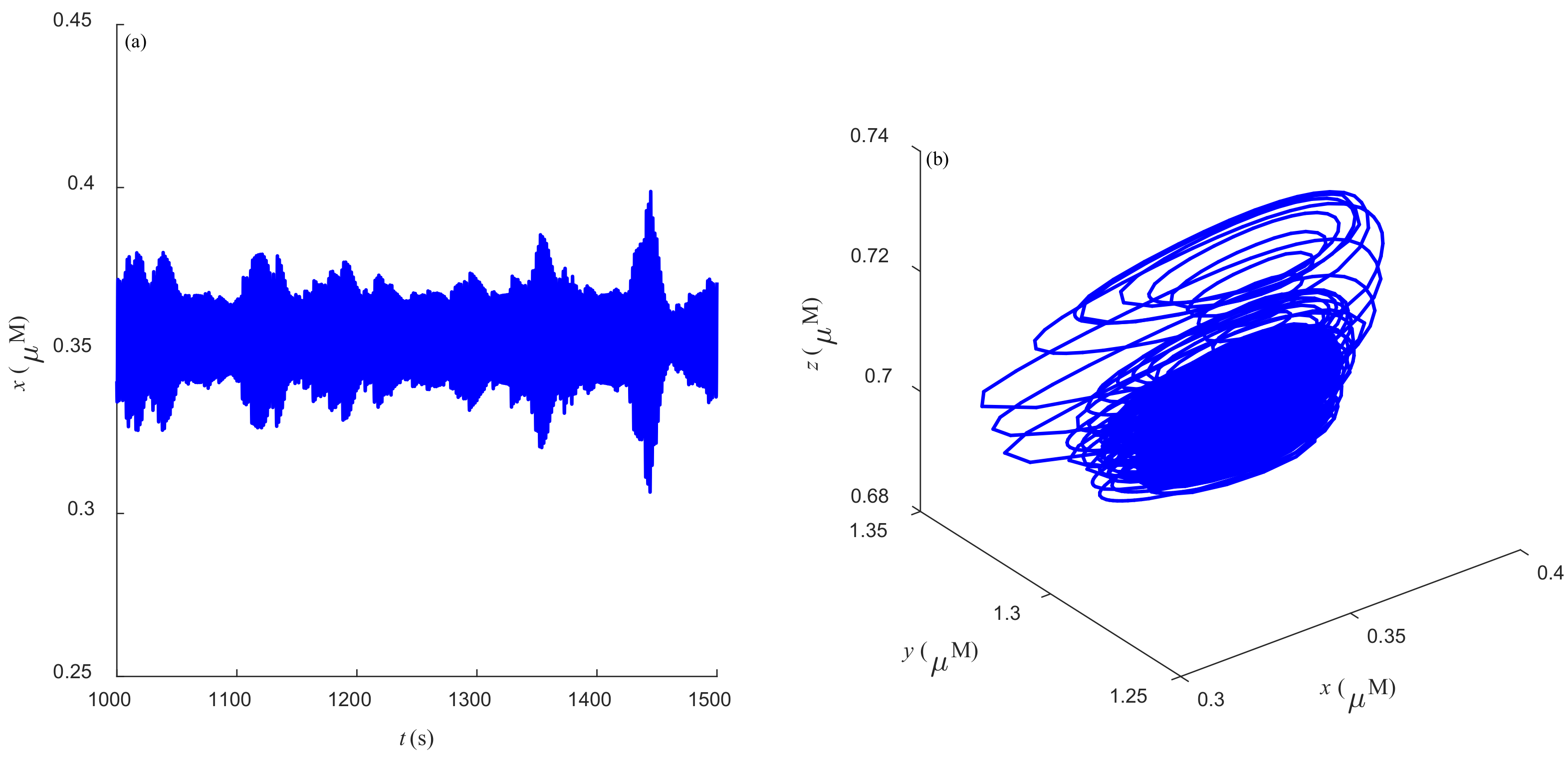
Some dynamic behaviors of system (2) are schematically presented in Figure 4, Figure 5, Figure 6, Figure 7, Figure 8, Figure 9 and Figure 10. Figure 4a, Figure 5a, Figure 6a, Figure 7a, Figure 8a, Figure 9a and Figure 10a represent the temporal evolution for different values of parameter r. Figure 4b, Figure 5b, Figure 6b, Figure 7b, Figure 8b, Figure 9b and Figure 10b correspond to different state trajectories in 3D phase space by varying different values of r. Among these, Figure 4, Figure 5, Figure 6, Figure 8 and Figure 9 represent the regular Ca²⁺ oscillations. Illustrations of chaos can be observed in Figure 7 and Figure 10. These phenomena are abundant and need further study.

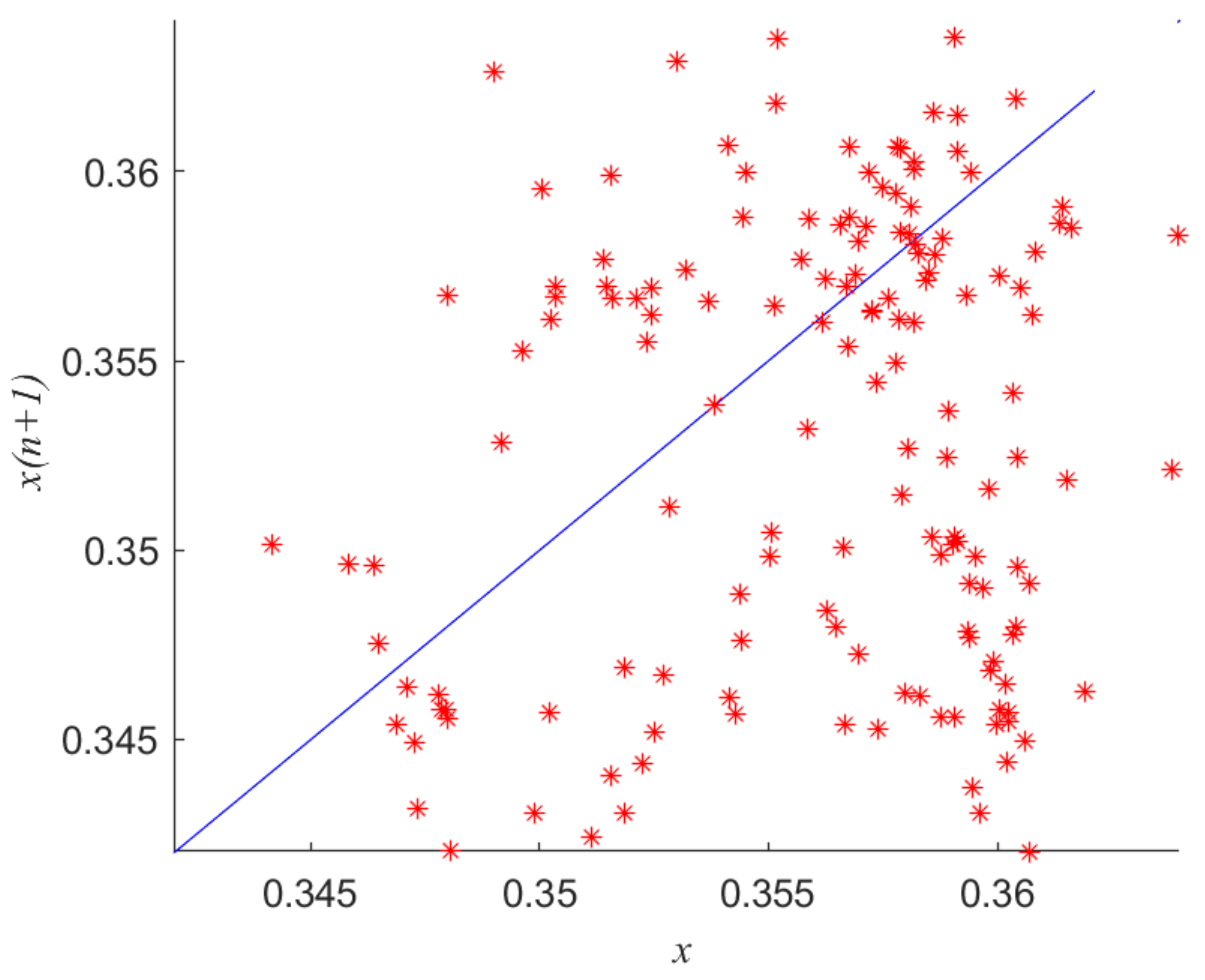
Figure 11 is the return map for when r = 101.8. In the figure, the pioneer points x were compared to the successor points x (n + 1). When the track repeatedly traverses the same section, the points on the left of the section are very scattered. The image shows a scatterplot. Therefore, there is chaos in the system at this point. Furthermore, when the images drawn in Figure 11 were observed together with torus bifurcation (TR) and period doubling bifurcation (PD) in Figure 1 and the sequence diagram of time and phase diagram in Figure 10, we can see that the characteristics of system (2) displayed in these images were consistent and chaos was found in all of these diagrams, further validating the availability of the method.

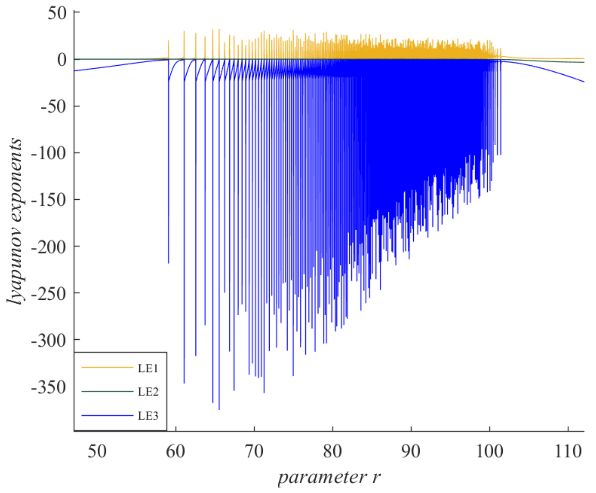
Figure 12 investigates the Lyapunov exponential spectrum of system (2). Lyapunov exponent is a description of the stability of a dynamic system. When the Lyapunov exponent is greater than zero, it means chaos occurs in the system. For n-dimensional continuous dynamical systems $\dot{x}$ = g (x), the system forms an n-dimensional sphere with x₀ as the center and $\Vert \delta$ x(x₀,0) $\Vert$ as the radius when t = 0. With the evolution of time, the sphere deforms into an n-dimensional ellipsoid at time t. Assume that the length of the half-axis in the direction of the ith-axis of the ellipsoid is $\Vert \delta$ x_i (x₀, t) $\Vert$, then the ith-Lyapunov exponent of the system is

$${\lambda }_i=\underset{t\to \infty }{\lim }\frac{1}{t}\ln \frac{\parallel \mathit{\delta }{x}_i(x_0,t)\parallel }{\parallel \mathit{\delta }x(x_0,0)\parallel }.$$

Solving the formula will give the Lyapunov exponent. In Figure 12, the yellow curves represent LE1, the green curves represent LE2, and the blue curves represent LE3. The Lyapunov exponent was more than 0 within a certain parameter range, indicating the presence of chaos in system (2). For example, when r = 101.8, the corresponding Lyapunov exponents were LE1 = 0.1378, LE2 = −0.4361, and LE3 = −27.6405, respectively. LE1 > 0, so the system was in chaos at this point, which is consistent with Figure 1, Figure 10, and Figure 11.

5. Summary

In this study, the stability and bifurcation phenomena of a 3D Ca²⁺ oscillation model were investigated theoretically and simulated numerically. Oscillations of Ca²⁺ in the cytosol, endoplasmic reticulum, and mitochondria were studied using the total concentration of Ca²⁺ in the cytosol, mitochondria, and endoplasmic reticulum as the bifurcation parameter. Two Hopf bifurcation points were obtained after varying the value of the parameter for investigation. There was a stable periodic solution near the supercritical Hopf bifurcation point. The Hopf bifurcation point was the source of oscillation.

After the theoretical analysis of the system, the correctness of the theoretical results was verified by the numerical method. During the numerical simulation, there were some interesting oscillations. In addition to the usual simple oscillations, there were also some Ca²⁺ oscillations of bursting. The peak values and periods of oscillations of different bursting were also different, which may be related to bifurcation. Such findings provided ideas for further research. Moreover, by exploring the bifurcation diagram, the Hopf bifurcation case calculated in this study well matched that of the image. Moreover, there were also limit cycle LP and TR points. Where the system occurred, there was chaos at TR. This provided further insights into the dynamic behavior between the two points where the Hopf bifurcation occurs. In general, the total Ca²⁺ concentration greatly influences the formation and characteristics of Ca²⁺ oscillations in cells.

Some of the special phenomena found above need to be explored in more detail. Future works should select different models, explore different models, and conduct in-depth research. In addition, in many intracellular dynamic models, time delay has a certain effect on the dynamic behavior of cells. However, the model established in this study did not consider the effect of time delay. Therefore, in future works, the study of cell models with time delay is also worth considering.