
Quasi-Periodic Oscillations of Roll System in Corrugated Rolling Mill in Resonance

Abstract
:1. Introduction
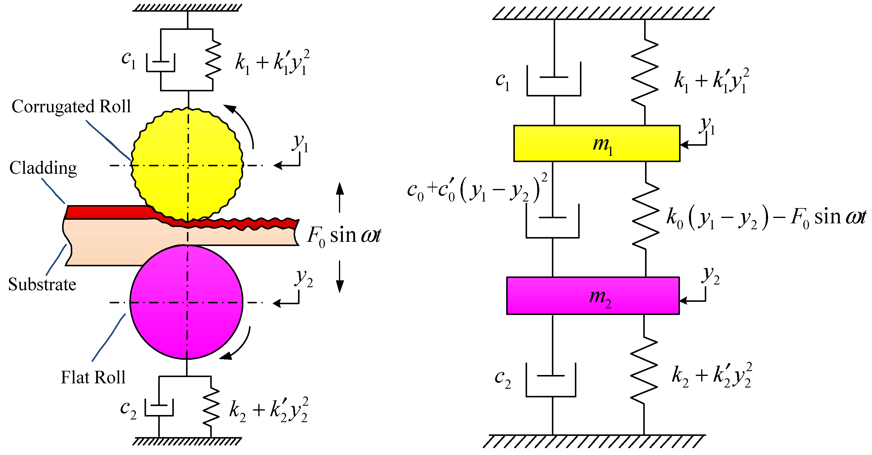
2. The Mechanical Model and Dynamic Equation of Corrugated Rolling Mill
3. The Poincaré Map
4. Neimark-Sacker Bifurcation in Resonance
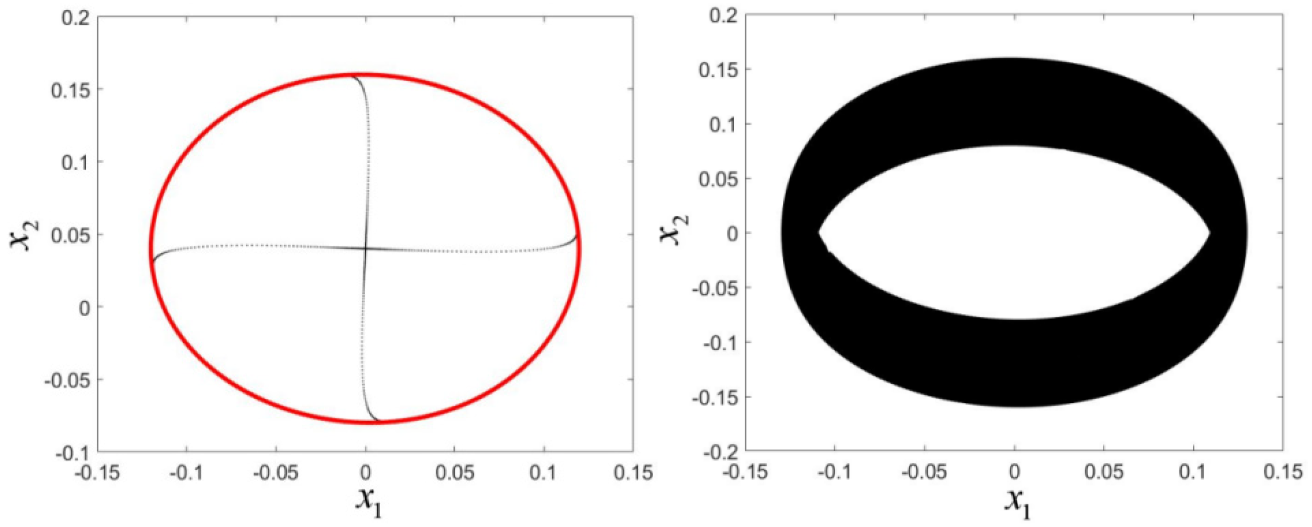
4.1. 1:3 Resonance
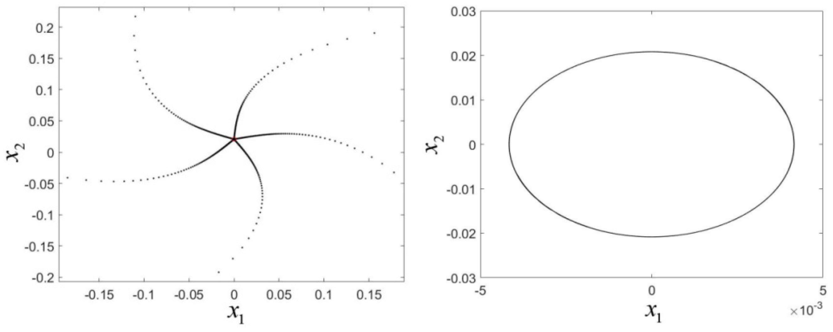
4.2. 1:4 Resonance
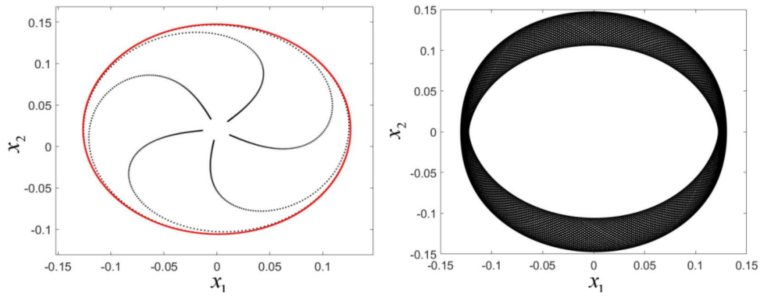
4.3. 1:5 Resonance
5. Conclusions
Author Contributions
Funding
Institutional Review Board Statement
Informed Consent Statement
Data Availability Statement
Acknowledgments
Conflicts of Interest
References
- Johnson, R.E.; Qi, Q. Chatter dynamics in sheet rolling. Int. J. Mech. Sci. 1994, 36, 617–630. [Google Scholar] [CrossRef]
- Swiatoniowski, A. Interdependence between rolling mill vibrations and the plastic deformation process. J. Mater. Process. Technol. 1996, 61, 354–364. [Google Scholar] [CrossRef]
- Yarita, I.; Furukawa, K.; Seino, Y. Analysis of chattering in cold rolling for ultrathin gauge steel strip. Trans. Iron Steel Inst. Jpn. 1978, 18, 1–10. [Google Scholar] [CrossRef]
- Kapil, S.; Eberhard, P.; Dwivedy, S.K. Nonlinear dynamic analysis of a parametrically excited cold rolling mill. J. Manuf. Sci. Eng. 2014, 136, 041012. [Google Scholar] [CrossRef]
- Li, H.G.; Wen, B.C. Nonlinear vibrations of self-excited vibration systems with clearances and oscillating boundaries. J. Vib. Eng. 2000, 13, 122–127. [Google Scholar]
- Huang, H.D.; Zang, Y. Analysis nonlinear friction caused of self-excited vibration of main drive system on rolling mill. Coal Technol. 2012, 31, 222–224. [Google Scholar]
- Hou, D.X.; Liu, B.; Shi, P.M.; Liu, S. Bifurcation of piecewise nonlinear roll system of rolling mill. J. Vib. Shock 2010, 29, 132–135. [Google Scholar]
- Hou, D.X.; Liu, B.; Shi, P.M.; Liu, F.; Liu, Y.J. Vibration characteristics of 2 DOF nonlinear torsional vibration system of rolling mill and its conditions of instability. J. Vib. Shock 2012, 31, 32–36. [Google Scholar]
- Liu, S.; Li, X.; Li, Y.Q.; Li, H.B. Stability and bifurcation for a coupled nonlinear relative rotation system with multi-time delay feedbacks. Nonlinear Dyn. 2014, 77, 923–934. [Google Scholar] [CrossRef]
- Liu, S.; Wang, Z.L.; Wang, J.J.; Li, H.B. Sliding bifurcation research of a horizontal–torsional coupled main drive system of rolling mill. Nonlinear Dyn. 2016, 83, 441–455. [Google Scholar] [CrossRef]
- Zhou, X.M.; Hao, Y.K.; Cong, W.T.; Wei, Z.B.; Wen, G.D. Flutter analysis of cold tandem rolling mills based on gradient boosted decision tree. J. Vib. Shock 2021, 40, 154–158. [Google Scholar]
- Qian, C.; Sun, R.S.; Zhang, L.L.; Bai, Z.H.; Hua, C.C. Coupled vibration model and influencing factors analysis of tandem cold rolling mill. J. Mech. Eng. 2021, 57, 208–216. [Google Scholar]
- Qi, J.B.; Wang, X.X.; Yan, X.Q. Influence of mill modulus control gain on vibration in hot rolling mills. J. Iron Steel Res Int. 2020, 27, 528–536. [Google Scholar] [CrossRef]
- Chatterjee, S.; Mallik, A.K. Bifurcations and chaos in autonomous self-excited oscillators with impact damping. J. Sound Vib. 1996, 191, 539–562. [Google Scholar] [CrossRef]
- Budd, C.; Dux, F.; Cliffe, A. The effect of frequency and clearance variations on single-degreeof-freedom impact oscillators. J. Sound Vib. 1995, 184, 475–502. [Google Scholar] [CrossRef]
- Cui, J.F.; Zhang, W.Y.; Liu, Z. On the limit cycles, period-doubling, and quasi-periodic solutions of the forced Van der Pol-Duffing oscillator. Numer. Algorithms 2018, 78, 1217–1231. [Google Scholar] [CrossRef]
- Wen, G.; Xu, H.; Chen, Z. Anti-controlling quasi-periodic impact motion of an inertial impact shaker system. J. Sound Vib. 2010, 329, 4040–4047. [Google Scholar] [CrossRef]
- Guo, Y.; Xie, J.H. N-S Bifurcation of an oscillator with dry friction in 1:4 strong resonance. Appl. Math. Mech. Engl. 2013, 34, 27–36. [Google Scholar] [CrossRef]
- Kuznetsov, Y.A. Element of Applied Bifurcation Theory, 2nd ed.; Springer: New York, NY, USA, 1998. [Google Scholar]
- Iooss, G. Bifurcation of Maps and Applications; Mathematical Studies, 36; North-Holland: Amsterdam, The Netherlands, 1979. [Google Scholar]


Publisher’s Note: MDPI stays neutral with regard to jurisdictional claims in published maps and institutional affiliations. |
© 2021 by the authors. Licensee MDPI, Basel, Switzerland. This article is an open access article distributed under the terms and conditions of the Creative Commons Attribution (CC BY) license (https://creativecommons.org/licenses/by/4.0/).
Share and Cite
He, D.; Xu, H.; Wang, T.; Wang, Z. Quasi-Periodic Oscillations of Roll System in Corrugated Rolling Mill in Resonance. Mathematics 2021, 9, 3201. https://doi.org/10.3390/math9243201
He D, Xu H, Wang T, Wang Z. Quasi-Periodic Oscillations of Roll System in Corrugated Rolling Mill in Resonance. Mathematics. 2021; 9(24):3201. https://doi.org/10.3390/math9243201
Chicago/Turabian StyleHe, Dongping, Huidong Xu, Tao Wang, and Zhihua Wang. 2021. "Quasi-Periodic Oscillations of Roll System in Corrugated Rolling Mill in Resonance" Mathematics 9, no. 24: 3201. https://doi.org/10.3390/math9243201