1. Introduction
Nonlinear oscillators appear in many applied sciences, involving mechanical engineering, mechanics, chemistry, biology and physics, and have a wide range of engineering backgrounds. The Duffing [
1,
2], van der Pol [
3,
4] and Rayleigh [
5,
6] oscillators are well-known models of nonlinear systems in physics and mechanics.
In the wake of the rapid development of the economy and technology, the continuous emergence of new structures and construction technologies and the increasing aesthetic needs of the public, pedestrian bridges, stadiums, floors and other structures are becoming increasingly slender. However, these structures are subjected to walking load, so it is easy to produce a large-amplitude vibration. The modified hybrid van der Pol-Rayleigh (MHVR) system proposed by Erlicher et al. [
7] is a kind of typical self-excited oscillation system, which can be suitably applied to the pedestrian walking lateral force model.
As a combination of the two oscillators, the dynamic behavior of the van der Pol-Rayleigh system has attracted extensive attention. Tang et al. [
8] studied the vibration response and its generation mechanism in the van der Pol-Rayleigh system under slow-varying periodic excitation, and analyzed the excitation hysteresis behavior and its generation mechanism of the system. Saha et al. [
9] classified the van der Pol oscillator and Rayleigh oscillator into the general form of the Liénard-Levinson-Smith (LLS) system, and thus design a generalized van der Pol and Rayleigh oscillator family system with multiple limit cycles. Hasegawa [
10] studied the Jarzynski equality in van der Pol and Rayleigh oscillators to which a ramp force with a duration τ is applied. In the τ range, the Jarzynski equality (JE) is basically valid, but not completely satisfied. The work distribution function (WDF) uses a u-shaped structure with large damping parameters. Jerzy [
11] studied the interactions between two parametrically coupled, self-excited oscillators. The different types of motion were classified by Lyapunov’s exponent criterion. Veskos and Demiris [
12] studied the effects of different lower-level building blocks of a robotic swinging system using the van der Pol and Rayleigh oscillators. The similarities and differences between these oscillators were analyzed. Chen et al. [
13] studied the dynamics of a hybrid van der Pol-Rayleigh oscillator and discovered new dynamics that are different from van der Pol and Rayleigh oscillators. At the same time, the van der Pol-Rayleigh system is also widely used in mechanics, electronic circuits, biomechanics and other engineering areas. For example, Bartkowiak and Woernle [
14] adjusted the parameters of the van der Pol-Rayleigh oscillator to the given harmonic base excitation, and then added them to the linear multi-body system. After adjusting the amplitude and phase shift, the vibration absorption and energy collection tasks were completed. Chen et al. [
15] used the multi-scale method to decouple the van der Pol-Rayleigh equation and applied the discussion results to the dynamic model of the side-coupling system of a footbridge—a flexible footbridge.
The fast–slow coupling systems can often cause bursting oscillation, which is an important dynamic behavior. The fast–slow analysis method [
16] first proposed by Rinzelis can be used to reveal the generation mechanism of the bursting response. The bursting oscillation [
17,
18,
19,
20,
21] is composed of large and small oscillations alternately in a given period. Generally speaking, the large-amplitude oscillation is called the spiking state motion, and its trajectory moves in the large-amplitude limit cycle vector field. The small-amplitude oscillation is called the quiescent state motion and its trajectory moves within the small-amplitude limit cycle vector field or the equilibrium attraction region.
In this paper, we will analyze the dynamic response behavior of the van der Pol-Rayleigh system, reveal the mechanism of vibration generation in different modes and discuss the transition process among the different types of attractors in the process of rapid change. In practical engineering, the results of the discussion can be used to reasonably utilize or avoid these large vibrations in advance, so as to improve the stability of the equipment, prolong the service cycle and increase the economic and social benefits.
The remainder of this paper is organized as follows. In
Section 2, the stability and bifurcation behavior of the equilibrium point of the system are analyzed. In
Section 3, the fast subsystem is simulated numerically and analyzed with or without external excitation. In
Section 4, the vibration behavior and its generation mechanism of the system in different modes are analyzed. In
Section 5, we draw the conclusions.
2. The System Model and Bifurcation Analysis
2.1. The System Model
The model equation in [
7] is:
where
is a real function,
is the natural frequency of the system,
is the periodic excitation frequency,
is the periodic excitation amplitude,
,
,
,
are parameters, and
,
,
,
,
,
. Obviously, the system is the Rayleigh oscillator when
; the system is the van der Pol oscillator when
. Therefore, this is a coupling van der Pol-Rayleigh system.
Let
, and Equation (1) can become:
When and , we can view as the slow variable. In any period corresponding to the natural frequency, the excitation term changes between and , obviously , so the change in in any period of the natural frequency is very small. Regarding as a generalized parameter of Equation (2), Equation (2) can be called a generalized autonomous system with respect to accordingly. We regard the generalized autonomous system (2) as the fast subsystem corresponding to the fast variable and , while treating as the corresponding slow subsystem.
2.2. Bifurcation Analysis
To further reveal the mixed-mode vibration behavior of Equation (2), its bifurcation behavior with respect to the slow variable will be discussed.
2.2.1. Equilibrium Analysis and Fold Bifurcation
The equilibrium point of the system is
, and the Jacobian matrix of the linear system derived at
is
The corresponding characteristic equation is
where
,
. Its eigenvalues are
.
When , namely or , the equilibrium point is stable; conversely, when , namely , the equilibrium point is unstable. At the same time, when , namely or , the equilibrium point is a stable node; when , namely , the equilibrium point is an unstable node. When , namely or , the equilibrium point is a stable focus; when , namely or , the equilibrium point is an unstable focus.
Because , the characteristic Equation (4) has no zero eigenvalue, and the system (2) has no fold bifurcation.
2.2.2. Hopf Bifurcation
Theorem 1. Ifis the bifurcation parameter of the fast subsystem (2), the sufficient and necessary conditions for the equilibrium point of the fast subsystem to produce Hopf bifurcation atare
(1);
(2).
Proof of Theorem 1. The condition of the characteristic Equation (4) has a pair of pure imaginary roots: , .
Because , we can obtain that .
When , we can determine that . Thus, Equation (2) may cause the Hopf bifurcation.
The existence of the Hopf bifurcation must also satisfy the transversal condition . The transversal condition of the Hopf bifurcation is proven below.
Taking the partial derivative of both sides of the characteristic Equation (4) with respect to
, we obtain
Let
, and substitute it into Equation (5) to obtain
Separate the real part of
, and substitute
into Equation (6) to obtain
Thus, when , determine . Therefore, Equation (2) will cause the Hopf bifurcation when . □
2.2.3. The First Lyapunov Coefficient
In order to judge the bifurcation direction and the stability of the Hopf bifurcation, the first Lyapunov coefficient
[
22] of the system is considered. Firstly, we will shift
to the original point
, and the transformation of coordinates is
Substitute Equation (8) into Equation (2), and then use
and
to replace
and
, so Equation (2) can be converted into
Next, transform Equation (9) into
where
Substitute
into characteristic Equation (5), and obtain
,
. Thus,
The eigenvector of
corresponding to
is called
, and the eigenvector of
corresponding to
is called
. In other words,
,
,
. Thus, we can calculate the following:
is a smooth function that can be expanded as
where
and
are bilinear functions, and
After calculation, we can obtain
Then, after a series of calculations, we obtain
In [
22], we can see that when
, the system experiences the subcritical Hopf bifurcation and an unstable limit cycle is obtained; when
, the system experiences the supercritical Hopf bifurcation and a stable limit cycle is obtained; when
, the system experiences the codimensional 2 degenerate Hopf bifurcation.
Now, fixing the parameters
,
,
,
, we can obtain
Thus, when , , the system experiences the supercritical Hopf bifurcation and the resulting limit cycle is stable. When and , , the system experiences the subcritical Hopf bifurcation and the resulting limit cycle is unstable.
2.3. Bifurcation Curve
Fixing the parameters
,
,
,
,
,
, the bifurcation diagram of the fast subsystem (2) with respect to
can be drawn, as shown in
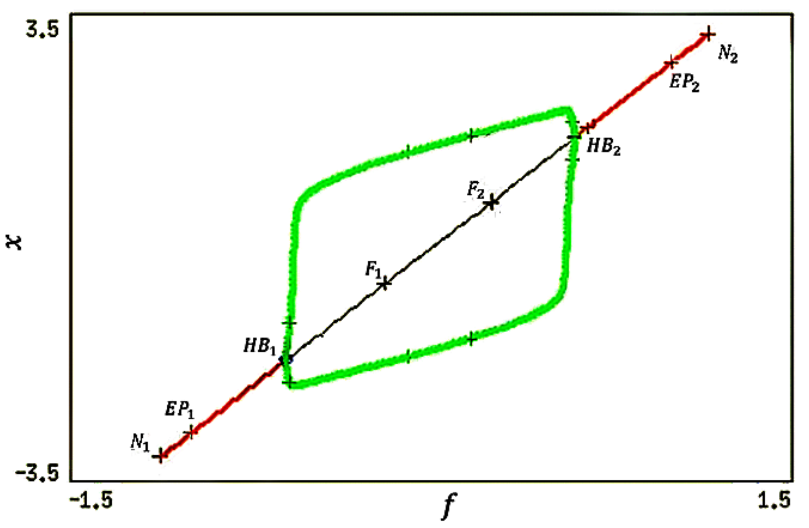
Figure 1. The red solid line indicates that the equilibrium is stable, the black solid line indicates that the equilibrium point is unstable, and the green solid line indicates that the system has a stable limit cycle; these are consistent with the actual characteristics of the van der Pol-Rayleigh system.
In
Figure 1,
and
are Hopf bifurcation points;
and
are limit points, and also are the saddle of the system, called the turning point. There are four different equilibrium lines distributed on the equilibrium line
. The first kind of equilibrium lines are from the point
to the point
and from the point
to the point
, and the points on this kind of line are stable nodes. The second kind of equilibrium lines are from the point
to the point
and from the point
to the point
, and the points on this kind of line are stable focuses. The third kind of equilibrium lines are from the point
to the point
and from the point
to the point
, and the points on this kind of line are unstable focuses. The fourth kind of equilibrium line is from the point
to the point
, and the points on this kind of line are unstable nodes.
The images drawn by the software XPPAUT are consistent with the theoretical analysis, and the type and stability of the system equilibrium point discussed by the linear characteristic equation derived from the system are consistent with the results obtained by the actual software application.
3. Numerical Simulation of the System
Fixing the parameters , , , , the vibration behavior of the system before and after external excitation is given by numerical simulation.
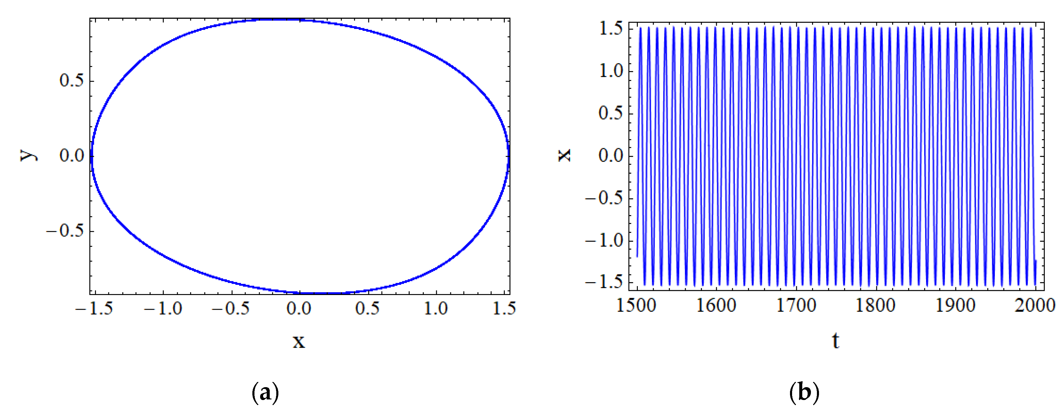
When
, the system degenerates to the original MHVDR system. The numerical simulation shows that the system causes a simple periodic vibration, as shown in
Figure 2. The phase plane portrait is a closed elliptical trajectory. Thus, it is also verified that the system displays periodic motion from another aspect. From
Figure 2, we can see that the system trajectory hardly changes when
changes.
When the slow-varying external excitation
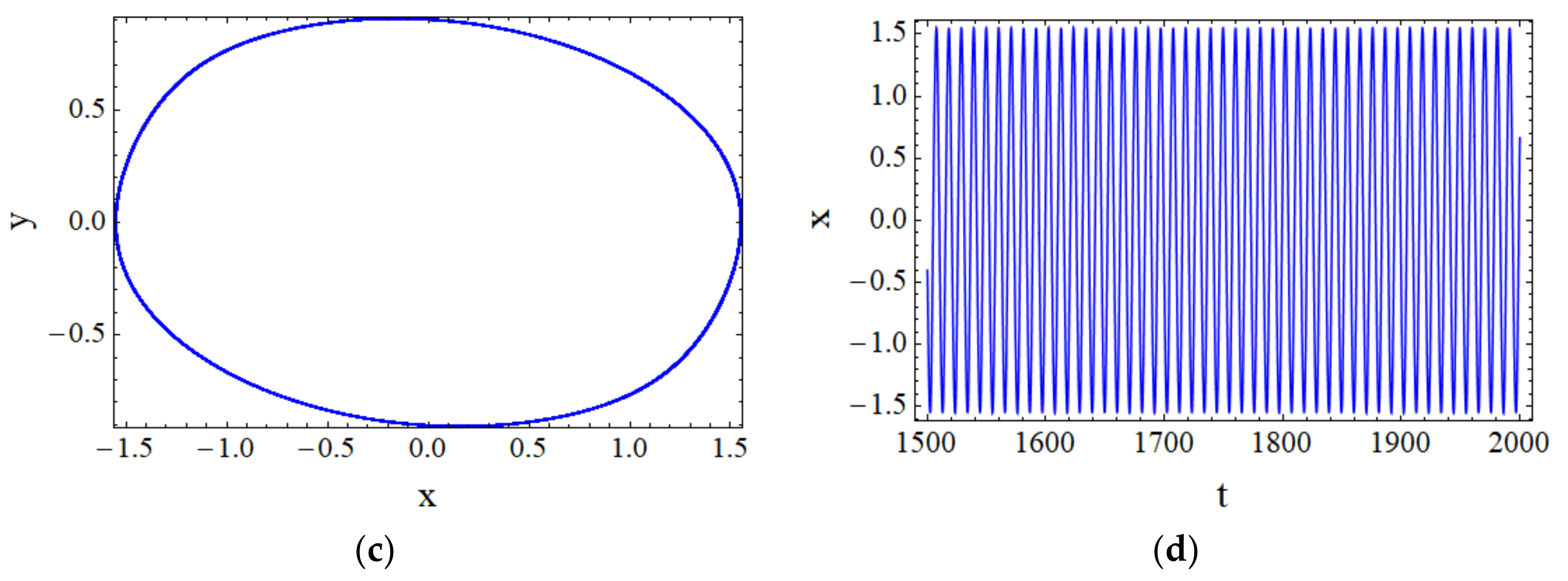
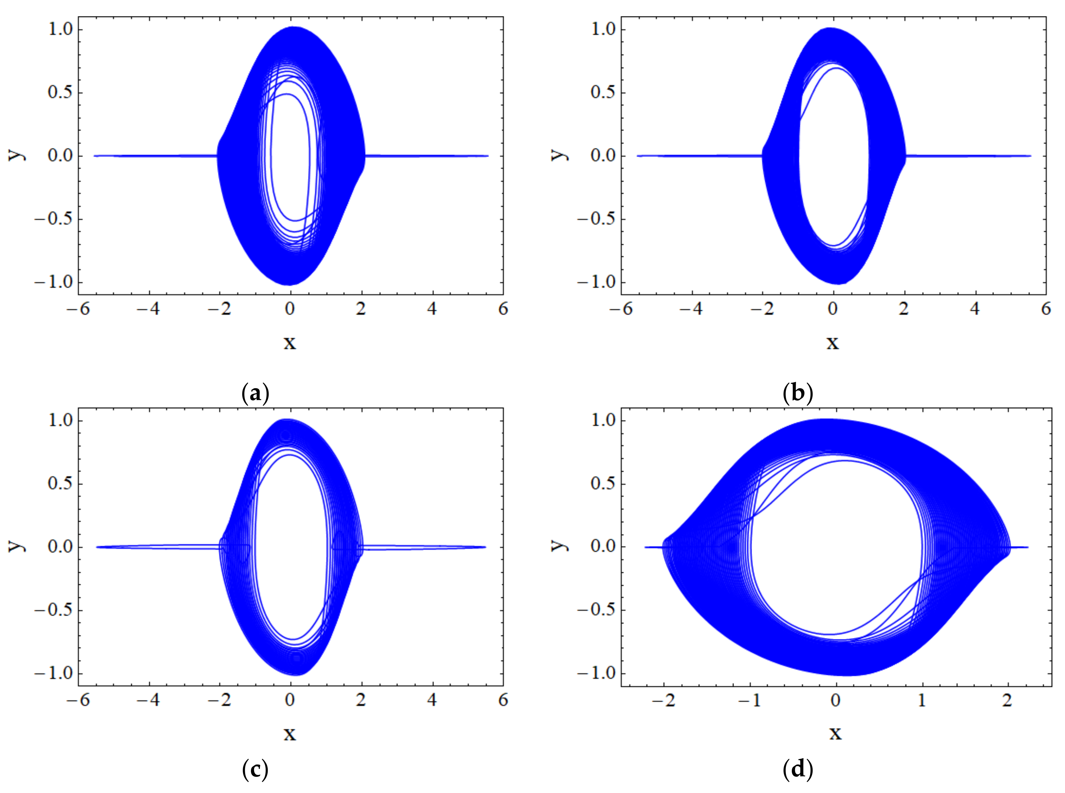
is applied to the system, the system presents a relatively complex vibration mode, which is not a single vibration mode within a period, as shown in
Figure 3 and
Figure 4. The vibration mode is composed of large and small oscillations alternately in a period.
Comparing (a) with (b) in
Figure 3, the system trajectory hardly changes when
changes. Comparing (b) with (c) in
Figure 3, the period becomes short when
changes. Finally, comparing (c) with (d) in
Figure 3, when
changes from
to
, its vibration mode is still in the form of bursting oscillation, but it is more violent than the spiking state in
Figure 3c. Therefore, it can be seen that the parameters have a certain influence on the bursting oscillation of the system.
4. Mechanism of Vibration Generation in Different Modes
Regarding the external excitation as the slow-varying bifurcation parameter of the fast subsystem, the transformation phase portrait of the fast variables and the slow variables is drawn. To further reveal the bifurcation mechanism of the bursting oscillation, the transformation phase portrait is superimposed with the bifurcation diagram of the fast subsystem about . Thus, we can further study the vibration response behavior of the system visually, analyze the transfer process between multiple attractors in the system, discuss the mechanism of the bursting phenomenon generated and further explore the influence of external excitation amplitude on the fast subsystem.
Fixing the parameters , , , , , , we take the excitation amplitudes as , , , and respectively. Thus, the time history diagrams and the superposition diagrams of the system are drawn.
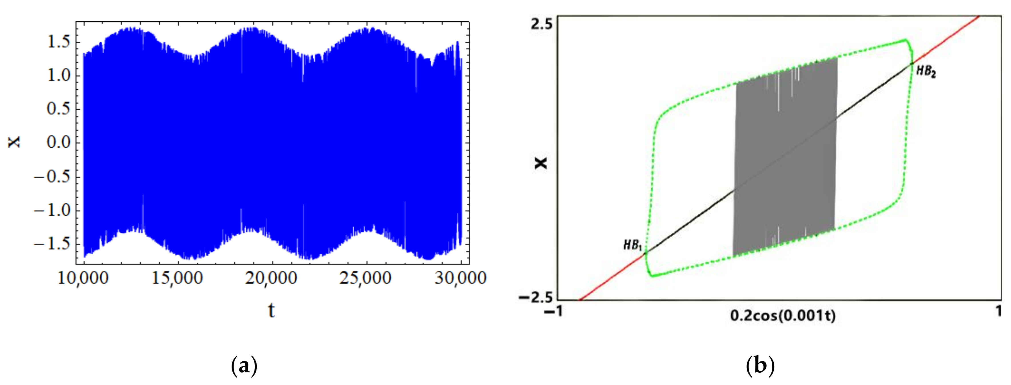
4.1. The Mode of
Letting
, we draw the time history diagram and the superposition diagram of the system, as shown in
Figure 5.
In
Figure 5a, the system presents a large vibration mode of periodic vibration with two frequency coupling. One of the frequencies is the external excitation frequency
, and the other frequency is close to
. The system vibrates at constant amplitude and high frequency in accordance with the natural frequency of the fast subsystem in each slow-varying period, which is presented as the spiking state motion.
Figure 5b is the superposition graph drawn, and
changes within the interval
. At this time, the system trajectory is only within the attraction domain of the limit cycle attractor, the system presents the spiking state motion of high frequency vibration, and the vibration amplitude is the same as that of the limit cycle.
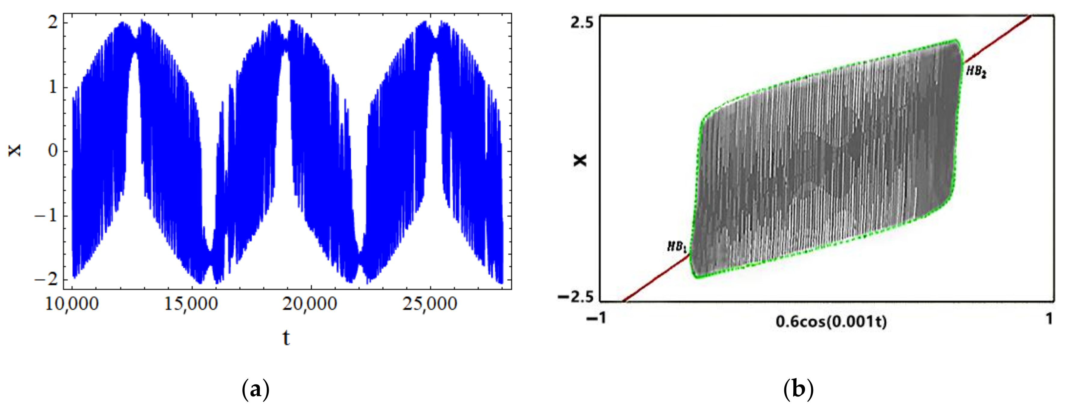
4.2. The Mode of
When
increases, the vibration state of the system becomes different. When
, the time history diagram and the superposition diagram of the system are drawn, as shown in
Figure 6.
In
Figure 6a, we show that the system still presents the spiking state. However, in each slow-varying period, the amplitudes of the system are not the same, but there are distinct differences. Thus, it can be judged that the system changes from constant-amplitude, high-frequency vibration to variable-amplitude, high-frequency vibration.
It can be seen from
Figure 6b that the system trajectory spreads towards both sides of the limit cycle. When
is the Hopf bifurcation point
, the system trajectory covers the whole region. Moreover, the amplitude of the system also changes. As the amplitude of the limit cycle decreases, the amplitude of the system is no longer the original high-frequency vibration amplitude.
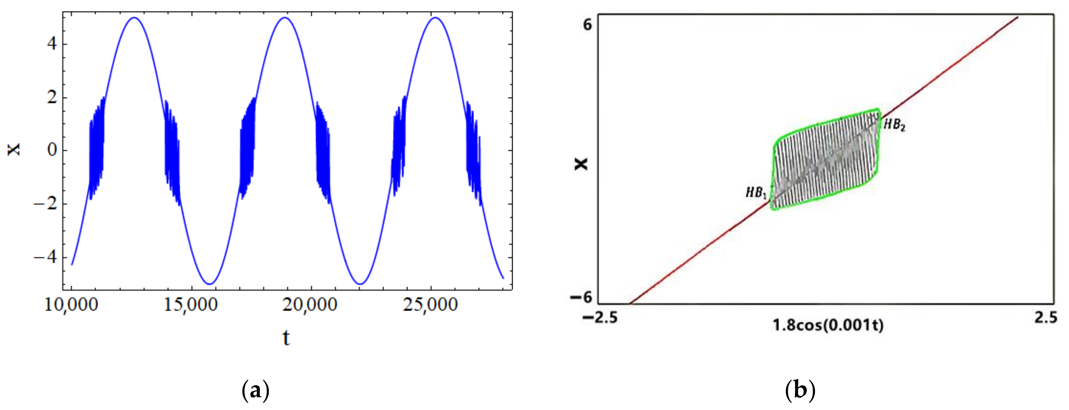
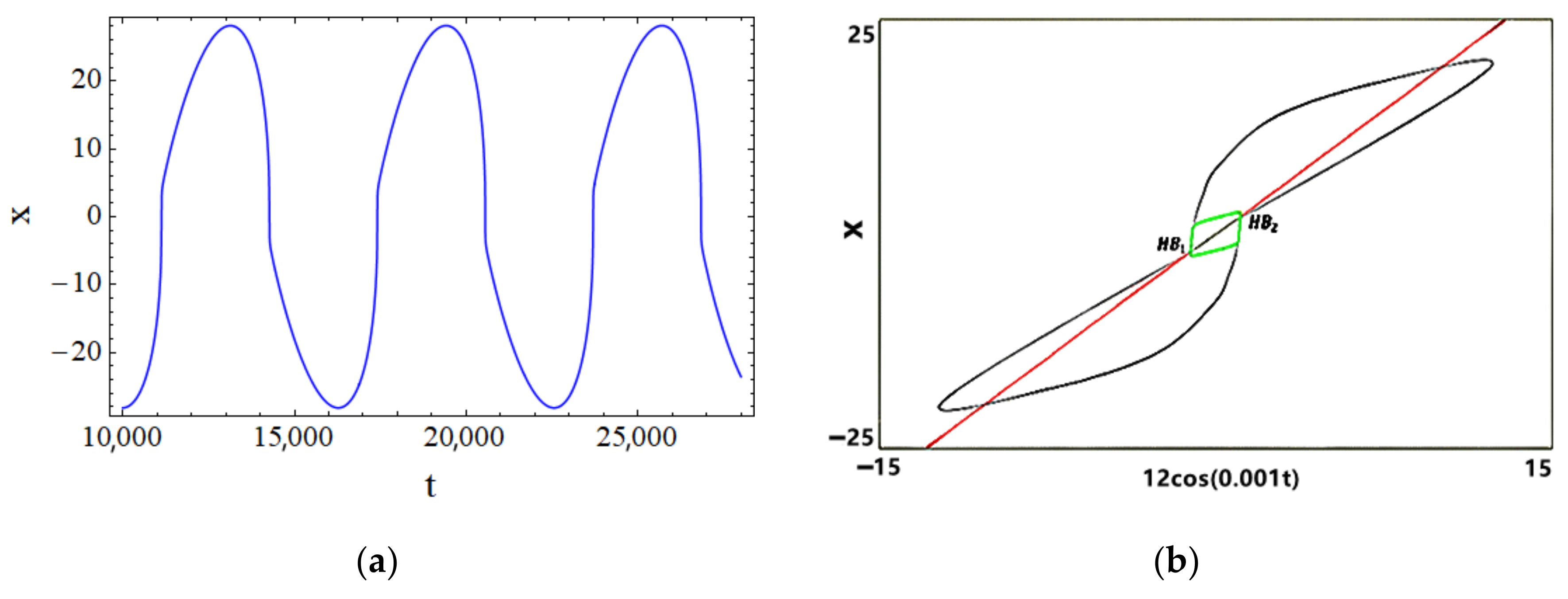
4.3. The Mode of
When
continues to increase, the system can display the situation of the coexistence of the limit cycle attractor and stable equilibrium attractor, resulting in the “bistable state” situation.
Figure 7 plots the time history diagram and the superposition diagram of the system when the excitation amplitude
increases to
. At this point, the system has a burst response. Moreover, the system presents the superposition of two vibration modes of high-frequency, large-amplitude vibration and low-frequency vibration in each slow-varying period, namely the mixed vibration mode of the spiking state and the quiescent state alternately in a period.
In
Figure 7b, we can see that the system has two Hopf bifurcation points
and
. When the system trajectory is within the attraction domain of the limit cycle attractor
, it presents the spiking state mode of high-frequency vibration. When the system trajectory is within the attractor domain
and
of stable equilibrium, the system converges to the stable equilibrium line and presents the quiescent state mode. In one period, the system trajectory passes through four Hopf bifurcation points and switches back and forth between the limit cycle attractor and stable equilibrium attractor, resulting in two spiking states and two quiescent states.
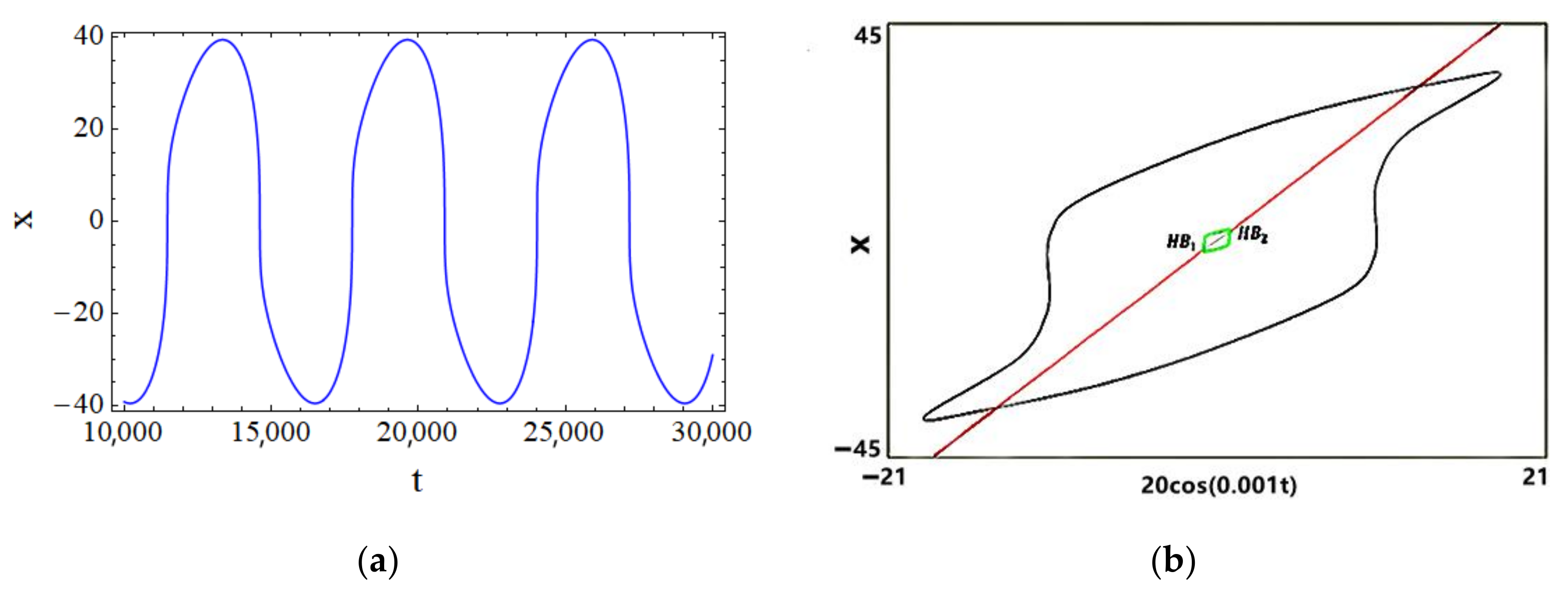
4.4. The Mode of
When
continues to increase to
, the time history diagram and the superposition diagram of the system are drawn, as shown in
Figure 8. From
Figure 8a, another new trajectory emerges. At this time, the system trajectory is still affected by the limit cycle attractor and the stable equilibrium attractor, and the system has the tendency to move away from and close to the attractor. The spiking state completely disappears, and the system only presents the quiescent state mode, as shown in
Figure 8b.
4.5. The Mode of
When
continues to increase to
, the time history diagram and the superposition diagram of the system are drawn, as shown in
Figure 9.
Figure 9b plots the superposition diagram, from which it can be seen that the system trajectory slowly moves around the limit cycle and the equilibrium point. As
weakens, the attractivity of the attractor also weakens, and the influence of periodic excitation becomes more and more significant.
4.6. Summary
To sum up, both fast- and slow-varying processes affect the vibration mode of the system. When is small, the system has two kinds of frequencies and is more affected by the fast-varying process. When gradually increases, increases, and the influence of the slow-varying process is gradually reflected. At this time, the bursting phenomenon will occur. When reaches a certain value, the system is only affected by the slow-varying process and presents a simple periodic vibration mode.
In
Figure 5,
Figure 6,
Figure 7,
Figure 8 and
Figure 9b, we reveal the vibration mode mechanism of (a), and
vibrates in
. The system trajectory encounters different types of attractors in the fast subsystem, resulting in different vibration modes. When
is small, the system trajectory presents the spiking state under the influence of stable limit cycle attractor. As
increases gradually, the system trajectory will be affected by both the limit cycle attractor and stable equilibrium attractor, which shows a "bistable state" bursting situation. Moreover, the spiking state and the quiescent state alternately appear in the same period. Finally, the influence of periodic excitation is increasing, the attraction of the fast subsystem is becoming weaker and weaker, the system appears a single periodic motion, and the trajectory moves around the limit cycle and the equilibrium point.
5. Conclusions
In this paper, the dynamic behavior of the van der Pol-Rayleigh system with the double Hopf bifurcations generated by external excitation is studied by the fast–slow analysis method.
Firstly, the stability and bifurcation behavior of the equilibrium point of the system (2) are analyzed. By analyzing the characteristic equation, we know that the equilibrium point of the system has different properties under different conditions. In addition, the system has no fold bifurcation point, but may have a Hopf bifurcation point. By calculating the Hopf bifurcation’s transversality condition, we find that the Hopf bifurcation theorem holds and a Hopf bifurcation point exists in the system. By calculating the first Lyapunov coefficient, the bifurcation direction and stability of Hopf bifurcation are obtained.
Then, the fast subsystem is simulated numerically and analyzed with or without external excitation. By comparing the time history diagrams with different values, it is found that the parameters have a certain influence on the bursting oscillation of the system.
Finally, the vibration mechanism of the system under different modes is analyzed. The vibration mode of the system is affected by both the fast- and slow-varying processes. The mechanism of different modes vibration of the system is revealed by the transformation phase portrait method, because the system trajectory will encounter different types of attractors in the fast subsystem. When the external excitation amplitude is small, the system trajectory presents the spiking state under the influence of a stable limit cycle attractor. As the external excitation amplitude increases gradually, the system trajectory will be affected by both the limit cycle attractor and stable equilibrium attractor, which shows a “bistable state” bursting situation. When the external excitation amplitude reaches a certain value, the system is only affected by the slow-varying process and presents a simple periodic vibration mode.
Author Contributions
Conceptualization, Y.Q.; methodology, Y.Q.; software, D.Z.; validation, D.Z.; writing—original draft preparation, D.Z.; writing—review and editing, Y.Q. and D.Z. All authors have read and agreed to the published version of the manuscript.
Funding
The reported study was funded by the National Natural Science Foundation of China. (NNSFC) for the research project Nos. 12172333,11572288 and the Natural Science Foundation of Zhejiang through grant no. LY20A020003.
Data Availability Statement
All data, models, and code generated or used during the study are included within the article.
Acknowledgments
The authors gratefully acknowledge the support of the National Natural Science Foundation of China (NNSFC) through grant nos. 12172333 and 11572288 and the Natural Science Foundation of Zhejiang through grant no. LY20A020003.
Conflicts of Interest
The authors declare that there are no conflicts of interest regarding the publication of this paper.
References
- Luo, A.C.J.; Xing, S.Y. Multiple bifurcation trees of period-1 motions to chaos in a periodically forced, time-delayed, hardening Duffing oscillator. Chaos Solitons Fractals 2016, 89, 405–434. [Google Scholar] [CrossRef]
- Luo, A.C.J.; Min, F.H. The chaotic synchronization of a controlled pendulum with a periodically forced, damped Duffing oscillator. Commun. Nonlinear Sci. Numer. Simul. 2011, 16, 4704–4717. [Google Scholar] [CrossRef]
- Jiang, Y.; Shen, Y.J.; Wen, S.F. Super-harmonic and sub-harmonic simultaneous resonance of fractional-order van der Pol oscillator. J. Vib. Eng. 2019, 32, 863–873. [Google Scholar]
- Wu, Z.Q.; Wang, W.B.; Zhang, X.Y. A tri-stable Van der Pol system’s stochastic P-bifurcation circuit experiment. J. Vib. Shock 2018, 37, 111–116. [Google Scholar]
- Wang, Z.X.; Chen, H.B. The saddle case of a nonsmooth Rayleigh–Duffing oscillator. Int. J. Non-Linear Mech. 2021, 129, 103657. [Google Scholar] [CrossRef]
- Zhou, L.Q.; Chen, F.Q. Chaos of the Rayleigh–Duffing oscillator with a non-smooth periodic perturbation and harmonic excitation. Math. Comput. Simul. 2022, 192, 1–18. [Google Scholar] [CrossRef]
- Erlicher, S.; Trovato, A.; Argoul, P. A modified hybrid Van der Pol/Rayleigh model for the lateral pedestrian force on a periodically moving floor. Mech. Syst. Signal Process. 2013, 41, 485–501. [Google Scholar] [CrossRef]
- Tang, J.H.; Li, X.H.; Shen, Y.J. Bursting oscillation and its mechanism of van der Pol-Rayleigh system under periodic excitation. J. Vib. 2019, 32, 1067–1076. [Google Scholar]
- Saha, S.; Gangopadhyay, G.; Ray, D.S. Systematic designing of bi-rhythmic and tri-rhythmic models in families of Van der Pol and Rayleigh oscillators. Commun. Nonlinear Sci. Numer. Simul. 2020, 85, 105234. [Google Scholar] [CrossRef]
- Hasegawa, H. Jarzynski equality in van der Pol and Rayleigh oscillators. Phys. Rev. E 2011, 84, 061112. [Google Scholar] [CrossRef] [PubMed] [Green Version]
- Jerzy, W. Regular and Chaotic Vibrations of Van Der Pol and Rayleigh Oscillators Driven by Parametric Excitation. Procedia IUTAM 2012, 5, 78–87. [Google Scholar]
- Veskos, P.; Demiris, Y. Experimental comparison of the van der Pol and Rayleigh nonlinear oscillators for a robotic swinging task. In Proceedings of the AISB 2006 Conference, Adaptation in Artificial and Biological Systems, Bistrol, UK, 3–6 April 2006; Volume 1, pp. 197–202. [Google Scholar]
- Chen, H.B.; Tang, Y.L.; Xiao, D.M. Global dynamics of hybrid van der Pol-Rayleigh oscillators. Phys. D Nonlinear Phenom. 2021, 428, 133021. [Google Scholar] [CrossRef]
- Bartkowiak, R.; Woernle, C. The Rayleigh–van der Pol oscillator on linear multibody systems. Int. J. Non-Linear Mech. 2018, 102, 82–91. [Google Scholar] [CrossRef]
- Chen, Z.; Chen, S.Y.; Ye, X.J. A Study on a Mechanism of Lateral Pedestrian-Footbridge Interaction. Appl. Sci. 2019, 9, 5257. [Google Scholar] [CrossRef] [Green Version]
- Rinzel, J. Bursting oscillations in an excitable membrane model. Ordinary Part. Differ. Equ. 1985, 1151, 304–316. [Google Scholar]
- Han, X.J.; Jiang, B.; Bi, Q.S. Symmetric bursting of focus–focus type in the controlled Lorenz system with two time scales. Phys. Lett. A 2009, 373, 3643–3649. [Google Scholar] [CrossRef]
- Qu, R.; Wang, Y.; Wu, G.Q.; Zhang, Z.D.; Bi, Q.S. Bursting Oscillations and the Mechanism with Sliding Bifurcations in a Filippov Dynamical System. Int. J. Bifurc. Chaos 2018, 28, 1850146. [Google Scholar] [CrossRef]
- Bao, B.C.; Wu, P.Y.; Bao, H.; Wu, H.G.; Zhang, X.; Chen, M. Symmetric periodic bursting behavior and bifurcation mechanism in a third-order memristive diode bridge-based oscillator. Chaos Solitons Fractals 2018, 109, 146–153. [Google Scholar] [CrossRef]
- Zhou, C.Y.; Li, Z.J.; Xie, F.; Ma, M.L.; Zhang, Y. Bursting oscillations in Sprott B system with multi-frequency slow excitations: Two novel “Hopf/Hopf”-hysteresis-induced bursting and complex AMB rhythms. Nonlinear Dyn. 2019, 97, 2799–2811. [Google Scholar] [CrossRef]
- Li, Z.J.; Fang, S.Y.; Ma, M.L.; Wang, M.J. Bursting Oscillations and Experimental Verification of a Rucklidge System. Int. J. Bifurc. Chaos 2021, 31, 2130023. [Google Scholar] [CrossRef]
- Kuznetsov, Y.A. Elements of Applied Bifurcation Theory, 3rd ed.; Springer: New York, NY, USA, 2004. [Google Scholar]
Figure 1.
Bifurcation diagram of the system (2) with respect to
when , , , , , .
Figure 1.
Bifurcation diagram of the system (2) with respect to
when , , , , , .
Figure 2.
The vibration models of the original MHVDR system when : (a) the phase plane portrait when ; (b) the time history diagram when ; (c) the phase plane portrait when ; (d) the time history diagram when .
Figure 2.
The vibration models of the original MHVDR system when : (a) the phase plane portrait when ; (b) the time history diagram when ; (c) the phase plane portrait when ; (d) the time history diagram when .
Figure 3.
The time history diagram of the MHVDR system under slow external excitation: (a) , , ; (b) , , ; (c) , , ; (d) , , .
Figure 3.
The time history diagram of the MHVDR system under slow external excitation: (a) , , ; (b) , , ; (c) , , ; (d) , , .
Figure 4.
The phase plane portrait of the MHVDR system under slow external excitation: (a) , , ; (b) , , ; (c) , , ; (d) , , .
Figure 4.
The phase plane portrait of the MHVDR system under slow external excitation: (a) , , ; (b) , , ; (c) , , ; (d) , , .
Figure 5.
The time history diagram and the superposition diagram of the system when : (a) the time history diagram; (b) the superposition diagram.
Figure 5.
The time history diagram and the superposition diagram of the system when : (a) the time history diagram; (b) the superposition diagram.
Figure 6.
The time history diagram and the superposition diagram of the system when : (a) the time history diagram; (b) the superposition diagram.
Figure 6.
The time history diagram and the superposition diagram of the system when : (a) the time history diagram; (b) the superposition diagram.
Figure 7.
The time history diagram and the superposition diagram of the system when : (a) the time history diagram; (b) the superposition diagram.
Figure 7.
The time history diagram and the superposition diagram of the system when : (a) the time history diagram; (b) the superposition diagram.
Figure 8.
The time history diagram and the superposition diagram of the system when : (a) the time history diagram; (b) the superposition diagram.
Figure 8.
The time history diagram and the superposition diagram of the system when : (a) the time history diagram; (b) the superposition diagram.
Figure 9.
The time history diagram and the superposition diagram of the system when : (a) the time history diagram; (b) the superposition diagram.
Figure 9.
The time history diagram and the superposition diagram of the system when : (a) the time history diagram; (b) the superposition diagram.
| Publisher’s Note: MDPI stays neutral with regard to jurisdictional claims in published maps and institutional affiliations. |
© 2021 by the authors. Licensee MDPI, Basel, Switzerland. This article is an open access article distributed under the terms and conditions of the Creative Commons Attribution (CC BY) license (https://creativecommons.org/licenses/by/4.0/).


