A Novel Plain-Text Related Image Encryption Algorithm Based on LB Compound Chaotic Map

Abstract

Chaos systems have been widely used in image encryption algorithms. In this article, we introduce an LB (Logistic-Baker) compound chaotic map that can greatly improve the complexity of original Logistic map and Baker map, as well as the generated sequences have pseudo-randomness. Furthermore, based on the LB compound chaotic map, an image encryption algorithm is proposed. To resist the differential attack, and enhance the sensitivity of plain-text, the parameters of this algorithm are plain-text related. In this algorithm, the compound chaotic function is influenced by the plain-text image; thus, the specific form of this chaotic map, and its dynamics will be different when encrypting different images. Numerical experiment results indicate that the effect of this novel plain-text related image encryption scheme is excellent, as well as can be competitive with other corresponding algorithms.

1. Introduction

1.1. Background

The security of digital image has achieved wide attention from both scholars and industries [1,2,3,4]. At first, scholars used traditional text encryption algorithms, such as DES, AES, RSA, and so on, to encrypt the images. However, such image encryption algorithms have some inherent weaknesses, including uneven energy distribution, strong correlation between adjacent pixels, and high data redundancy [5,6,7,8]. All these defects make the traditional encryption algorithms not suitable to encrypt digital images.

Today, a kind of novel image encryption algorithm has been introduced, which is called chaos-based image encryption. Chaos is a complex physical phenomena, which can be represented in many dynamical systems. Chaotic systems have many advantage characteristics, such as sensitivity for initial conditions, rapid decay of the correlations and pseudo-randomness, etc. All these characteristics make chaotic systems quite suitable for image encryption.

Among the chaotic image encryption algorithms, the low-dimensional chaotic maps are often used in many studies [9,10,11,12]. However, the security of these chaotic maps are quite low due to their simple structures; furthermore, they will suffer the threaten from phase space reconstruction technology. Ref. [13] proves that the phase space reconstruction technology is effective for most of the low-dimensional chaotic maps. To improve the complexity of image encryption algorithms, some studies use high-dimensional chaotic systems as the random sources, and even hyper-chaotic systems with very high dimensions are used [14,15,16,17,18,19,20]. Using high-dimensional chaotic systems can certainly improve the complexity of encryption algorithms. However, different from the low-dimensional chaotic system, the high-dimensional chaotic system has more parameters and initial values [21], which means that the high-dimensional chaotic system needs more calculations when calculating the sequence of the same dimension [22]. In other words, these systems always require high cost to implement, which is not suitable for practical uses. Based on the above two conditions, a more appropriate thinking is to use improved low-dimensional chaotic maps in image encryption. On one side, the low-dimensional chaotic maps can ensure the speed of encryption and are much easy to implement. On the other side, some improvement methods can effectively improve the complexity of low-dimensional chaotic maps and then enhance the security of the encryption algorithms [21,23,24,25,26,27].

Motivated by this, in this paper, we first propose a new chaotic map by compounding 1-D Logistic map and 2-D Baker map. Numerical experiments show that the compound chaotic map greatly improve the complexity of original maps. The results of NIST statistical test evaluate the randomness of the generated sequences by this compound chaotic map. Furthermore, after constructing this compound chaotic map, we propose a novel image encryption algorithm based on this map. It is acknowledged that, if the image encryption algorithm is independent to plain-text image, then, it will easily suffer the differential attack (chosen-plain-text attack), which leads to a high security risk. Therefore, some encryption algorithms try to put some of the plain-text information into the encryption process to make it plain-text related, such as refs. [21,24]. However, the parameters of chaotic maps used in these studies are independent of the image information of plain-text images, which means that the parameters of these chaotic maps may be invariant when encrypting different images. In other words, the specific form of these maps does not change; only the initial values do. Thus, in this paper, a novel plain-text related image encryption algorithm is proposed. In this encryption scheme, the value of parameters of this chaotic map are related to the plain-text image. It means that the specific form of this chaotic map will change as the encrypted image changes, and this change is image-related. In the numerical tests, we use four standard common images (“Lena”, “Cameraman”, “Horse”, and “Granules”) to prove that the proposed algorithm is practical for different images.

In addition, we use numerical tests and analysis to evaluate the security performance of this encryption algorithm. The key space analysis is used to estimate the secret key space of this algorithm; the histogram analysis is used to test the distribution of pixel values; the key sensitivity analysis is used to test the sensitivity of secret key; the correlation analysis is used to test the correlation between two neighboring pixels; the information entropy analysis is used to estimate the uncertainty and randomness of images. To measure the ability to resist differential attack of this encryption algorithm, two statistical indicators are used, named number of pixels change rate (NPCR) and unified average changing intensity (UACI). When the bit stream is transmitting on the internet, the occurrence of data loss and data interference by noise is inevitable [28]; in fact, the methods in which noise signals were applied are known from the time of WWII, when they were applied to encrypt the correspondence of intelligence services. Thus, the robustness analysis of this encryption algorithm is necessary. Finally, the computational complexity analysis is used to measure the speed of encryption algorithm.

1.2. Related Works

1.2.1. Low Dimensional Chaotic Maps-Based Image Encryption Algorithms

A novel piecewise linear chaotic map (PWLCM)-based chaotic image encryption algorithm provided in ref. [9]. In this scheme, the hash function is used as an initial conditions generator for PWLCM. Ref. [10] provides a new 1-D chaotic map, and bifurcation analysis and Lyapunov exponent analysis are used to demonstrate its chaos performance. In addition, to declare its practicability, a simple but efficient image encryption scheme is utilized. In ref. [11], to strengthen the connection between the encryption algorithm and the plain-text image, a Chebyshev function is introduced. The key stream used to encrypt the images is generated by this function. In ref. [12], the 1-D chaotic tent map is used to design a novel image encryption scheme, with efficient and secure performances, etc. Generally speaking, low-dimensional chaotic maps have many great features, such as easy to be realized and having a rapid computing speed.

1.2.2. High Dimensional Chaotic Maps-Based Image Encryption Algorithms

In ref. [14], to improve the security of traditional image encryption algorithms, a rewriting scheme is added. Moreover, a two-dimensional modulation chaotic map basic of Sine map and Logistic map is introduced. Ref. [15] proposed an improved chaotic system based on 3-D Lorenz chaotic map and 4-D Rossler chaotic map. In addition, a novel DNA coding-based color image encryption algorithm is utilized. In ref. [16], an image encryption based on hash function and cat map is provided. In this scheme, the hash function is used to generate the set of keys used as initial values of this encryption algorithm. In addition, a new matrix magic transformation (MMT) algorithm is also proposed. Ref. [17] proposed a multidimensional chaotic image encryption algorithm based on improved 3-D Lorenz system. The improved system become a four-dimensional hyperchaotic system. Ref. [18] introduced an image encryption scheme, in which a 6-D hyperchaotic system and a Logistic-Sine compound chaotic map are utilized. In ref. [19], a 4-D hyperchaotic system and a 1-D Logistic-Tent map are applied to generate chaotic sequence. In addition, a color image encryption based on compressive sensing is proposed. Moreover, a DNA coding and three chaotic maps-based image encryption algorithm is investigated in ref. [20]. The simulation results shows that this scheme has high security, etc.

1.2.3. Improved Low Dimensional Chaotic Maps-Based Image Encryption Algorithms

Ref. [21] proposed a novel image encryption algorithm based on coupled Baker map and Logistic map. The Baker map is used to control the initial values of the Logistic map, which makes the generated Logistic sequence become non-stationary. Ref. [23] described a modification of the Logistic map which helps it to achieve greater robustness against phase space reconstruction attacks. Furthermore, an image encryption algorithm based on this modified map is proposed. Ref. [24] proposed a varying parameters Logistic map-based image encryption scheme. Ref. [25] proposed a two-dimensional modular chaotic system that can improve the performance of chaos, and various tests proved that this model can improve thedynamical complexity. Ref. [26] proposed a novel pseudorandom generator based on improved one-dimensional chaotic map amplifier (1-DCMA) to encrypt the plain-text images, etc. Compounding multiple chaotic maps is another kind of effective method to improving the complexity of chaotic maps [29,30,31,32]. Ref. [29] proposed a compound chaotic map based on even-symmetric chaotic maps and a skew Tent map, which is applied to image encryption. Ref. [30] proposed an image encryption algorithm based on Lu and Logistic compound system. In ref. [31], a compound Tent-Logistic chaotic system is presented. This compound system has good randomness and large key space. In ref. [32], a two-dimensional Logistic-Tent modular map was proposed. Based on this chaotic map, a cross-plain image encryption scheme is used to encrypted the color image, etc.

The rest of this paper is shown as follows. In Section 2, a novel compound chaotic map is proposed, and several complexity and randomness analysis are presented. In Section 3, a novel plain-text related image encryption algorithm is provided. Numerical experiments of the security analysis of this encryption algorithm are presented in Section 4. Finally, Section 5 sums up this whole paper.

2. The Proposed Compound Chaotic Map and Its Performance

2.1. A Novel LB Compound Chaotic Map

Among all chaotic maps, Logistic map can be said as the most simple and popular map in data encryption [21,33,34]. The mathematical model of the Logistic map can be written as:

$$x_{i+1}=f\left(x_i\right)=a{x}_i \left(1-x_i\right).$$

(1)

Here, f is the chaotic iteration function, x_i is the state variable, and a is the bifurcation coefficient. The function f become chaotic once the coefficient a locates in the interval (3.5699, 4]. The variable x_i is bounded in the interval (0, 1). Once giving an initial condition x₀, under the control of iterative function f, a sequence {x_i} will be generated. For an ideal chaotic map, the generated sequence should have a high complexity, with good randomness.

The complexity analysis of logistic sequences is depicted in Figure 1a,b. Figure 1a shows the approximate entropy (ApEn) of logistic sequence with different parameters. ApEn was firstly proposed by Pincus in ref. [35], which measures the probability of the new pattern generated in the sequences with the embedding dimension grows. The larger the probability means more complex of sequence. For a series {v(i), i = 1, 2, …, N}, recombining this sequence: U_i = {v(i), v(i + 1), …, v(i + m − 1)}, i = 1, 2, …, n, n = N − m + 1, we can get a m-dimensional vector U_i. Next, calculate the distance between U_i and U_j as:

$$L_{ij}=\max \left|v\left(i+j\right)-v\left(j+k\right)\right|,k=0, 1, \dots ,m-1 .$$

(2)

Set a threshold b = 0.2~0.3, and give a number X that satisfies the standard L_ij ≤ b × SD, in which SD is a standard value of sequence. Then, we have C_i^m (b) = X/(N − m), and

$${\omega }^m\left(b\right) = \frac{1}{N-m+1}{\sum }_{i=1}^{N-m+1}ln{C}_i^m\left(b\right) .$$

(3)

Finally, the approximate entropy can be calculated as ω^m − ω^m+1. From Figure 1a, we can find that, with the growth of parameters, the ApEn will gradually increase on the whole. However, in some intervals, the ApEn will have a quick decline, which reflects to the period windows of control coefficient of Logistic map (period windows means the non-chaotic region in the chaotic parameter interval). The Logistic map has the largest ApEn when a = 4, which is about 0.656483.

Another sequence complexity measure is called permutation entropy (PE), which was introduced by Bandt and Pompe in ref. [36]. PE uses Shannon’s entropy to measure the probabilities of different order types of consecutive values in the sequences. In this test, we choose the ordinal pattern length L = 6, and the embedding delay D = 2 as suggested in ref. [36]. For a series {v(i), i = 1, 2, …, N}, we need to know as possible order types of n different numbers (i.e., n! permutations μ of order n). For each number μ, we calculate the relative frequency (# means number):

$$F\left(\mu \right) = \frac{\#\left\{t\left|t\le N-n,\left(v_{t+1}, \dots ,v_{t+n}\right) hastype \mu \right.\right\}}{N-n+1} .$$

(4)

To make the F(μ) more exact, assume the N → ∞, and {v(i), i = 1, 2, …}. This limit exists with probability 1 when the underlying stochastic process satisfies the condition: for k ≤ n, the probability for v(t) < v(t + k) should not be related to t. Thus, the permutation entropy of order n ≥ 2 can be calculated as:

$$H\left(n\right) = -\sum F\left(\mu \right)logF\left(\mu \right) ,$$

(5)

where the sum runs over all n! permutations p of order n.

The test results are shown in Figure 1b. As Figure 1b shows, with the growth of parameters, the PE will increase gradually on the whole, which is similar to the results of ApEn analysis. When the coefficient a fall into the period window, the PE will quickly decline, as well. PE gets its maximum value 0.947877 when a = 4.

Besides Logistic map, Baker map has good ergodicity and distribution characteristics, which is also widely used in image encryption today [37,38,39]. Its mathematical model can be described as follows.

$$\left(x_{i+1},y_{i+1}\right) = \left\{\begin{array}{cc}\left(x_i/p,p{y}_i\right)\hfill & 0\le x_i\le p\\ \left(\left(x_i-p\right)/\left(1-p\right),\left(1-p\right)y_i+p\right)\hfill & p\le x_i\le 1\end{array}\right.,$$

(6)

where p ∈ (0, 1) is the control parameter, and (x_i, y_i) is the 2D state variable. The output sequence (x_i, y_i) has good ergodicity in the phase space [0, 1] × [0, 1]. When p = 0.5, it will become the standard Baker map. It should be noted that, when p = 0.5, the standard Baker map will be seriously affected by computer precision, and the output sequence will quickly fall into a cycle. Therefore, we will not choose p = 0.5 in our test.

The ApEn and PE analysis of Baker sequences are depicted in Figure 2. In this test, the x-dimensional variable is used as the test data. For y-dimensional variable, the results are similar, which we omitted here to avoid redundancy. From Figure 2a,b, we can conclude that the complexity (both ApEn and PE) will monotonically increase with the growth of parameter p. The complexity of the Baker map is symmetrical when p > 0.5 and p < 0.5. The Baker map get its largest complexity when p is close to 0.5, which is about 0.691743 for ApEn, and 0.933645 for PE.

As the test results show above, the complexity of these two chaotic maps are quite low, and their output sequences cannot be regarded to have high security level. Encryption algorithms directly based on these two chaotic maps will suffer security risks. Therefore, in order to improve its complexity, a novel compound LB chaotic map is provided here, whose mathematical formula can be directly written as follows.

$$\left(x_{i+1},y_{i+1}\right) = \left\{\begin{array}{cc}\left(a{x}_i\left(1-x_i\right)/p,p{y}_i\right)\hfill & 0\le a{x}_i\left(1-x_i\right)\le p\\ \left(\left(a{x}_i\left(1-x_i\right)-p\right)/\left(1-p\right),\left(1-p\right)y_i+p\right)\hfill & p\le a{x}_i\left(1-x_i\right)\le 1\end{array}\right..$$

(7)

As Equation (7) shows, the LB compound chaotic map has two control parameters, a and p. In this compound chaotic map, we use Logistic map to compound the x-dimensional variable of Baker map. Similarity, the y-dimensional variable can also be compounded, whose mathematical model can be described as

$$\left(x_{i+1},y_{i+1}\right) = \left\{\begin{array}{cc}\left(x_i/p,pa{x}_i{\left(1-x_i\right)}_i\right)\hfill & 0\le x_i\le p\\ \left(\left(x_i-p\right)/\left(1-p\right),\left(1-p\right)a{x}_i\left(1-x_i\right)+p\right)\hfill & p\le x_i\le 1\end{array}\right..$$

(8)

These two compound chaotic maps have no essential differences. Equation (7) improves the complexity of x-dimensional variable, while Equation (8) improves the complexity of y-dimensional variable. In the above tests, we use x-dimensional variable as the test data. Thus, we use the compound map in Equation (7) throughout the whole paper.

2.2. The Performances of the LB Compound Chaotic Map

Next, we will take some numerical experiments to analyze the characteristics of the LB compound chaotic map, including trajectories, bifurcation diagram, auto-correlation function, complexity and NIST statistical tests. In these tests, the initial value and parameters are set as x₀ = 0.1260, y₀ = 0.3259, a = 4, p = 0.499, unless otherwise stated. The x-dimensional variable is used in these tests.

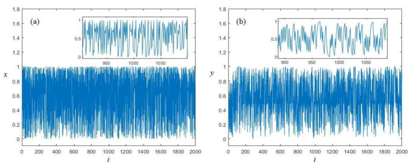
2.2.1. Sequence Generation Algorithm

Trajectory gives an intuitive expression of the dynamics of the LB compound chaotic map. Both x and y dimensional variables are plotted in Figure 3. From Figure 3, we can see that the generated sequences are random-like, without any obvious structures or cycles. Furthermore, the value of both x and y dimensional variables can cover the whole interval (0, 1), which indicates that this LB compound chaotic map has a good ergodicity.

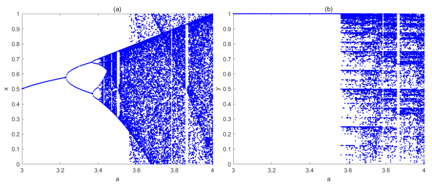
2.2.2. Bifurcation Diagram

Bifurcation diagram reflects the relationship between chaotic characteristics and control parameters. For different parameter p ∈ (0, 1), the map will always be chaotic. Here, we just reveal the bifurcation diagram of control parameter a, which is depicted in Figure 4. As Figure 4 shows, the x-dimensional variable of the LB compound map comes to be chaotic at about a > 3.45, and the y-dimensional variable of the LB compound map comes to be chaotic at about a > 3.55. Since parameter a comes from Logistic map, thus, we compare this result with the bifurcation diagram of logistic chaotic map. As we know, Logistic map will come to be chaotic since a > 3.5699, which implies that this LB compound chaotic map has a larger chaotic parameter region. Furthermore, the output of original Logistic map will cover the whole interval (0, 1) only when a = 4, while, in this LB compound map, the output will cover the whole interval (0, 1) since a > 3.57, which implies that this compound map has a better ergodicity. Similar with Logistic map, this compound chaotic map also has several period windows, which should be avoided in practical uses.

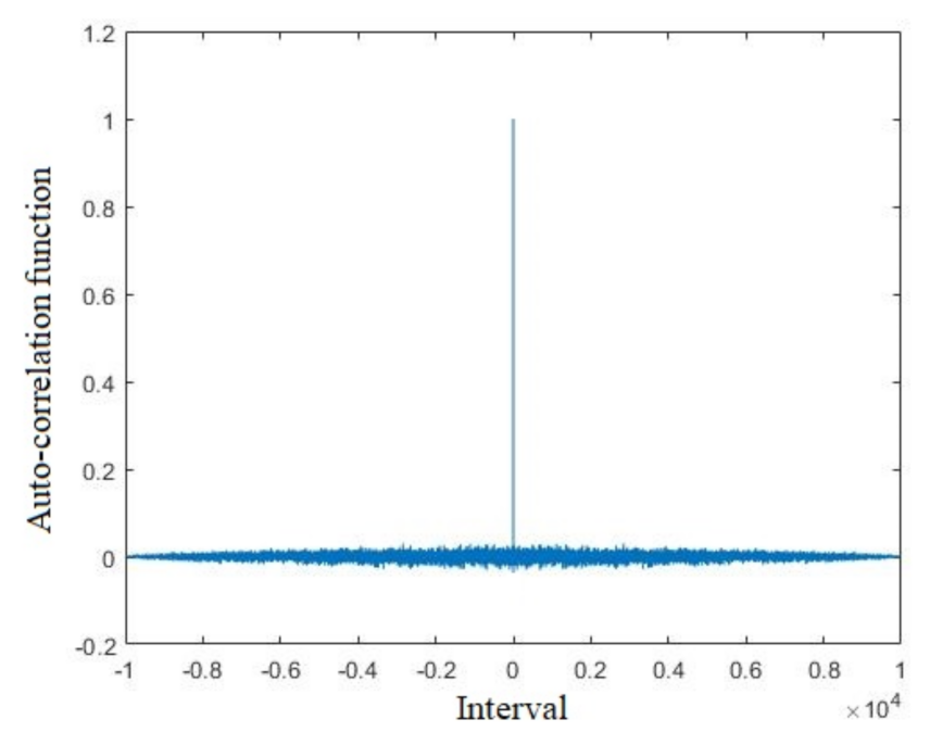
2.2.3. Auto-Correlation Analysis

Auto-correlation function reflects the relationship between the state variable at one time and the state variables at other times. The mathematical model of auto-correlation function can be shown as:

$$\begin{gathered} r_k=\frac{{\sum }_{t=1}^{N-k}\left(x_t-\overline{x}\right)\left(x_{t+k}-\overline{x}\right)}{{\sum }_{t=1}^N{\left(x_t-\overline{x}\right)}^2} \\ -1\le r_k=\frac{r_k}{r_0}\le 1 , \end{gathered}$$

(9)

where x_t (t = 0, 1, …, N) is state variable sequence, and k is a spacing coefficient. When k = 0, the coefficient r_k = 1 means the relationship between the state variable and itself. For an ideal pseudo-random sequence, its auto-correlation function should be delta function. The auto-correlation analysis of the LB compound chaotic map is shown in Figure 5. From Figure 5, the auto-correlation function is extremely close to the ideal model, which means that the generated sequence of the LB compound chaotic map can be regarded as a pseudo-random sequence in this sense.

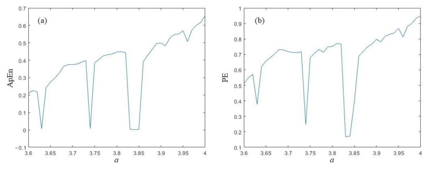
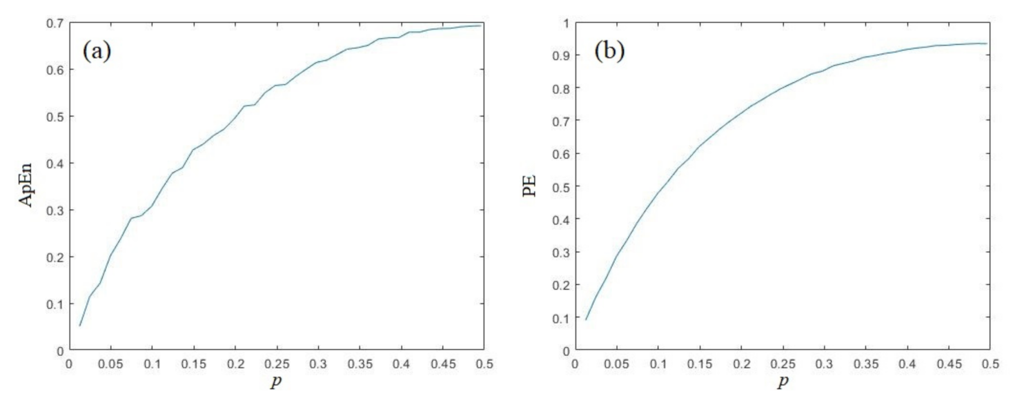
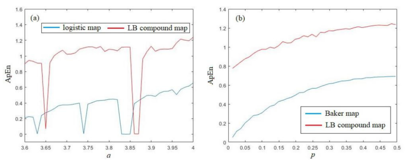
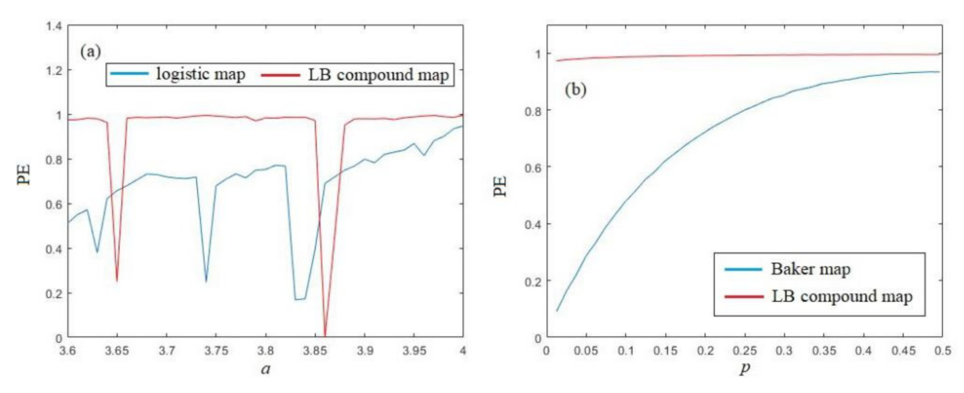
2.2.4. ApEn and PE Analysis

The main purpose of this LB compound chaotic map is to improve the chaotic behavior of original chaotic maps. Here, we also test the ApEn and PE of the compound chaotic map, and compare them with the complexity of original chaotic maps. The ApEn analysis and comparison with the Logistic map and Baker map are provided in Figure 6a,b, respectively. From Figure 6a, we have that the ApEn of the LB compound chaotic map is larger than the original Logistic map for almost all different parameter a, except when a falls into the period windows. Furthermore, we can also find that the ApEn of the LB compound chaotic map is quite stable for different parameter a (without period windows), while the ApEn of the Logistic map when a < 3.8 is obviously smaller than the values when a is close to 4. This is an advantage that the LB compound chaotic map can maintain at a high complexity level for different parameters, while the complexity of original Logistic map is rather low when the parameters are smaller than 3.8, although the map is chaotic under these parameters. From Figure 6b, we can also find that the ApEn of the LB compound chaotic map is larger than the original Baker map for all different parameters p.

Similar results can be obtained from PE analysis, shown in Figure 7a,b. Figure 7a shows that the PE of the LB compound chaotic map is larger than PE of the Logistic map for almost all parameters, except the period windows. From Figure 7b, we can also find that the PE of the LB compound chaotic map is larger than PE of the original Baker map for all parameters. Furthermore, both results show that the PE of the LB compound chaotic map is extremely close to the ideal value 1, which implies that the LB compound chaotic map has an ideal complexity level.

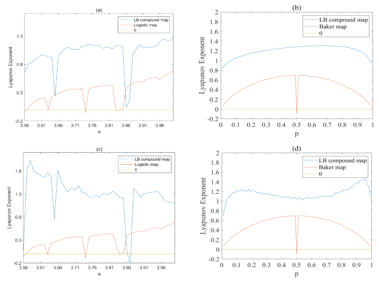
2.2.5. Lyapunov Exponent

Lyapunov exponent (LE) is used to indicate the divergence rate of two trajectories, which is a key index for chaotic system. In this paper, the Wolf algorithm [40] is used to calculate the LE of generated sequences. If the largest LE of a system is larger than zero, this system can be regarded as chaotic. The LE value of x and y dimensional variables of the LB compound map with different parameters a and p are shown in Figure 8a–d, respectively. As Figure 8a,c show, the LE values of x and y dimensional variables of the LB compound map are larger than zero with different parameter a, although the LE will decrease rapidly when parameter a falls into the periodic period. Furthermore, the LE value will have a significant improvement when comparing with the original Logistic map. Similar results can be obtained for the parameter p. As Figure 8b,d shows, the LE values are all great than zero and larger than the LE of original Baker map, as well. The results proves that the LB compound chaotic map has greatly improved the chaotic performances of original chaotic maps.

2.2.6. NIST Statistical Tests

Among all statistical tests suites, NIST statistical test suite has been regarded as current industry norm for randomness testing [41]. NIST statistical test suite contains 16 independent statistical tests to test the randomness of binary sequences. In NIST, the significance level is set to be 0.01. A sequence is regarded to pass the statistical test when p-value ≥ 0.01. To test the randomness of the sequences generated by the LB compound chaotic map, here, we have generated 500 different sequences by 500 randomly chosen initial conditions. Since NIST statistical test suite is only used for binary sequences, thus, before the test, we use the following binarization method:

$$b\left(x_i\right) = floor\left(x_i\times {10}^6\right) mod 256.$$

(10)

By using Equation (10), after 125,000 times of chaotic iterations, the 10⁶ bits length binary sequence can be generated. The passing ratio of each test and the mean value of p-values are shown in

Table 1. NIST test results of the LB compound chaotic map.

Test Index	Passing Ratio	p-Value	Results
Approximate entropy	99.2%	0.765182	Success
Block frequency	99.6%	0.768090	Success
Cumulative sums	99.6%	0.853257	Success
FFT	99.8%	0.876031	Success
Frequency	99.6%	0.564615	Success
Linear complexity	99.8%	0.774610	Success
Random excursions	99.6%	0.563249	Success
Random excursions variant	99.6%	0.359811	Success
Longest runs of ones	99.4%	0.577500	Success
Overlapping template of all ones	99.6%	0.769284	Success
Rank	99.8%	0.266723	Success
Runs	99.6%	0.131128	Success
Serial	99.4%	0.320054	Success
Universal statistical	99.6%	0.621337	Success
Lempel-Ziv Compression Test	99.8%	0.423651	Success

. From Table 1, we can have the conclusion that the sequences generated by the LB compound chaotic map have good statistical properties, and they can be regarded as random sequences.

3. A Novel Plain-Text Related Image Encryption Algorithm

3.1. A Plain-Text Related LB Compound Chaotic Map

Based on the ideal properties of the LB compound chaotic map Equation (7), in this section, we propose an image encryption algorithm based on this map. To resist the differential attack, the encryption process should be related to the plain-text image. Since using some information of plain-text image to change the initial value of chaotic map will not affect the chaotic system itself, the chaotic map will remain the same when encrypting different images. Thus, here, we introduce the information of image to the control parameter of chaotic map, whose mathematical model can be described as

$$\left(x_{i+1},y_{i+1}\right) = \left\{\begin{array}{cc}\left(a{x}_i\left(1-x_i\right)/h\left(p,A\right),h\left(p,A\right)y_i\right)\hfill & 0<a{x}_i\left(1-x_i\right)\le h\left(p,A\right)\\ \left(\begin{array}{c}(\left(a{x}_i\left(1-x_i\right)-h\left(p,A\right)\right)/\left(1-h\left(p,A\right)\right),\\ \left(1-h\left(p,A\right)\right)y_i+h\left(p,A\right))\end{array}\right)\hfill & h\left(p,A\right)<a{x}_i\left(1-x_i\right)\le 1\end{array}\right.,$$

(11)

where h(p, A) is defined as

$$h\left(p,A\right) = \left(p+mean\left(A\right)/255\right) mod 1.$$

(12)

Here, mean(A) denotes the mean value of all pixel values of image A.

As Equation (11) shows, the plain-text image information is used to control the parameter p. When encrypting different images, the parameter of the LB compound chaotic map will be different, which makes the chaotic map have different dynamics.

Remark 1.

Using plain-text image information to control the parameter a is not recommended here. From the analysis above, we have that the complexity of the LB compound chaotic map is significantly influenced by parameter a, especially the existence of periodic window. Using plain-text image information to control the parameter a may lead to a low complexity of chaotic map, which affects the encryption performances.

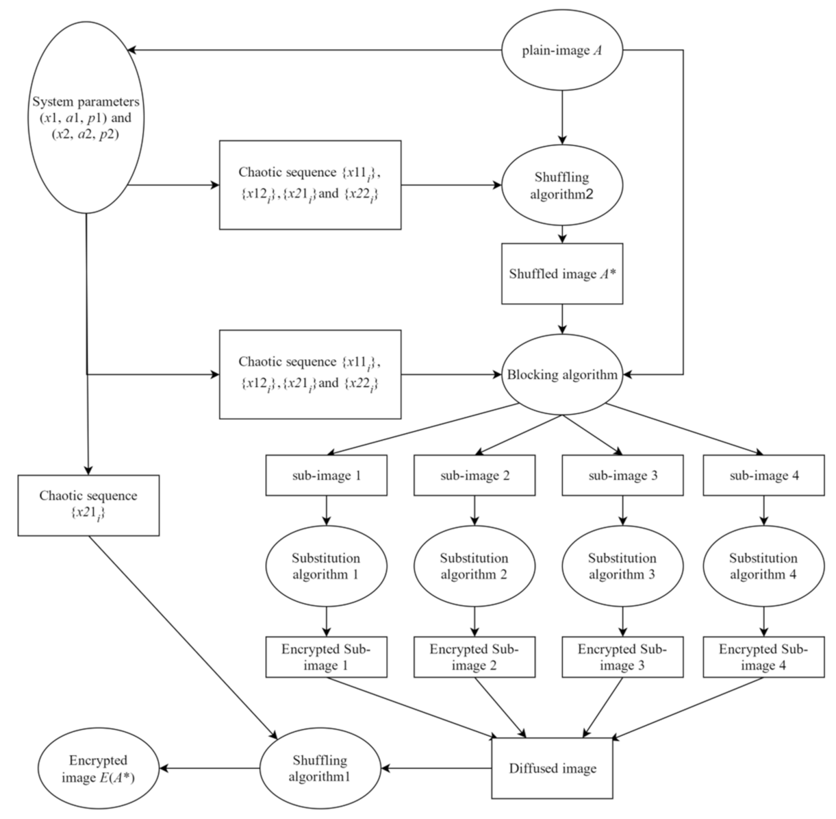
3.2. A Novel Plain-Text Related Image Encryption Algorithm

The proposed plain-text related image encryption algorithm consists of two parts: shuffling algorithm and substitute algorithm.

3.2.1. Shuffling Algorithm 1

As in the PE analysis above, the PE of the LB compound chaotic map is quite close to the ideal value. This result implies that the size order in the generated chaotic sequence is pseudo-random. Therefore, we just shuffle the image according to the size order of the generated chaotic sequence.

Assume A to be the plain-text image with size M × N, its pixel matrix be (A_ij), 1 ≤ i ≤ M, 1 ≤ j ≤ N. {x_i} is the generated sequence with length MN by Equation (11). Define the following order function:

$$order\left(x_p\right) = k,$$

(13)

if x_p is the k-th smallest number in sequence {x_i}, p < MN. Scanning the plain-text image progressively, we can get a pixel sequence {A_q} with length MN. Then, we do the following shuffling:

$$A_i^{*}\leftarrow A_p, order\left(x_p\right) = i, 1\le i\le MN,$$

(14)

where A* is the pixel sequence after shuffling. Equation (14) means that, if x_p is the i-th smallest number in sequence {x_i}, then, we put the pixel value A_p to the i-th value of {A*}. Finally, scan the {A*} into a M × N matrix. Obviously, this shuffling algorithm is completely determined by the size order of the generated chaotic sequence {x_i}. A simple example is given for a more intuitive description of this algorithm.

Example 1.

Assume A be the plain-text image with size 3 × 3, whose pixel matrix can be written as

$$A=\left(\begin{array}{ccc}52& 69& 241\\ 13& 96& 152\\ 7& 19& 183\end{array}\right).$$

(15)

The mean value of all pixel values of A is 92.4444. Setting x₀ = 0.1260, y₀ = 0.3259, a = 4, p = 0.499, according to Equations (11) and (12), we can generate the 3 × 3 length chaotic sequence {x_i} = {0.1260, 0.8828, 0.8296, 0.1325, 0.9212, 0.5817, 0.9468, 0.4040, 0.9265}. Scanning the plain-text image progressively, we can get the pixel sequence {A_q} = {52, 69, 241, 13, 96, 152, 7, 19, 183}. In the sequence {x_i}, we can easily find that x₁ = 0.1260 is the smallest value; thus, according to Equation (14), we have A*₁ = A₁ = 52; Similarly, x₄ = 0.1325 is the 2nd smallest value in {x_i}; thus, we have A*₂ = A₄ = 13; …; x₇ = 0.9486 is the biggest value in {x_i}; thus, we have A*₉ = A₇ = 7. The pixel sequence {A*} after shuffling is {13, 96, 52, 7, 152, 69, 19, 183, 241}. Scanning the sequence {A*} into a 3 × 3 matrix, we can get the image A* after shuffling.

$$A^{*}=\left(\begin{array}{ccc}52& 13& 19\\ 152& 241& 69\\ 96& 183& 7\end{array}\right).$$

(16)

3.2.2. Shuffling Algorithm 2

Different from the shuffling algorithm 1, another shuffling algorithm is proposed, which not only changes the value of pixels but also the position of pixels. The detailed steps are described below.

Assume A be the plain-text image with size M × N. Firstly, scan the image matrix A progressively from left to right to obtain a pixel sequence {P1} with length MN. Secondly, convert the values in sequence {P1} into 8-bit binary numbers and get a sequence {P2}. Thirdly, divide each element of sequence {P2} from left to right into four sub-elements, and each sub-element is a 2-bit binary number. Then, we can get four sequences called {P2a_i}, {P2b_i}, {P2c_i}, and {P2d_i}. Fourthly, use four chaotic sequences to shuffle these four sequences by using the shuffling algorithm 1, respectively. Finally, splice four 2-bit binary elements P2a_i, P2b_i, P2b_i, and P2b_i into one 8-bit binary element P3_i and get a sequence {P3}. The range of i is from 1 to MN. Convert P3_i into decimal number to complete this shuffling algorithm.

3.2.3. Substitution Algorithm

To further prove the randomness of the LB compound chaotic map, in this substitution algorithm, only the xor operation is used. Before substitution, we should first divide the image into four blocks.

The blocking method is based on a chaotic indicator. Assume A be the plain-text image with size M × N, and its pixel matrix is (A_ij), 1 ≤ i ≤ M, 1 ≤ j ≤ N. {x1_i} and {x2_i} are the chaotic sequences generated by Equation (11) with length 2MN. Firstly, calculate the chaotic indicator k:

$$k=p+1=b\left(x{1}_{floor\left(mean\left(A\right)\right)mod MN}\right) mod \left(min\left(M,N\right)\right)+1.$$

(17)

Here, b() is the binarization function defined in Equation (10). From Equation (17), we can find that the indicator k is determined by the mean value of all pixel values of image A.

Then, the image can be divided into four sub-images A1, A2, A3, and A4 according to the chaotic indicator k:

$$A1={\left(A\right)}_{k\times k}, A2={\left(A\right)}_{k\times \left(N-k\right)}, A3={\left(A\right)}_{\left(M-k\right)\times k}, A4={\left(A\right)}_{\left(M-k\right)\times \left(N-k\right)}.$$

(18)

Scanning the generated chaotic sequences {x1_i} and {x2_i} progressively, we can get two couples of chaotic matrixes X1, X2 and X3, X4 with size M × N, respectively. For these four blocks, the substitution algorithms are different.

For the sub-images A1, A2, A3, A4, a bit exchange should be done before substitution. Assume the bit position of an 8-bit integer m is numbered as m₀m₁m₂m₃m₄m₅m₆m₇, m₀, m₁, …, m₇ = 0 or 1. Define a group of transposition functions T_abcd which exchange the bit value at position m_a, m_b with the bit value at position m_c, m_d, 0 ≤ a, b, c, d ≤ 7. For example, function T₀₁₆₇ exchange the bit value at position m₀, m₁ with the bit value at position m₆, m₇. Supposing m = 01101110, we have T₀₁₆₇(m) = 10101101.

Sub-image A1: The substitution algorithm is defined as follows:

$$E\left(A{1}_{ij}\right) = T_{0167} \left(A_{ij}\right) \oplus b\left(X{1}_{ij}\right),$$

(19)

where 1 ≤ i, j ≤ k, and ⊕ denotes the bit-xor operation.

Sub-image A2: The substitution algorithm is defined as follows:

$$E\left(A{2}_{ij}\right) = T_{2345} \left(A_{ij}\right) \oplus b\left(X{2}_{ij}\right),$$

(20)

where 1 ≤ i ≤ k, and k + 1 ≤ j ≤ N.

Sub-image A3: The substitution algorithm is defined as follows:

$$E\left(A{3}_{ij}\right) = T_{0145} \left(A_{ij}\right) \oplus b\left(X{3}_{ij}\right),$$

(21)

where k + 1 ≤ i ≤ M, and 1 ≤ j ≤ k.

Sub-image A4: The substitution algorithm is defined as follows:

$$E\left(A{4}_{ij}\right) = T_{2367} \left(A_{ij}\right) \oplus b\left(X{4}_{ij}\right),$$

(22)

where k + 1 ≤ i ≤ M, and k + 1 ≤ j ≤ N.

A simple example is given for an intuitive description.

Example 2.

Assume A be the plain-text image with size 3 × 3, whose pixel matrix is shown in Equation (15). Set x1 = 0.1260, y1 = 0.5678, a1 = 4, p1 = 0.499 and x2 = 0.3265, y2 = 0.4862, a2 = 3.77, p2 = 0.37, according to Equation (11), and the generated chaotic sequences {x1_i} = {0.1260, 0.8828, 0.8296, 0.1325, 0.9212, 0.5817, 0.9468, 0.4040, 0.9265, 0.5461, 0.9830, 0.1340, 0.9300, 0.5219, 0.9962, 0.0307, 0.2382, 0.4528} and {x2_i} = {0.3265, 0.7286, 0.5960, 0.8535, 0.1607, 0.2199, 0.4394, 0.8867, 0.0138, 0.1382, 0.1254, 0.0691, 0.6550, 0.7650, 0.4886, 0.9080, 0.8515, 0.1692}. According to Equation (10), we have

$$\begin{gathered} b\left(X1\right) = \left(\begin{array}{ccc}48& 121& 75\\ 69& 146& 58\\ 192& 25& 252\end{array}\right), b\left(X2\right) = \left(\begin{array}{ccc}96& 195& 192\\ 215& 200& 129\\ 73& 64& 210\end{array}\right), \\ b\left(X3\right) = \left(\begin{array}{ccc}100& 45& 67\\ 18& 219& 200\\ 59& 33& 184\end{array}\right), b\left(X4\right) = \left(\begin{array}{ccc}215& 151& 178\\ 226& 33& 84\\ 187& 168& 247\end{array}\right). \end{gathered}$$

(23)

By mean value of all pixel values of A is 92.4444, thus, according to Equation (17), we have

$$p=b\left(x{1}_{92 mod 9}\right)mod \left(min\left(3,3\right)\right) = b\left(x{1}_2\right)mod 3=1.$$

(24)

Therefore, k = p + 1 = 2. Dividing the image into 4 blocks as Equation (18), we can get

$$A1={\left(\begin{array}{cc}52& 69\\ 13& 95\end{array}\right)}_{2\times 2},A2={\left(\begin{array}{c}241\\ 152\end{array}\right)}_{2\times 1}, A3={\left(\begin{array}{cc}7& 19\end{array}\right)}_{1\times 2}, A4={\left(183\right)}_{1\times 1}.$$

(25)

According to the substitution algorithm for different sub-images, we have

$$\begin{gathered} E\left(A1\right) = \left(\begin{array}{cc}52& 69\\ 76& 133\end{array}\right)\oplus \left(\begin{array}{cc}48& 121\\ 69& 146\end{array}\right) = \left(\begin{array}{cc}4& 62\\ 9& 23\end{array}\right) \\ E\left(A2\right) = \left(\begin{array}{c}205\\ 164\end{array}\right)\oplus \left(\begin{array}{c}192\\ 129\end{array}\right) = \left(\begin{array}{c}13\\ 37\end{array}\right) \\ \mathrm{E}\left(A3\right) = \left(\begin{array}{cc}67& 19\end{array}\right) \oplus \left(\begin{array}{cc}59& 33\end{array}\right) = \left(\begin{array}{cc}120& 50\end{array}\right) \\ \mathrm{E}\left(A4\right) = \left(183\right) \oplus \left(247\right) = \left(64\right). \end{gathered}$$

(26)

Finally, the substituted image can be written as

$$E\left(A\right) = \left(\begin{array}{ccc}4& 60& 13\\ 9& 23& 37\\ 120& 50& 64\end{array}\right).$$

(27)

3.2.4. The Novel Plain-Text Related Image Encryption Algorithm

For simplicity, this LB compound chaotic map-based image encryption algorithm is called LBCCM-IEA. The LBCCM is used to generate pseudo-random sequence which is used in both shuffling and substitution algorithms. The detail steps of this IEA can be described as follows.

Step 1: Read the plain-image A and compute mean(A). Assume the size of A is M × N.

Step 2: Set two groups of system parameters (x1, y1, a1, p1) and (x2, y2, a2, p2).

Step 3: Generate two chaotic sequences {x1_i} and {x2_i} with length 2MN according to Equation (11).

Step 4: Divide the sequence {x1_i} and {x2_i} into 2 sub-sequences with the same length, respectively. Denote these 4 sequences as {x11_i} = {x1₁, x1₂, …, x1_MN}, {x12_i} = {x1_MN+1, x1_MN+2, …, x1_2MN}, {x21_i} = {x2₁, x2₂, …, x2_MN}, {x22_i} = {x2_MN+1, x2_MN+2, …, x2_2MN}.

Step 5: Use sequences {x11_i}, {x12_i}, {x21_i} and {x22_i} to shuffle the image A according to the shuffling algorithm 2, recorded as A*.

Step 6: Divide the image A* into four blocks according to Equations (17) and (18) by using {x11_i}.

Step 7: Scan the sequences {x11_i}, {x12_i}, {x21_i}, and {x22_i} progressively from left to right and use Equation (10) to get four chaotic matrix X21, X22, X23, and X24 with size M × N.

Step 8: Encrypt sub-image1, 2, 3, and 4 according to Equations (19)–(22), respectively.

Step 9: Combine the four encrypted blocks into a matrix X3, use sequences {x21_i} to shuffle this matrix using shuffling algorithm 1, and then save as encrypted image E(A*).

The flowchart of LBCCM-IEA is depicted in Figure 9. Since the chaotic sequence {x_i} is independent with initial value y₀, thus, in this algorithm, y₀ should not be used as security keys. Therefore, the initial value (x1, x2) and control parameter (a1, a2, p1, p2) are selected as the security keys. This algorithm can repeat multiple rounds by recycling the shuffle algorithm and substitution algorithm. Actually, this IEA has a high security level with only 1 round encryption. Such security analysis will be presented in Section 4. Thus, in this paper, only 1 round encryption is used.

The decryption of the encrypted image is the inverse process of the encrypt algorithm by using the same keys. It should be noted that the mean value of pixel values of plain-text image A should be transmitted securely to the receiver. The steps of decryption can be described as:

Step 1: Read the encrypted image E(A*).

Step 2: Generate the chaotic sequences {x1_i} and {x2_i} with length 2MN according to Equation (11) with the secret keys.

Step 3: Divide the sequence {x1_i} and {x2_i} into 2 sub-sequences with the same length, respectively. Denote these 4 sequences as {x11_i} = {x1₁, x1₂, …, x1_MN}, {x12_i} = {x1_MN+1, x1_MN+2, …, x1_2MN}, {x21_i} = {x2₁, x2₂, …, x2_MN}, {x22_i} = {x2_MN+1, x2_MN+2, …, x2_2MN}.

Step 4: Use sequence {x21_i} to reshuffle the image A* according to the following equation.

$$A_p\leftarrow A_i^{*}, if order\left(x_p\right) = i, 1\le i\le MN.$$

(28)

Step 5: Divide the reshuffled image into four blocks according to Equations (17) and (18) by using {x11_i}.

Step 6: Scan the sequences {x11_i}, {x12_i}, {x21_i}, and {x22_i} progressively from left to right and use Equation (10) to get four chaotic matrix X21, X22, X23, and X24 with size M × N.

Step 7: Decrypt the four sub-images by using the following equations:

$$\begin{gathered} A{1}_{ij}=T_{0167} \left(E\left(A{2}_{ij}\right) \oplus b\left(X{1}_{ij}\right)\right) \\ A{2}_{ij}=T_{2345} \left(E\left(A{2}_{ij}\right) \oplus b\left(X{2}_{ij}\right)\right) \\ A{3}_{ij}=T_{0145} \left(E\left(A{2}_{ij}\right) \oplus b\left(X{3}_{ij}\right)\right) \\ A{4}_{ij}=T_{2367} \left(E\left(A{2}_{ij}\right) \oplus b\left(X{4}_{ij}\right)\right). \end{gathered}$$

(29)

Step 8: Combine the four blocks and saved as A*.

Step 9: Use sequences {x11_i}, {x12_i}, {x21_i}, and {x22_i} to reshuffle the image A* and record as A. The method is same as step 4.

Step 10: Save as the plain-text image A.

4. Statistical Tests and Security Analysis

In this section, several experimental analysis are provided to demonstrate the security and efficiency of this LBCCM-IEA. Four images are used in these tests, including “Lena”, “Cameraman”, “Horse”, and “Granules”, where “Lena”, “Cameraman”, and “Horse” are natural images, and “Granules” is a computer composite image. In these tests, the security keys are selected as a1 = 4, a2 = 3.77, p1 = 0.499, p2 = 0.37, x1 = 0.1260, and x2 = 0.3265. The selection of y1 and y2 has no effect on the encryption/decryption.

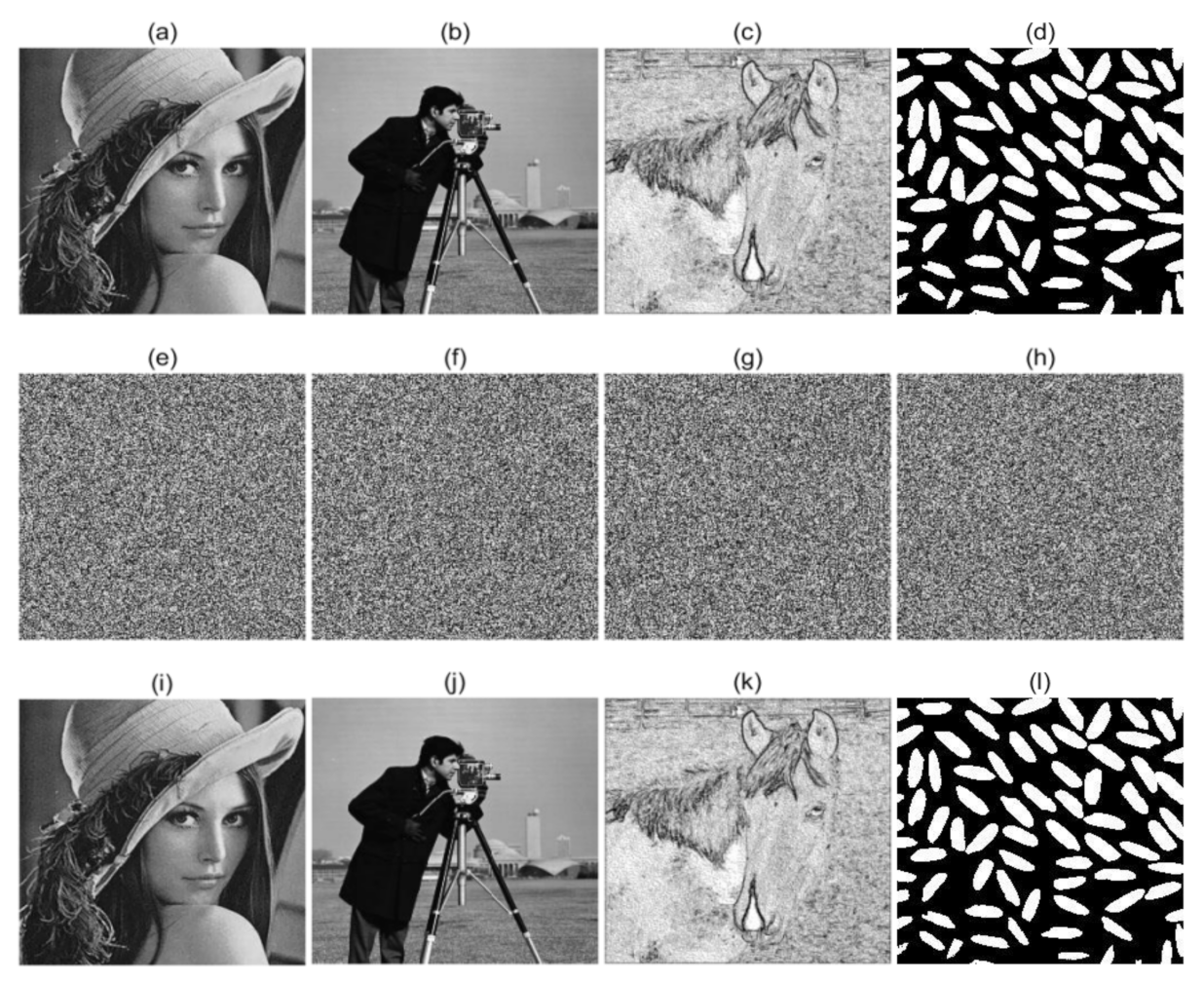
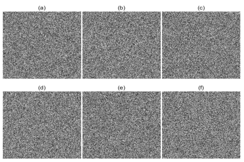
4.1. Encryption and Decryption Tests

The encryption and decryption results of these four images are provided in Figure 10. From Figure 10, we can have that the encrypted images are all unrecognized, which reflects the encrypted image has no features for analysis. For different categories of image, there are almost no differences in the characteristics of the encrypted images. It will be further proved by the following security analysis. Thus, this image encryption algorithm is effective and can be used for all different images. Furthermore, we can find that the plain-images can be decrypt accurately by using the correct keys, which implies that this encryption algorithm is applicable.

4.2. Key Space Analysis

Key space is an important index to evaluate the security of an encryption algorithm. The key space of an encryption algorithm should be at least larger than 2¹²⁸ to resist brute-force attacks [21]. In this LBCCM-IEA, the initial values (x1, x2) and control parameters (a1, a2, p1, p2) can be saw as secret keys. The computing precision is always assumed to be 10⁻¹⁴ in many other studies [3,10,14]; therefore, we set the computing precision be 10⁻¹⁴, as well, in this paper to compare with the key space of these studies at the same scale. The key space of the LBCCM-IEA can be approximately estimated as 10¹⁴ × 10¹⁴ × 10¹⁴ × 10¹⁴ × 10¹⁴ × 10¹⁴ = 10⁸⁴ ≈ 2²⁷⁹, which is much larger than 2¹²⁸, and also larger than the key spaces of refs. [10,12,14,24] under the same precision, which are 2¹⁰⁶, 2²⁷⁷, 2¹⁹⁹, and 2¹⁸⁶, respectively. This result shows that this LBCCM-IEA can effectively resist the brute-force attack.

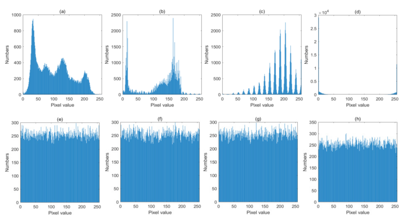
4.3. Histogram Analysis

The distribution of the pixels of a plain-image is always uneven, which leads to the leakage of pixel information. Therefore, the distribution of the encrypted image is a major concern in image encryption. For an ideal encryption algorithm, the histogram of the encrypted image should be uniformly distributed. The histograms of these four groups of plain and encrypted images are shown in Figure 11. From Figure 11, we can easily find that these four ciphered images all have quite flat distributions, which can resist the statistical attack and cipher-only attack effectively.

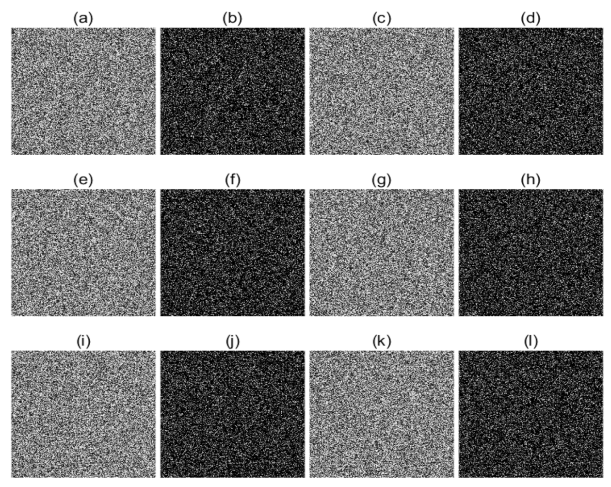
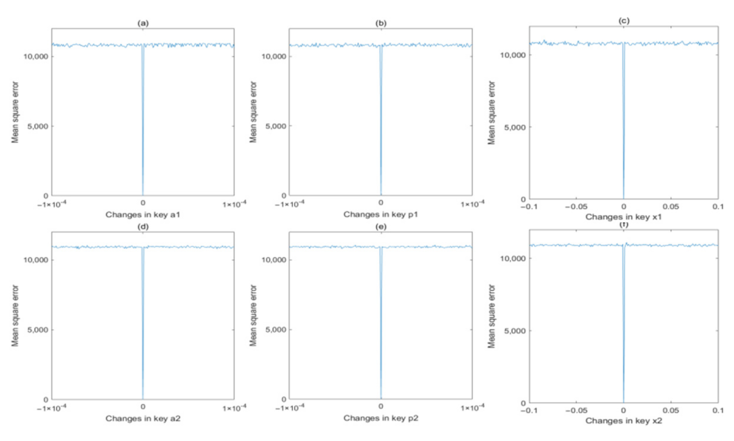
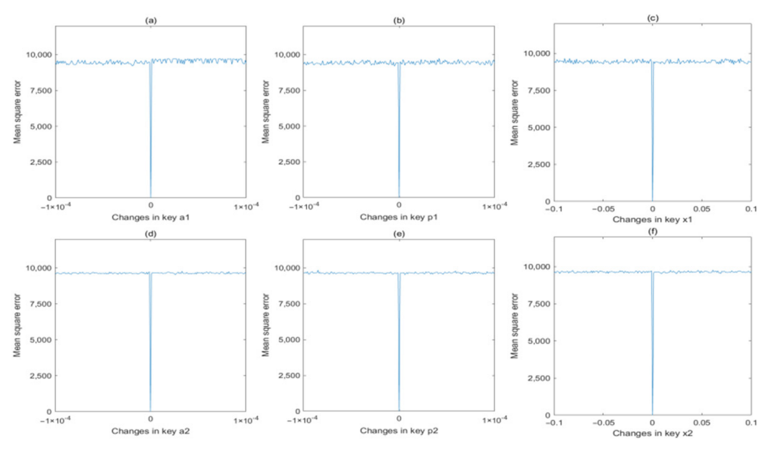
4.4. Key Sensitivity Analysis

An ideal encryption algorithm should be extremely sensitive to its secret keys. In the encryption/decryption process, the encrypted/decrypted images should also be completely different if one of the secret keys has a small change when encrypting/decrypting the same encrypted image. In this experiment, the secret keys are changed by only 10⁻¹⁴ to test the sensitivity. The encryption sensitivity and decryption sensitivity results are shown in Figure 12 and Figure 13, respectively. From Figure 12, we can find that the encryption results are all totally different from the encrypted image in Figure 10e by changing the secret keys with 10⁻¹⁴. These results show that the six security keys are all extremely sensitive in the encryption process. Moreover, Figure 13 shows that the decryption results are all unrecognizable when the secret keys are changing slightly with 10⁻¹⁴, which implies that the cipher image cannot be decrypted effectively. These results show that the six security keys all have ideal sensitivity in the decryption process.

In order to depict the key sensitivity precisely, the following mean square error (MSE) is used to evaluate the sensitivity.

$$MSE=\frac{1}{M}{\sum }_{i=1}^M{\left(y_i-x_i\right)}^2,$$

(30)

where x_i denotes the pixel values of original image, and y_i denotes the pixel values of the changed image. The MSE values are calculated and plotted in Figure 14 and Figure 15 for encryption process and decryption process, respectively. From these two figures, we can find that the MSE value will rapidly change from 0 to a quite large value if the secret key is changing slightly, which proves that these six secret keys are extremely sensitive to both encryption and decryption processes.

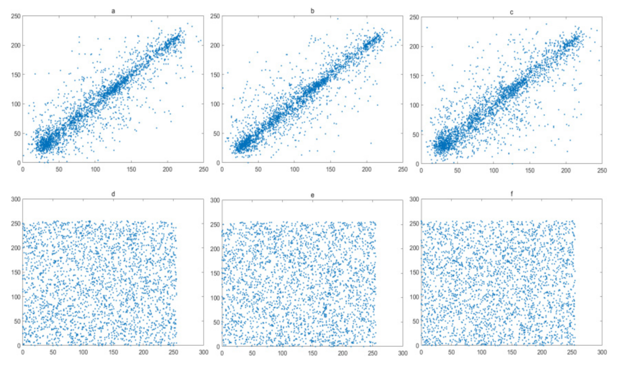
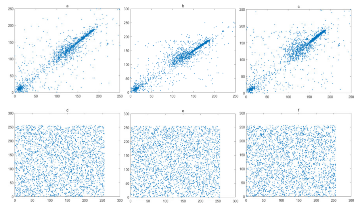
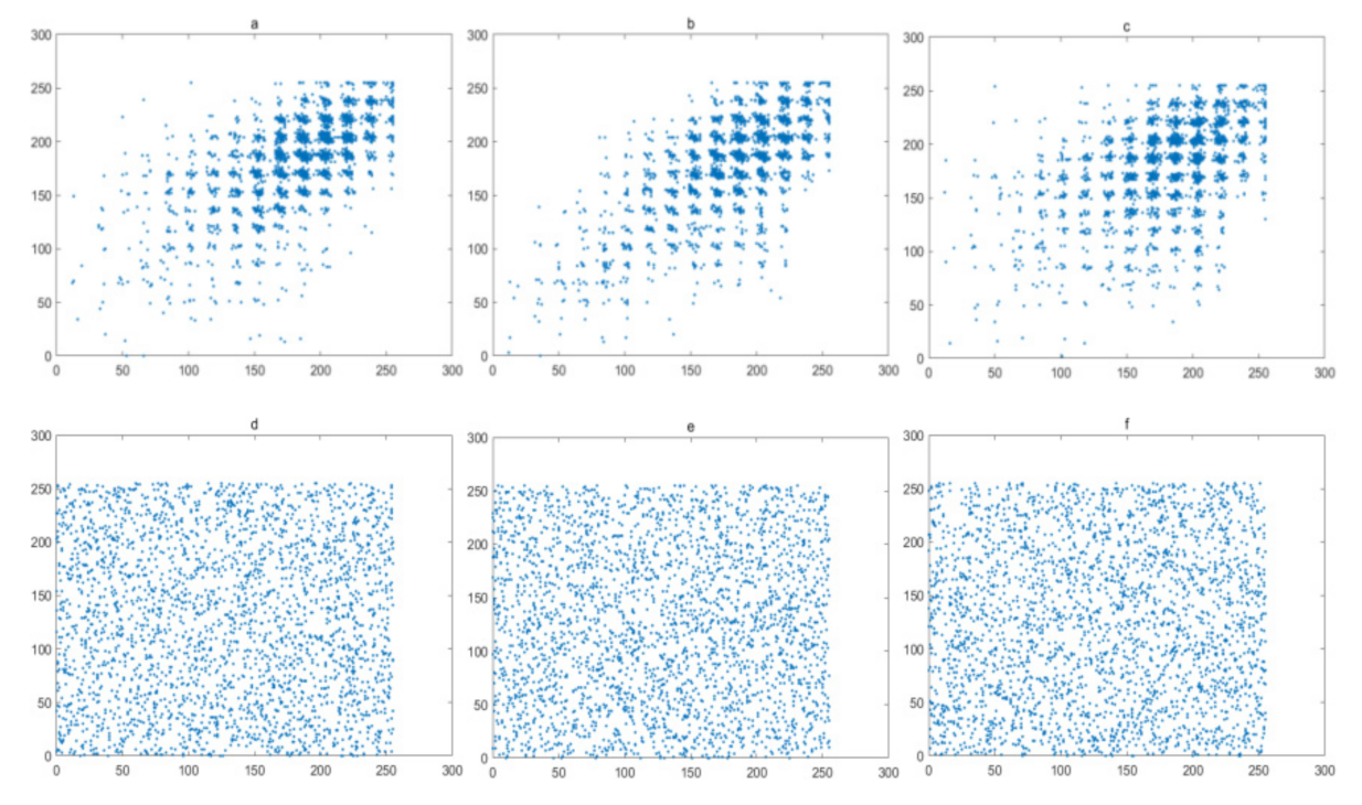
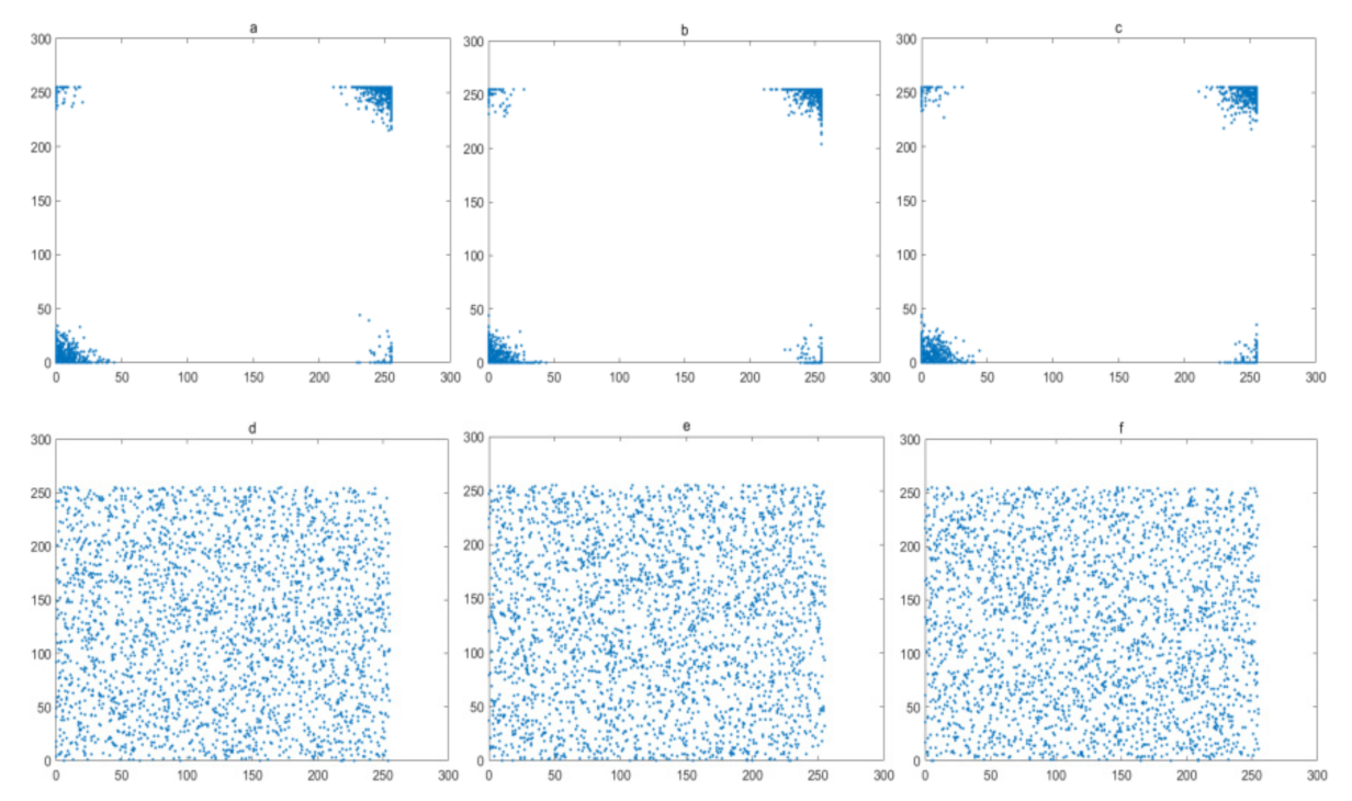
4.5. Correlation Analysis

The pixels of a plain image always has a high correlations with their neighboring pixels. Therefore, reduction of this correlation of adjacent pixels is a basic requirement for a secure image encryption algorithm. In this experiment, 1024 pairs of adjacent pixels along with the horizontal, vertical, and diagonal directions are selected and plotted in Figure 16, Figure 17, Figure 18 and Figure 19, for the Lena image, Cameraman image, Horse image, and Granules image, respectively. As these figures show, the pairs of adjacent pixels of plain-text images are all located on or nearby the diagonal line, which indicates a high correlation between adjacent pixels. However, after encryption, the pairs of adjacent pixels of ciphered images are distributed randomly in the whole domain, which proves that this encryption algorithm is complex enough.

Furthermore, a correlation coefficient is used to measure the correlation between adjacent pixels quantitatively, whose mathematically formula can be written as

$$Corr=\frac{N{\sum }_{i=1}^N\left(x_i\times y_i\right)-{\sum }_{i=1}^N{x}_i\times {\sum }_{i=1}^N{y}_i}{\sqrt{\left(N{\sum }_{i=1}^N{x}_i^2-{\left({\sum }_{i=1}^N{x}_i\right)}^2\right)\times \left(N{\sum }_{i=1}^N{y}_i^2-{\left({\sum }_{i=1}^N{y}_i\right)}^2\right)}},$$

(31)

where x_i and y_i are two sequences with length N. Two sequences are regarded to have a high correlation since the Corr value is close to 1. However, the Corr value close to 0 means two sequences have little correlation with each other. In other words, they are independent of each other.

Table 2. Correlation coefficients analysis.

	Horizontal	Vertical	Diagonal
Original Lena	0.9237	0.9420	0.8906
Encrypted Lena	−0.0034	−0.0079	0.0010
Original Cameraman	0.9333	0.9569	0.9520
Encrypted Cameraman	−0.0094	0.0028	0.0041
Original Horse	0.6425	0.6682	0.5179
Encrypted Horse	−0.0003	0.0249	0.0042
Original Granules	0.8850	0.8743	0.8558
Encrypted Granules	0.0012	−0.0002	0.0013
Ref. [3] Lena	−0.0986	−0.063	0.0509
Ref. [10] Lena	−0.0026	−0.0054	0.0082
Ref. [15] Lena	−0.0119	−0.0087	−0.0045
Ref. [24] Lena	0.0010	0.0042	0.0063

shows the Corr value of adjacent pixel sequences for different directions. From the results, we have that the Corr value of adjacent pixels of plain-text image is quite close to 1, while, after encryption, the Corr value of adjacent pixels of ciphered image is extremely close to 0, which proves that the LBCCM-IEA can greatly break the correlation between adjacent pixels of plain-text image. Compared with other chaos-based schemes, our results are better than the correlation in refs. [3], and they are similar in performances with refs. [10,15,24], which demonstrates that the LBCCM-IEA can effectively resist the correlation attack.

4.6. Information Entropy Analysis

Information entropy is a significant measure to estimate the uncertainty and randomness, which can be used as an important feature in image encryption. The formula of information entropy can be written as

$$H\left(m\right) = -{\sum }_{i=1}^{M}p\left(m_i\right)lo{g}_2 p\left(m_i\right),$$

(32)

where p(m_i) denotes the probability of symbol m_i. For a ciphered image, its entropy value should be very close to the ideal value 8 to ensure its good randomness. The information entropy analysis of plain-text images and the ciphered images in other chaos-based schemes are listed in

Table 3. Information entropy analysis.

	Original Image	Encrypted Image
Lena	7.5984	7.9977
Cameraman	7.0084	7.9971
Horse	6.5645	7.9974
Granules	5.5145	7.9974
Ref. [10] Lena	7.5984	7.9979
Ref. [14] Lena	7.5984	7.9971
Ref. [15] Lena	7.5984	7.9897
Ref. [21] Lena	7.5984	7.9974
Ref. [24] Lena	7.5984	7.9979

. From Table 3, we can find that, for four plain-text images, the entropy values are all quite close to the ideal value 8 after encrypting by the LBCCM-IEA, which means that these ciphered images can be regarded as ideal random images. Compared with other schemes, the entropy value of the ciphered image by this LBCCM-IEA is larger than the entropy values in refs. [14,15], and it is close to the entropy values in refs. [10,21,24], which proves that our algorithm is competitive with other schemes in this sense.

4.7. Resistance to Different Attack Analysis

Differential attack is a popular and effective image analysis method. A secure image encryption algorithm should have a high sensitivity on the plain-text image. To measure the ability to resist differential attack of an encryption algorithm, two statistical indicators are used, named number of pixels change rate (NPCR) and unified average changing intensity (UACI), which can be shown as follows [5].

$$\mathrm{NPCR}=\frac{{\sum }_{i,j}D\left(i,j\right)}{L}\times 100\%,$$

(33)

$$\mathrm{UCAI}=\frac{1}{L}\left[{\sum }_{i,j}\frac{\left|C_1\left(i,j\right)-C_2\left(i,j\right)\right|}{\mathrm{H}}\right]\times 100\%,$$

(34)

where

$$D\left(i,j\right) = \left\{\begin{array}{c}0, C_1\left(i,j\right) = C_2\left(i,j\right)\\ 1, C_1\left(i,j\right) \ne C_2\left(i,j\right)\end{array}\right..$$

(35)

In these formulas, C₁ and C₂ are two different images with the same size. L denotes the number of pixels, and H is the largest allowed pixel value in the images. Setting C₁ and C₂ be the gray images with size 256 × 256, then, we have L = 65,536 and H = 255. The ideal value of NPCR and UACI should be 0.9961 and 0.3346, respectively, for a secure encryption algorithm.

In this text, to measure the sensitivity of the plain-text image, we encrypt two images with only 1-bit difference by using the same keys. Four images are selected as the plain-text image. The NPCR and UACI values are calculated and listed in

Table 4. NPCR and UACI analysis.

	NPCR	UACI
Lena	0.9958	0.3348
Cameraman	0.9964	0.3353
Horse	0.9958	0.3353
Granules	0.9958	0.3330
Ref. [10] Lena	0.9961	0.3220
Ref. [14] Lena	0.9960	0.3343
Ref. [15] Lena	0.9960	0.3349
Ref. [21] Lena	0.9962	0.3347
Ref. [24] Lena	0.9960	0.3340
Ref. [33] Lena	0.9955	0.3327

. Table 4 shows that the NPCR and UACI values are all close to the ideal value for all images, which indicates that the LBCCM-IEA has a high sensitivity to plain-text image, as well as is competitive with other image encryption algorithms in resisting differential attack or chosen-plaintext attack.

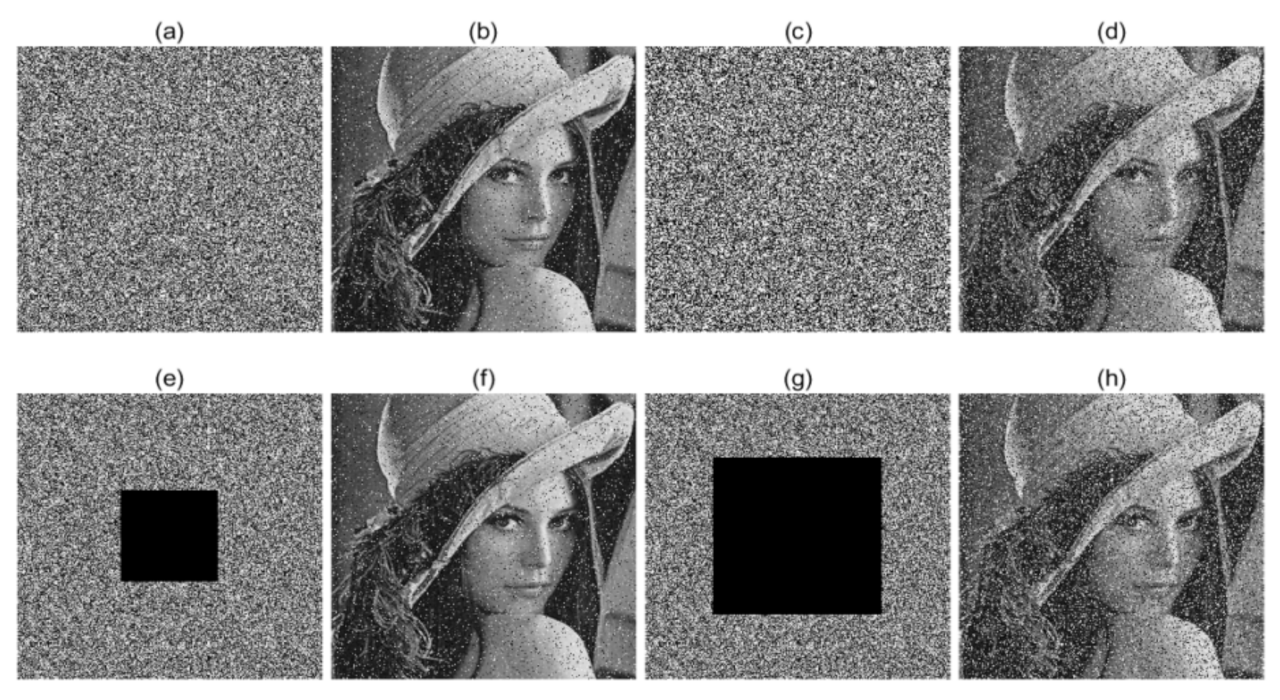
4.8. Robustness Analysis

Data change and loss are inevitable when the images are transmitting in the network, especially in a noisy network. In this experiment, different levels of salt & pepper noise and data loss are considered, and the test results are shown in Figure 20. From Figure 20, we can see that, although the encrypted images are affected by noise or data loss, the decrypted images can still be identified clearly. Based on these results, we can demonstrate that this encryption scheme is robust to noise and data loss, which is suitable for practical uses.

4.9. Computational Complexity Analysis

Computational complexity is also an important measure to evaluate the practicability of an encryption algorithm. The encryption and decryption processes of an image encryption algorithm should be complete in an ideal time. In these tests, the encryption and decryption algorithms are processed by MATLAB 2019 on computer with 3.70 GHz CPU and 7.58 GB memory. The speed of encryption and decryption processes are summarized in

Table 5. Encryption and decryption speed test.

Image Size (256 × 256)	Unit (s)	Speed (Mb/s)
Lena	0.1055	4.7393
Cameraman	0.1053	4.7483
Horse	0.1171	4.2699
Granules	0.0979	5.1073
Ref. [3] Lena	0.1400	3.5714
Ref. [12] Lena	0.9250	0.5405
Ref. [33] Lena	0.1309	3.8197
DES (Lena)	0.6305	0.7930
AES (Lena)	0.2173	2.3010

. From Table 5, we can find that this LBCCM-IEA is faster than other chaotic image encryption algorithms in refs. [2,10,30] in encrypting the same size image, as well as is also much faster than the traditional encryption algorithms DES and AES. Therefore, the proposed LBCCM-IEA is convenient and efficient for practical uses.

5. Conclusions

Chaotic systems have been widely used in image encryption for its complex dynamics. In this paper, we provide a logistic-Baker compound chaotic map. Several experiments are given to prove that the proposed compound chaotic map has ideal characteristics. Furthermore, based on the LB compound chaotic map, a novel image encryption algorithm is proposed. In this algorithm, the compound chaotic function is influenced by the plain-text image, which becomes different when encrypting different images. Thus, this algorithm can resist the differential attack effectively. The proposed encryption algorithm includes three main ideas, shuffling, blocking and substitution. All these steps are related to the sequences generated by the LB compound chaotic map. To prove the security and practicability of this encryption algorithm, several numerical experiments have been taken. All the test results show that the proposed image encryption algorithm has a high security level, and it is quite competitive with other chaos-based image encryption algorithms. The image encryption algorithm proposed in this paper is also valid for color images by dividing the color images into R, G, B three channels.

Recently, quantum computers and their corresponding algorithms have great prospects, and it will indeed become a threat to many encryption algorithms. However, till now, there is no literature that proves that the chaos-based ciphers can be cracked by quantum computing. Thus, in our future work, we will try to further improve the security level of the chaos-based image encryption algorithm, especially to improve the ability of the encryption algorithm to resist quantum attacks.

References

1. Mollaeefar, M.; Sharif, A.; Nazari, M. A novel encryption scheme for colored image based on high level chaotic maps. Multimed. Tools Appl. 2017, 76, 607–629. [Google Scholar] [CrossRef]
2. Pareek, N.K.; Patidar, V.; Sud, K.K. Image encryption using chaotic logistic map. Image Vis. Comput. 2006, 24, 926–934. [Google Scholar] [CrossRef]
3. Ye, G.D.; Wong, W.K. An image encryption scheme based on time-delay and hyperchaotic system. Nonlinear Dyn. 2013, 71, 259–267. [Google Scholar] [CrossRef]
4. Li, C.; Feng, B.; Li, S.; Kurths, J.; Chen, G. Dynamic Analysis of Digital Chaotic Maps via State-Mapping Networks. IEEE Trans. Csyst. I Regul. Pap. 2019, 66, 2322–2335. [Google Scholar] [CrossRef] [Green Version]
5. Chen, C.; Wang, T.; Kou, Y.; Chen, X.; Li, X. Improvement of trace-driven I-Cache timing attack on the RSA algorithm. J. Syst. Softw. 2013, 86, 100–107. [Google Scholar] [CrossRef]
6. Chen, G.; Mao, Y.; Chui, C.K. A symmetric image encryption scheme based on 3D chaotic cat maps. Chaos Solitons Fractals 2004, 21, 749–761. [Google Scholar] [CrossRef]
7. Coppersmith, D. The data encryption standard (DES) and its strength against attacks. IBM J. Res. Dev. 1994, 38, 243–250. [Google Scholar] [CrossRef]
8. Wang, X.; Teng, L.; Qin, X. A novel color image encryption algorithm based on chaos. Signal Process. 2012, 93, 1101–1108. [Google Scholar] [CrossRef]
9. Wang, X.; Wang, S.; Wei, N.; Zhang, Y. A novel chaotic image encryption scheme based on hash function and cyclic shift. IETE Tech. Rev. 2019, 36, 39–48. [Google Scholar] [CrossRef]
10. Liu, L.F.; Miao, S.X. A new simple one-dimensional chaotic map and its application for image encryption. Multimed. Tools Appl. 2017, 77, 21445–21462. [Google Scholar] [CrossRef]
11. Huang, X.L. Image encryption algorithm using chaotic Chebyshev generator. Nonlinear Dyn. 2012, 67, 2411–2417. [Google Scholar] [CrossRef]
12. Li, C.; Luo, G.; Qin, K.; Li, C. An image encryption scheme based on chaotic tent map. Nonlinear Dyn. 2017, 87, 127–133. [Google Scholar] [CrossRef]
13. Short, K.M. Steps toward unmasking secure communications. Int. J. Bifurc. Chaos 1994, 4, 959–977. [Google Scholar] [CrossRef]
14. Ye, G.; Pan, C.; Huang, X.; Mei, Q. An efficient pixel-level chaotic image encryption algorithm. Nonlinear Dyn. 2018, 94, 745–756. [Google Scholar] [CrossRef]
15. Liu, Q.; Liu, L.F. Color image encryption algorithm based on DNA coding and double chaos system. IEEE Access 2020, 8, 83596. [Google Scholar] [CrossRef]
16. Wang, X.Y.; Lin, S.J.; Li, Y. A chaotic image encryption scheme based on cat map and MMT permutation. Mod. Phys. Lett. B 2019, 33, 1950326. [Google Scholar] [CrossRef]
17. Liu, Y.; Zhang, J.D. A multidimensional chaotic image encryption algorithm based on DNA coding. Multimed. Tools Appl. 2020, 79, 21579–21601. [Google Scholar] [CrossRef]
18. Chai, X.; Wu, H.; Gan, Z.; Han, D.; Zhang, Y.; Chen, Y. An efficient approach for encrypting double color images into a visually meaningful cipher image using 2D compressive sensing. Inf. Sci. 2020, 563, 91–110. [Google Scholar] [CrossRef]
19. Chai, X.; Bi, J.; Gan, Z.; Liu, X.; Zhang, Y.; Chen, Y. Color image compression and encryption scheme based on compressive sensing and double random encryption strategy. Signal Process. 2020, 176, 107684. [Google Scholar] [CrossRef]
20. Alghafis, A.; Firdousi, F.; Khan, M.; Batool, S.I.; Amin, M. An efficient image encryption scheme based on chaotic and Deoxyribonucleic acid sequencing. Math. Comput. Simul. 2020, 177, 441–466. [Google Scholar] [CrossRef]
21. Luo, Y.; Yu, J.; Lai, W.; Liu, L. A novel chaotic image encryption algorithm based on improved baker map and logistic map. Multimed. Tools Appl. 2019, 78, 22023–22043. [Google Scholar] [CrossRef]
22. Ye, G.D. Image scrambling encryption algorithm of pixel bit based on chaotic map. Pattern Recognit. Lett. 2010, 31, 347–354. [Google Scholar] [CrossRef]
23. Oravec, J.; Turán, J.; Ovseník, Ľ.; Huszaník, T. A chaotic image encryption algorithm robust against phase space reconstruction attacks. Acta Polytech. Hung. 2019, 16, 37–57. [Google Scholar]
24. Li, R.Z.; Liu, Q.; Liu, L.F. Novel image encryption algorithm based on improved logistic map. IET Image Process. 2019, 13, 125–134. [Google Scholar] [CrossRef]
25. Hua, Z.Y.; Zhang, Y.X.; Zhou, C.Y. Two-dimensional Modular Chaotification System for improving chaotic complexity. IEEE Trans. Signal Process. 2020, 68, 1937–1949. [Google Scholar] [CrossRef]
26. Mansouri, A.; Wang, X.Y. A novel one-dimensional chaotic map generator and its application in a new index representation-based image encryption scheme. Inf. Sci. 2021, 563, 91–110. [Google Scholar] [CrossRef]
27. Liu, L.F.; Miao, S.X. Delay-introducing method to improve the dynamical degradation of a digital chaotic map. Inf. Sci. 2017, 396, 1–13. [Google Scholar] [CrossRef]
28. Zhang, S.J.; Liu, L.F. A novel image encryption algorithm based on SPWLCM and DNA coding. Math. Comput. Simul. 2021, 190, 723–744. [Google Scholar] [CrossRef]
29. Li, X.; Zhang, G.J.; Zhang, X.Y. Image encryption algorithm with compound chaotic maps. J. Ambient. Intell. Humaniz. Comput. 2015, 6, 563–570. [Google Scholar] [CrossRef]
30. Wang, X.Y.; Zhang, J.J.; Cao, G.H. An image encryption algorithm based on ZigZag transform and LL compound chaotic system. Opt. Laser Technol. 2019, 119, 105581. [Google Scholar]
31. Lu, Q.; Zhu, C.X.; Wang, G.J. A novel S-Box design algorithm based on a new compound chaotic system. Entropy 2019, 21, 1004. [Google Scholar] [CrossRef] [Green Version]
32. Hua, Z.; Zhu, Z.; Yi, S.; Zhang, Z.; Huang, H. Cross-plain colour image encryption using a two-dimensional logistic tent modular map. Inf. Sci. 2020, 546, 1063–1083. [Google Scholar] [CrossRef]
33. Askar, S.S.; Karawia, A.A.; Al-Khedhairi, A.; Al-Ammar, F.S. An algorithm of image encryption using logistic and two-dimensional chaotic economic maps. Entropy 2019, 21, 44. [Google Scholar] [CrossRef] [Green Version]
34. Pan, H.L.; Lei, Y.M.; Jian, C. Research on digital image encryption algorithm based on double logistic chaotic map. Eurasip J. Image Video Process. 2018, 142. [Google Scholar] [CrossRef]
35. Pincus, S.M. Approximate entropy as a measure of system complexity. Proc. Nat. Acad. Sci. USA 1991, 88, 2297–2301. [Google Scholar] [CrossRef] [Green Version]
36. Bandt, C.; Pompe, B. Permutation Entropy: A Natural Complexity Measure for Time Series. Phys. Rev. Lett. 2002, 88, 174102. [Google Scholar] [CrossRef]
37. Alireza, J.; Abdolrasoul, M. Image encryption using chaos and block copher. Comput. Inform. Sci. 2011, 4, 172–185. [Google Scholar]
38. Won, Y.J.; Hyoungshick, K. An image encryption scheme with a pseudorandom permutation based on chaotic maps. Commun. Non. Sci. Num. Simulat. 2010, 15, 3998–4006. [Google Scholar]
39. Zhang, M.; Tong, X.J. A new chaotic map based image encryption schemes for several image formats. J. Syst. Softw. 2014, 98, 140–154. [Google Scholar] [CrossRef]
40. Wolf, A.; Swift, J.B.; Swinney, H.L.; Vastano, J.A. Determining lyapunov exponents from a time series. Physica 1985, 16, 285–317. [Google Scholar] [CrossRef] [Green Version]
41. Rukhin, A.; Soto, J.; Nechvatal, J.; Smid, M.; Barker, E. A Statistical Test Suite for Random and Pseudorandom Number generators for Cryptographic Applications. NIST Spec. Publ. 800-22 2001. [Google Scholar] [CrossRef]
Figure 1. (a) ApEn analysis of the logistic sequence; (b) PE analysis of the logistic sequence.
Mathematics 09 02778 g001
Figure 2. Complexity analysis of Baker sequence; (a) ApEn; (b) PE.
Mathematics 09 02778 g002
Figure 3. Trajectories of the LB compound chaotic map: (a) x-dimensional variable (b) y-dimensional variable (sub-figures are the partial enlargement).
Mathematics 09 02778 g003
Figure 4. Bifurcation diagram of the LB compound chaotic map: (a) x-dimensional variable; (b) y-dimensional variable.
Mathematics 09 02778 g004
Figure 5. Auto-correlation function of the LB compound chaotic map.
Mathematics 09 02778 g005
Figure 6. ApEn analysis of the LB compound chaotic map: (a) ApEn comaprison with logistic map (b) ApEn comparison with Baker map.
Mathematics 09 02778 g006
Figure 7. PE analysis of the LB compound chaotic map: (a) PE comaprison with logistic map (b) PE comparison with Baker map.
Mathematics 09 02778 g007
Figure 8. Lyapunov exponent analysis of the LB compound chaotic map: (a,b) x-dimensional variable; (c,d) y-dimensional variable.
Mathematics 09 02778 g008
Figure 9. The flowchart of the LBCCM-IEA.
Mathematics 09 02778 g009
Figure 10. Encryption and decryption test (ad). Original images; (eh) encrypted images; (il) decrypted images.
Mathematics 09 02778 g010
Figure 11. Histograms of images (ad). Original images: Lena, Cameraman, Horse and Granules; (eh) encrypted images: Lena, Cameraman, Horse and Granules.
Mathematics 09 02778 g011
Figure 12. Key sensitivity analysis. Encrypted image with: (a) a1 = 4 − 10−14; (c) a2 = 3.77 − 10−14; (e) p1 = 0.499 − 10−14; (g) p2 = 0.37 − 10−14; (i) x1 = 0.1260 − 10−14; (k) x2 = 0.3265 − 10−14. (b) Difference between (a) and Figure 10e; (d) difference between (c) and Figure 10e; (f) difference between (e) and Figure 10e; (h) difference between (g) and Figure 10e; (j) difference between (i) and Figure 10e; (l) difference between (k) and Figure 10e.
Mathematics 09 02778 g012
Figure 13. Key sensitivity analysis. Decrypted image with (a) a1 = 4 − 10−14; (b) a2 = 3.77 − 10−14; (c) p1 = 0.499 − 10−14; (d) p2 = 0.37 − 10−14; (e) x1 = 0.1260 − 10−14; (f) x2 = 0.3265 − 10−14.
Mathematics 09 02778 g013
Figure 14. MSE analysis in encryption process for different keys: (a) a1; (b) p1; (c) x1; (d) a2; (e) p2; (f) x2.
Mathematics 09 02778 g014
Figure 15. MSE analysis in decryption process for different keys: (a) a1; (b) p1; (c) x1; (d) a2; (e) p2; (f) x2.
Mathematics 09 02778 g015
Figure 16. Correlation analysis of Lena image: (ac) horizontal, vertical and diagonal direction of plain-text image; (df) horizontal, vertical and diagonal direction of cipher.
Mathematics 09 02778 g016
Figure 17. Correlation analysis of Cameraman image: (ac) horizontal, vertical and diagonal direction of plain-text image; (df) horizontal, vertical and diagonal direction of cipher.
Mathematics 09 02778 g017
Figure 18. Correlation analysis of Horse image: (ac) horizontal, vertical and diagonal direction of plain-text image; (df) horizontal, vertical and diagonal direction of cipher.
Mathematics 09 02778 g018
Figure 19. Correlation analysis of Granules image: (ac) horizontal, vertical and diagonal direction of plain-text image; (df) horizontal, vertical and diagonal direction of cipher.
Mathematics 09 02778 g019
Figure 20. Robustness analysis (a) 10.00% salt & pepper noise of ciphered Lena; (b) decrypted result of (a); (c) 30.00% salt & pepper noise of ciphered Lena; (d) decrypted result of (c); (e) 10.00% data loss of ciphered Lena; (f) decrypted result of (e); (g) 30.00% data loss of ciphered Lena; (h) decrypted result of (g).
Mathematics 09 02778 g020