Controlling Chaos in Van Der Pol Dynamics Using Signal-Encoded Deep Learning

Abstract

Controlling nonlinear dynamics is a long-standing problem in engineering. Harnessing known physical information to accelerate or constrain stochastic learning pursues a new paradigm of scientific machine learning. By linearizing nonlinear systems, traditional control methods cannot learn nonlinear features from chaotic data for use in control. Here, we introduce Physics-Informed Deep Operator Control (PIDOC), and by encoding the control signal and initial position into the losses of a physics-informed neural network (PINN), the nonlinear system is forced to exhibit the desired trajectory given the control signal. PIDOC receives signals as physics commands and learns from the chaotic data output from the nonlinear van der Pol system, where the output of the PINN is the control. Applied to a benchmark problem, PIDOC successfully implements control with a higher stochasticity for higher-order terms. PIDOC has also been proven to be capable of converging to different desired trajectories based on case studies. Initial positions slightly affect the control accuracy at the beginning stage yet do not change the overall control quality. For highly nonlinear systems, PIDOC is not able to execute control with a high accuracy compared with the benchmark problem. The depth and width of the neural network structure do not greatly change the convergence of PIDOC based on case studies of van der Pol systems with low and high nonlinearities. Surprisingly, enlarging the control signal does not help to improve the control quality. The proposed framework can potentially be applied to many nonlinear systems for nonlinear controls.

1. Introduction

Controlling chaos and nonlinear dynamics is a long-standing issue in various engineering disciplines, including aerospace systems design [1]; chemical operations [2]; robotics [3]; biological sciences [4]; mechatronics [5]; and, in particular, microelectronics [6], especially for circuits systems involving semiconductors that elicit nonlinearity for signal controls [7,8]. In mathematics, chaos is characterized by underlying patterns and deterministic laws that are highly sensitive to the initial conditions in dynamical systems and sometimes manifest as solutions for a differential equation (or a representation of the system) that do not converge to a stationary or periodic function of time but continue to exhibit seemingly unpredictable behavior [9]. Controlling chaotic nonlinear dynamics has a simple objective: implementing the desired command in the system to make it behave “as we wish” or at least make it predictable so that helpless impotence can be eliminated. However arduous [10], nonlinear control problems are ubiquitous in nature, occurring in fluid flows, heartbeat irregularities, weather, and climate [11,12,13]. Hence, addressing such a problem is worthwhile.

Traditionally, proportional–integral–derivative controllers (PID) are used for controlling nonlinear systems [14,15], where closed-loop feedback errors are tuned using linearized versions of nonlinear, chaotic equations seeking to come as close to the targeted trajectory as possible [16]. Such methods remain commonplace in industry. Notably, with such wide applications, PID control experiences sluggish and systematic performance due to the integral term, and increasing the order can lead to system instability [17]. Admittedly, reducing PID to PI (proportional–integral) or P (proportional) might either increase the speed or system stability, but neither can learn the features of nonlinear systematic data, which allows more advanced self-adjust control behavior. Another common approach is to model the chaotic behaviors as periodic ones and implement trigonometric commands in hopes of producing predictable periodic system behavior [18]. Model predictive controllers incorporate statistics seeking good results for fuzzy systems [19].

In recent decades, the skyrocketing usage of big data, assisted by advanced computing technologies such as GPU computing [20], has led to the enhancement of machine learning algorithms—specifically, deep neural networks [21]. Deep neural networks can learn and capture features from highly nonlinear data for accurate predictions, indicating their huge potential and attracting a great deal of attention in various fields. Encoding physics information in the losses of a deep neural network (NN) promises the faster, accurate learning of physics with neural networks by respecting the basic laws of physics using less labeled data, commonly recognized as Physics-Informed Neural Networks (PINNs) [22,23]. One of the most celebrated characteristics of PINNs is their ability to learn from sparse data [24]. Upon the proposed PINN framework, various PINNs designed for disparate engineering applications have emerged. Perhaps their most renowned use is in predicting fluid fields [25,26], but other notable uses include electronics applications [27,28]. Notably, there have been a few attempts to use the PINN-based method to learn and predict nonlinear dynamical systems and chaos [29,30,31,32], with a notable good attempt by Antonelo et al. [33] to modify PINN to adjust systematic controls based on the predictions of PINN. Furthermore, PINN has been used to learn controls for a series of optimal planar orbit transfer problems [34]. However, most applications focus on the “learning” and “discovery” of dynamics with PINNs, while few actually focus on “controlling” the system—that is, guiding the system to behave as human-desired signals. Attempts have been made to use NN for controls as far back as the 1990s [35,36,37], but these attempts were limited to replacing a block or parts of the closed-loop framework with an NN rather than directly using the NN-based framework for signal controls.

Acknowledging the limitations of PINNs and other NN-based controls, a question emerges: can control signals be incorporated in PINNs for chaotic nonlinear dynamical systems? To investigate this, we focus on a system proposed by Balthasar van der Pol in 1920 when he was an engineer working for the Philips Company (in the Netherlands) while studying oscillating circuits [38,39,40]. The van der Pol system exhibits highly chaotic behavior encompassing wide applications in biology, biochemistry, and microelectronics [41,42,43]. 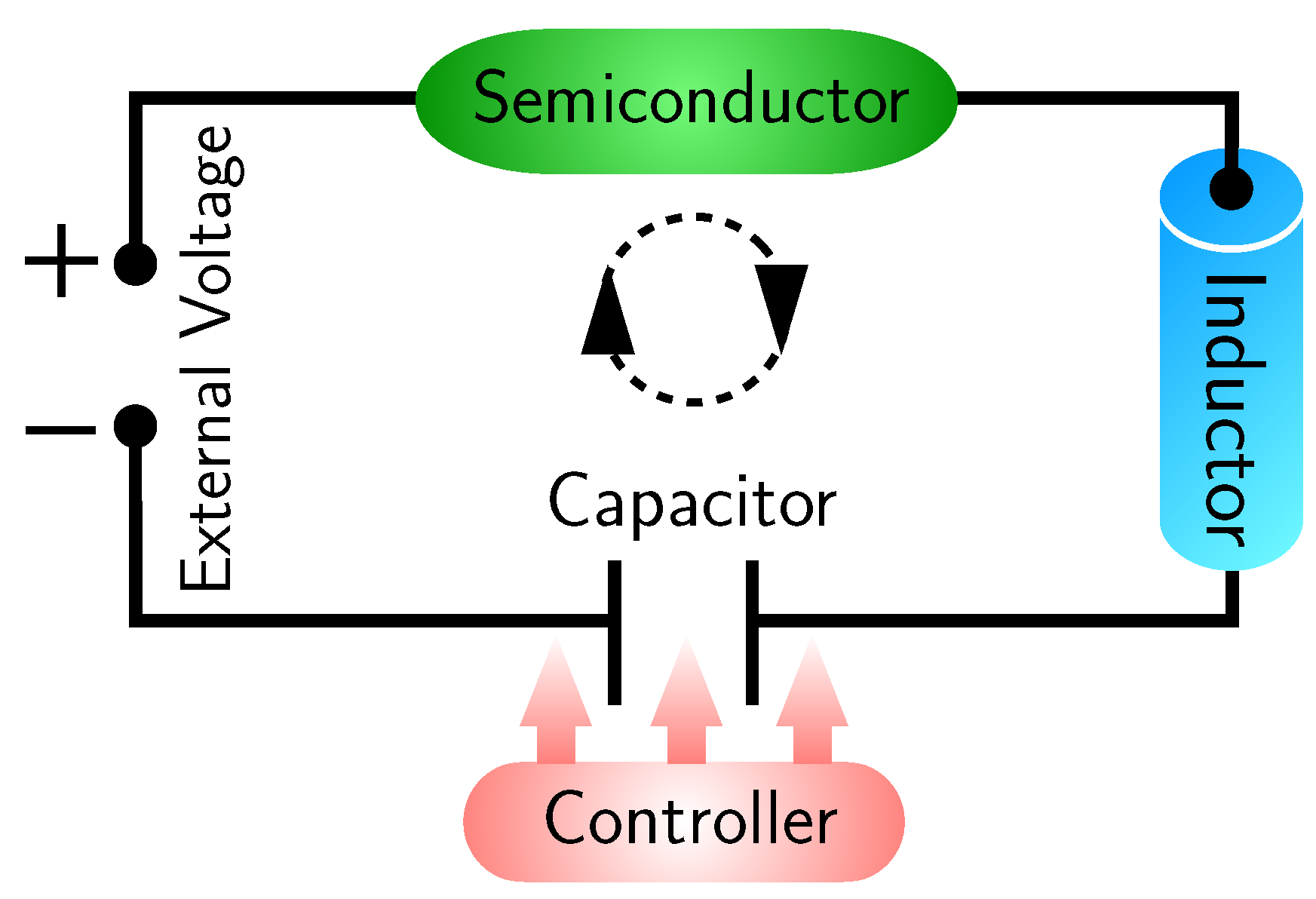The traditional control of the van der Pol system usually includes linearizing the system and adding a forcing term based on the linearized system to impose control [44,45,46,47]. A basic setup of the oscillating van der Pol circuit is illustrated in Figure 1: an external voltage excites the circuit, inducing a current that can be converted to a charge through the capacitor [48]. If the semiconductor as indicated in green is equipped, the circuit will display highly nonlinear behavior that is hard to control and predict. Designing a controller (red block) for controlling the chaotic, nonlinear behavior in such circuits is our main goal.

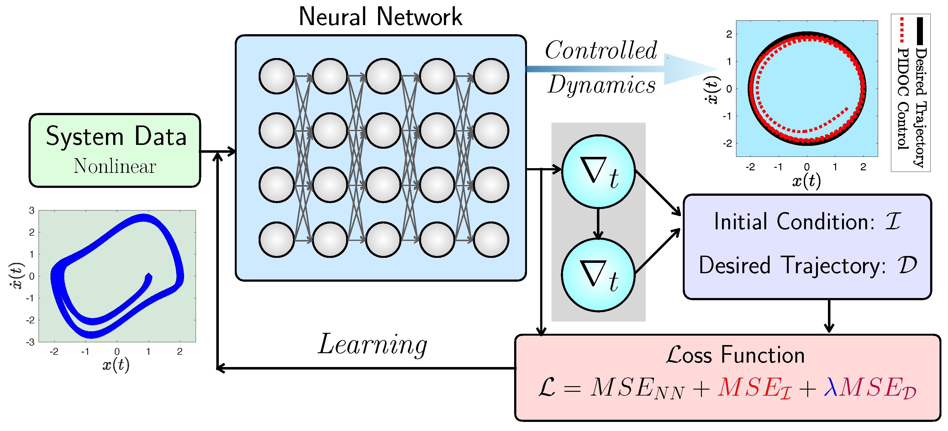
Inspired by [47] and seeking to compare the application of PINNs [22] to the van der Pol system, we propose Physics-Informed Deep Operator Control (PIDOC), a PINN-based control method that incorporates into the loss function of a PINN the generation losses of NN, the desired control signal, and the initial position of the system. The framework is tested based on its behavior and its ability to deal with the highly nonlinear system, while the hyperparameters are also investigated for the better interpretation and potential application of PIDOC.

The manuscript is arranged as follows: in Section 2 we first formulate the problem of a van der Pol system and controls (Section 2.1), elaborating the basic system setup in Section 2.2. In Section 3, the detailed methodologies of formulating and learning with PIDOC are described, consisting of deep learning (Section 3.1) and physics-informed control (Section 3.2). The numerical experiments conducted are briefly summarized in Section 3.3. Next, Section 4 shows the results and discussion of PIDOC. 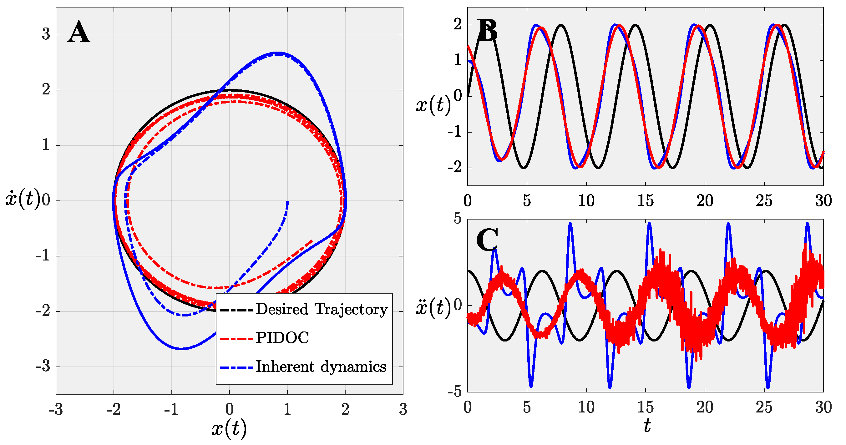Section 4.1 analyzes the behavior of PIDOC given a benchmark problem followed by an in-depth estimation of the nonlinearity of trajectory convergence in Section 4.2, the estimation of the amplitude of control signals (Section 4.2.1), the influence of initial positions (Section 4.2.2), and a nonlinearity analysis (Section 4.2.3). The hyperparameters of the NN (Section 4.3.1) and the weight of the control signal in PINN is described in Section 4.3.2.

2. Problem Formulation

The nonlinear control of the chaotic van der Pol system problem here is mainly inspired by the work of Cooper et al. [47], with a clear problem objective: the successful implementation of a desired trajectory in the van der Pol system.

2.1. Van Der Pol Dynamics

The van der Pol dynamics describe the oscillatory behavior of a class of nonlinear equations [38], originally describing the oscillating circuits with semiconductors introduced in Section 1, as expressed in Equation (1):

$$\frac{d^{2}x}{d{t}^2}-\mu (1-x^2)\frac{dx}{dt}+x=0$$

(1)

where if $x\left(t\right)$ is referred to as state, $\dot{x}\left(t\right)$ is the rate and $\ddot{x}\left(t\right)$ is the acceleration; $\mu$ is a scalar parameter indicating the nonlinearity and the strength of the damping.

The equation exhibits an oscillatory behavior but with a non-constant amplitude, representing an invariant trajectory set called a “limit cycle” [47]. System trajectories converge to these invariant orbits given any initial conditions, as shown in Figure 2: Given six different initial points, all converge to the non-constant limit cycle with a changing velocity relative to their positions, indicating a non-stable phase. The robustness of the nonlinear phase suffers, as the system is “trapped” in the set until the control signals cease, indicating the robustness of the inherent dynamics.

As indicated in Section 1, the main goal is to control such nonlinear behavior. Seeking to produce a fixed-amplitude oscillation, traditional control methods commonly add forcing functions to the nonlinear equation as in Equation (2), which allows linear time-invariant (LTI) feedback control based on a linearized version of the system equation, as in [47]:

$$\frac{d^{2}x}{d{t}^2}-\mu (1-x^2)\frac{dx}{dt}+x=F\left(t\right)$$

(2)

However, in this manuscript such an attempt is not adopted. Our goal is to control the unsteady state of oscillating dynamics by learning from the original van der Pol equation. Such an attempt will not suffer from the errors of linearization as in traditional methods such as PI or PID controllers [14,15,49], and neither does it accumulate errors in the integrator of PID control. Furthermore, the NN-based control PIDOC is able to capture the nonlinear chaotic features directly from the van der Pol system data (through the capacitor in Figure 1). The optimization of minimizing losses is an innate feedback process to the framework for the control as the errors are reduced each iteration, while the feed-forward control signal is found using the predictions from the learning of the NN. For system controls, a classical approach would be to input a sinusoidal or other triangular functions through modifying $F\left(t\right)$ in Equation (2). Meanwhile, we incorporate such a signal as an external supervision [50] added to PIDOC in this research.

2.2. System Simulation

Depicting and emulating the system as described in Figure 1 are both achieved using a simulation of the van der Pol system that generates nonlinear data which are fed into the PIDOC for control. In the classical definition of a neural network, such data are considered as training data used by the neural network to help it “learn” and “predict”. Here, the Python differential equation solver odeint, part of SciPy library, is adopted to simulate the van der Pol equation [51]. The odeint is a library containing advanced numerical methods for solving differential equations, especially for initial value problems [52]. Compared with other solvers such as scipy.integrate.solve_ivp, odeint is able to generate data with a higher smoothness [53], promising a “cleaner” data feed for training and learning. In this research, the van der Pol equation is solved for $t=30$ and interpolated with 3000 points using Equation (1). The error control parameters of the solvers rtol and atol are chosen as ${10}^{-6}$ and ${10}^{-10}$, respectively [51].

3. Methodology and Algorithm

In this section, we will introduce the basic setup of PIDOC, employing PINN as the initial position (denoted by $\mathcal{I}$) and control signal (denoted by $\mathcal{D}$, meaning desired trajectory) encoded within the NN losses for accurate controls.

3.1. Deep Learning

PIDOC controls nonlinear systems based on “learning” from chaotic data for the output of a prediction as the control; this is enabled by a deep neural network (DNN). For the van der Pol system, the DNN is formulated as:

$$\begin{array}{c}\hfill x_{pred}=(K_L\circ {\sigma }_L\circ \dots \circ K_1\circ {\sigma }_1\circ K_0)t\end{array}$$

(3)

where the DNN outputs a desired trajectory $x_{pred}$ given an input of the specific time series t. $K_1,K_2,\dots ,K_L$, are linear layers; ${\sigma }_1,{\sigma }_2,\dots ,{\sigma }_L$ are the activation functions, where PIDOC employs tanh activation functions. For PIDOC, the NN takes time t as the input layer $K_0$ to transmit through $(L-1)$th hidden layers to generate an output $x_{pred}$ through the output layer $K_L$, supervised from the chaotic data of the van der Pol system $x_{train}$. Here, let ${\mathcal{N}}^L\equiv (K_L\circ {\sigma }_L\circ \dots \circ K_1\circ {\sigma }_1\circ K_0)$ denote the Lth-layer NN.

The DNN corresponding to Equation (3) is commonly recognized as a combination of three layers: input, hidden, and output. This is where the neurons are connected and is commonly known as a feed-forward NN, which is defined recursively as

$$\begin{array}{cc}\hfill \mathrm{Input}\mathrm{layer}:K_0\left(t\right)& =t\subset {\mathbb{R}}^{d_{in}}\hfill \\ \hfill \mathrm{Hidden}\mathrm{layer}:K_{\mathfrak{L}}\left(t\right)& =\sigma \left({\mathbf{w}}_{\mathfrak{L}}{K}_{\mathfrak{L}-1}\left(t\right)+{\mathbf{b}}_{\mathfrak{L}}\right)\subset {\mathbb{R}}^{{\mathcal{K}}^{\mathfrak{L}}},\mathrm{for}1\le \mathfrak{L}\le L-1\hfill \\ \hfill \mathrm{Output}\mathrm{layer}:K_L\left(t\right)& ={\mathbf{w}}_L{K}_{L-1}+{\mathbf{b}}_L\subset {\mathbb{R}}^{d_{out}},\left(x_{pred}\equiv K_L\left(t\right)\right)\hfill \end{array}$$

(4)

For the NN ${\mathcal{N}}^L\left(t\right):{\mathbb{R}}^{d_{in}}⟶{\mathbb{R}}^{d_{out}}$, the input time series t is transmitted to the linear input layer $K_0$ forward through hidden layers from a linear model with ${\mathbf{w}}_{\mathfrak{L}}$ as weights and ${\mathbf{b}}_{\mathfrak{L}}$ as biases activated through an activation function tanh. This generates an output through $K_L$ for NN predictions $x_{pred}$ and can also be interpreted as the controlled dynamics. It can be seen that there are ${\mathcal{K}}^{\mathfrak{L}}$ neurons in the $\mathfrak{L}$th layer $\left({\mathcal{K}}^0=d_{in}\&{\mathcal{K}}^L=d_{out}\right)$; the weights and biases are denoted by ${\mathbf{w}}_{\mathfrak{L}}\subset {\mathbb{R}}^{{\mathcal{K}}^{\mathfrak{L}}\times {\mathcal{K}}^{\mathfrak{L}-1}}$ and ${\mathbf{b}}_{\mathfrak{L}}\subset {\mathbb{R}}^{{\mathcal{K}}^{\mathfrak{L}}}$ [54]. Note that the visualization of the NN is shown in the blue box in Figure 3.

In the PIDOC formulation, a supervised machine learning problem is defined, where the NN learning is enabled through the supervision of external training data as a formulation for minimizing the loss function, meaning that the NN can capture data structures through this optimization process, wherein traditional NN approaches $\mathcal{L}$ usually involve the differences (errors) between the NN predictions and training data. Let $\mathcal{L}=\mathcal{L}(t,\mathbf{p})$ denote the loss function, where t is the input time series and $\mathbf{p}$ is the parameter vector containing the formations of $\mathcal{I}$, $\mathcal{D}$, and NN. If no external constraints or bounds are enforced, the optimization problem hence takes the form:

$$\underset{t\subset {\mathbb{R}}^{d_{out}}}{min}\mathcal{L}(t,\mathbf{p})$$

(5)

Minimizing $\mathcal{L}$ requires recursive iterations over the NN, as in Equation (4). The information encoded in $\mathcal{L}$ is reduced during iterations given the optimization methods, where we adopt the limited-memory Broyden–Fletcher–Goldfarb–Shanno optimization algorithm, a quasi-Newton method (L-BFGS-B in TensorFlow 1.x) [55,56]. The optimization is carried over the iteration loop from the blue box (NN) to the purple box ($\mathcal{I}$ & $\mathcal{D}$) to the red box ($\mathcal{L}$), as shown in Figure 1. The maximum iterations are set as $2\times {10}^5$. In the PIDOC formulation, $\mathcal{L}$ is calculated based on the mean square errors of the encoded information, as shown in Section 3.2.

3.2. Physics-Informed Control

The implementation of control signals is enabled through the physics information inserted into the loss function, mimicking the strategy of PINNs, but instead aiming to execute a command on the training data so as to tune the system to a stable stage. The formulation of the loss function includes the mean square errors (MSEs) of the NN generation $MS{E}_{NN}$, the initial conditions $MS{E}_{\mathcal{I}}$, and the desired trajectory $MS{E}_{\mathcal{D}}$ multiplied by a Lagrangian multiplier $\lambda$ so as to enlarge the control signal:

$$\begin{array}{c}\hfill \mathcal{L}=MS{E}_{NN}+MS{E}_{\mathcal{I}}+\lambda MS{E}_{\mathcal{D}}\end{array}$$

(6)

where the NN generation errors $MS{E}_{NN}$ are computed as the MSE for the difference between the training data $x_{train}$ and the NN-predicted output $x_{pred}$:

$$MS{E}_{NN}:=\frac{1}{N}\sum _{i=1}^N{\left|x_{train}-x_{pred}\right|}^2$$

(7)

The initial position loss $MS{E}_{\mathcal{I}}$ is computed as the MSE between the given initial conditions of $\mathcal{D}$ with the system predictions $x_{pred}$ at the initial:

$$MS{E}_{\mathcal{I}}:=\frac{1}{N}\sum _{i=1}^N{\left|x_{pred}^0-x_{\mathcal{D}}^0\right|}^2$$

(8)

where $x_{pred}^0$ denotes the initial position (0th in the array in Python) of NN prediction; $x_{\mathcal{D}}^0$ denotes the initial position of desired trajectory.

The control signal losses $MS{E}_{\mathcal{D}}$ are the mean square error of the differences between the zero- and second-order derivatives of the position between the NN predictions (output) and the desired control trajectories. In short, $MS{E}_{\mathcal{D}}$ imposes our desired control on PIDOC:

$$MS{E}_{\mathcal{D}}:=\frac{1}{N}\sum _{i=1}^N{\left|\left(\frac{d{x}_{\mathcal{D}}^2}{d{t}^2}-\frac{d{x}_{pred}^2}{d{t}^2}\right)+\left(x_{\mathcal{D}}-x_{pred}\right)\right|}^2$$

(9)

Here, $MS{E}_{\mathcal{D}}$ incorporates the control, while the multiplication of $\lambda$ in Equation (6) allows us to tune the weight of the signal. The optimization problem formulated in Equation (5) can hence be considered as a multi-objective gradient-based optimization, as the objective of control can be tuned through $\lambda$. Specifically, it has been reported that the limited-memory BFGS method has been widely applied for large-scale unconstrained optimization [57].

The classical control approach uses a square wave or triangular function as signals [58]. For circuit systems specifically, applying a sinusoidal wave is a common practice, as in the work of Cooper et al. [47]. Here, for applications of PIDOC, we also applied a sinusoidal wave multiplied by an adjustable multiplier $\mathsf{\Lambda }$ to control the amplitude of the phase:

$$x_{\mathcal{D}}\left(t\right)=\mathsf{\Lambda }sin\left(t\right),⟹{\dot{x}}_{\mathcal{D}}\left(t\right)=\mathsf{\Lambda }cos\left(t\right),{\ddot{x}}_{\mathcal{D}}\left(t\right)=-\mathsf{\Lambda }sin\left(t\right)$$

(10)

Given $x_{\mathcal{D}}$, the output phase portrait ($x\left(t\right)$-$\dot{x}\left(t\right)$ diagram) is expected to have a circular trajectory. However, to make the PIDOC adjustable with the desired trajectory amplitude $\mathsf{\Lambda }$, one should modify Equation (7) so as to cause the NN losses to contain information on the trajectory amplitude with the same training data:

$$MS{E}_{NN}:=\frac{1}{N}\sum _{i=1}^N{\left|x_{train}-\frac{x_{pred}}{\mathsf{\Lambda }}\right|}^2$$

(11)

To perform a decent system behavior analysis, we used four parameters for comparing the behaviors involved in designing and applying PIDOC for control, as follows.

The accuracy of the control of the state (NN predictions) by PIDOC can be quantified by computing the absolute error of the mean value between the desired position $x_{\mathcal{D}}$ with the PIDOC output $x_{pred}$ averaged over the data samples N:

$$\begin{array}{c}\hfill \left|\overline{\mathcal{E}}\right|\equiv \left|{\overline{\mathcal{E}}}_{x\left(t\right)}\right|=\left|\frac{1}{N}\sum _{i=1}^N\left(\frac{x_{pred}-x_{\mathcal{D}}}{x_{\mathcal{D}}}\right)\right|\end{array}$$

(12)

where $N=3000$ in our case is achieved by applying PIDOC to the van der Pol system.

The average value of the objective function (or loss function in the NN) $\mathcal{L}$ quantifies the accuracy of control (NN prediction) during the optimization process, as shown in Equation (5). This is called the mean losses $\overline{\mathcal{L}}$ and calculated as the number of losses per iteration:

$$\begin{array}{c}\hfill \overline{\mathcal{L}}=\frac{1}{M}\sum _{i=1}^M\left(\mathcal{L}\right)\end{array}$$

(13)

where M is the number of iterations, which is not fixed and is dependent on the convergent criteria of L-BFGS-B [55].

Computed power consumption can be quantified by recalling the machine running time (timeit.default_timer() module in Python), which is symbolized as $\mathcal{T}$, meaning computation time. Note that the training of the neural network is carried out on Google Colab [59]; hence, the unit of the exact time may not accurately reflect the computer platform, yet the quantity differences can qualitatively reflect the system behavior.

Since the computation times are collected over an uncertain number of iterations M, averaging $\mathcal{T}$ over M and normalizing it over a benchmark time ${\widehat{\mathcal{T}}}^{†}$ could lead to a decent quantification of the computing time per iteration during the NN learning, which is called the mean normalized time $\tilde{\mathcal{T}}$:

$$\begin{array}{c}\hfill \tilde{\mathcal{T}}=\frac{\mathcal{T}}{M}\frac{1}{{\widehat{\mathcal{T}}}^{†}}\end{array}$$

(14)

where the computing time of the benchmark problem ${\widehat{\mathcal{T}}}^{†}$ is averaged through ${\widehat{\mathcal{T}}}^{†}={\mathcal{T}}^{†}/M^{†}$, where ${\mathcal{T}}^{†}$ is the total computing time and $M^{†}$ is the number of iterations of the benchmark problem, which will be elaborated in Section 3.3.

3.3. Numerical Experiments

The systematic behavior of PIDOC is analyzed through numerical experiments covering two aspects: the capacity of PIDOC for controlling different systems and how the hyperparameters and intrinsic structure of PIDOC affect its control process. Initially, we apply a benchmark problem for estimating the control process of PIDOC which considers: the amplitude of the desired trajectory $\mathsf{\Lambda }=2$ in Equation (10); the van der Pol system with nonlinear parameter $\mu =1$ in Equation (1); an initial point of $(1,0)$ that corresponds to Figure 2; the Lagrange multiplier $\lambda =1$ as in Equation (6); a neural network of 30 neurons for each 6 layers (denoted as $6\times 30$), considering $N=3000$ from an empirical basis. We first apply PIDOC to control the benchmark problem and analyze its system behavior. Furthermore, to consider how PIDOC behaves differently in different systems, we first change the trajectory amplitude $\mathsf{\Lambda }$ from 1 to 5 and study the PIDOC behavior, followed by changing the initial positions $(1,0)$, $(5,0)$, and $(0,5)$ in order to study how initial positions may affect PIDOC controls. Next, we change the nonlinearity in $\mu$ in Equation (1) to check how PIDOC controls function in different nonlinear systems. Regarding the PIDOC basic architecture and its influence on the control signals, we first change the NN architecture (blue box in Figure 3) and apply PIDOC to the benchmark problem of $\mu =1$; furthermore, we increase the number of layers as we try to apply PIDOC for controlling systems with high nonlinearities ($\mu =5$ in Equation (1)). To study whether the enlargement of the control signal can increase or decrease the effectiveness of controls, the Lagrange multiplier $\lambda$ in Equation (6) is changed for five different values, $0,1,10,{10}^3,\infty$, to test the PIDOC’s systematic behavior. Note that for $\lambda =\infty$, we only save the $MS{E}_{\mathcal{D}}$ term and eliminate the rest, as this numerically represents $\lambda ⟶\infty$. The estimation of the van der Pol system and PIDOC architecture is based on the benchmark problem, only changing the parameters to be investigated. To eliminate the errors of reloading Google Colab for the calculation of the training time and other parameters, the numerical experiments are carried out once more for each table to investigate each factor in each section.

4. Results and Discussion

4.1. System Behavior Analysis

The PIDOC framework is first applied to the benchmark problem, as introduced in Section 3.3. The systematic behavior is tested based upon the phase portrait, the time scheme of position $x\left(t\right)$, and the acceleration $\ddot{x}\left(t\right)$, as shown in Figure 4. From Figure 4A, it can be seen that PIDOC successfully implements control in the desired trajectory, as shown by the red dashed line converging to the circle of $\mathsf{\Lambda }=2$, removing the chaotic behavior of the van der Pol system shown by the blue dashed line. However, it can be seen in Figure 4B that the control scheme of PIDOC, as shown by the red line, exhibits a phase difference from the desired route, shown by the black line. It can also be observed in Figure 4C the PIDOC-controlled scheme displays an oscillating behavior, as indicated by the red line.

Three characteristics of PIDOC control can be concluded from Figure 4: (1) PIDOC successfully implemented the control to guide the system behavior based upon $\mathcal{D}$; (2) The PIDOC-controlled dynamics exhibit a phase lag with the desired signals; (3) the acceleration $\ddot{x}\left(t\right)$ exhibits a fluctuating behavior. For (2) and (3), the following explanations are provided: the phase difference in (2) (Figure 4B) is attributed to the PIDOC aiming to follow the given initial positions $\mathcal{I}$ encoded in Equation (6). The stochasticity for (3) observed in Figure 4C can be attributed to both the stochastic nature of NN training and the numerical differential of position $x\left(t\right)$. The weights ${\mathbf{w}}_{\mathfrak{L}}$ in Equation (4) are randomized and renewed throughout the iterations so as to approximate the nonlinear data given for training. While they seem smooth for the first-order approximation of $x\left(t\right)$ in Figure 4B, the higher-order terms $\ddot{x}\left(t\right)$ will enlarge the stochasticity of the signal. Moreover, in the formulation of PIDOC, as adopted from PINNs [22,23,54], automatic differentiation also elicits errors, such as those encoded in $\mathcal{L}$ (Equation (6)) [60]. Both can also be counted as factors explaining the fluctuations in Figure 4C.

4.2. Nonlinearity and Trajectory Convergence

4.2.1. Amplitude of Control Trajectory

By changing the amplitudes of the desired trajectories, the capacity of PIDOC to execute different control signals is tested, as indicated in Section 3.3. With the given five trajectories of $\mathsf{\Lambda }$ = 1∼5, the phase portraits are shown in Figure 5A. The losses corresponding to each trajectory during the NN training are shown in Figure 5B. Figure 5A demonstrates that as the trajectory amplitude $\mathsf{\Lambda }$ increases, the difference between the PIDOC controls and $\mathcal{D}$ becomes more evident. However, PIDOC exhibits a good signal implementation and is able to remove the inherent dynamics successfully for both amplitudes of the desired trajectories. Figure 5B indicates the losses reduced to the lowest value as compared with other $\mathsf{\Lambda }$ with the least iterations. For example, $\mathsf{\Lambda }=2\&3$ losses are have the same numerical value, the same as $\mathsf{\Lambda }=4\&5$, for a value between ${10}^2$ and ${10}^3$.

The absolute mean errors (Equation (12)), training time, mean losses (Equation (13)), and mean normalized time (Equation (14)), corresponding to Figure 5 and shortened to “PIDOC estimates”, are shown in

Table 1. Parameter estimation of the trajectory amplitude $\mathsf{\Lambda }$. ${}^{†}$ The benchmark setup used for parameter tuning.

$\mathbf{\Lambda }$	$|\overline{\mathcal{E}}|$	$\mathcal{T}$	$\overline{\mathcal{L}}$	$\tilde{\mathcal{T}}$
1	$2.2501\times {10}^{-4}$	$1.9554\times {10}^4$	$2.3630\times {10}^3$	$1.0000$
2 ${}^{†}$	$2.2520\times {10}^{-4}$	$1.4098\times {10}^4$	$1.0562\times {10}^3$	$0.5642$
3	$2.2413\times {10}^{-4}$	$2.0273\times {10}^4$	$1.1336\times {10}^3$	$0.9275$
4	$2.2330\times {10}^{-4}$	$2.0759\times {10}^4$	$1.4812\times {10}^3$	$0.8074$
5	$2.2241\times {10}^{-4}$	$2.1210\times {10}^4$	$1.6920\times {10}^3$	$0.8443$

, which provides information that cannot be clearly seen in Figure 5. The $|\overline{\mathcal{E}}|$ values indicate that for targeted trajectories with higher amplitudes, the relative errors are lower. For trajectories with higher values, the training time $\mathcal{T}$ will be higher. The average losses $\overline{\mathcal{L}}$ show a good agreement in Figure 5, except for $\mathsf{\Lambda }=1$, which shows an evidently higher mean loss than the other trajectories. One can explain such a phenomenon through the instability of the generation of weights and biases in neural network training caused by the loss explosion, which is common for neural networks. For the normalized mean time $\tilde{\mathcal{T}}$, an unanticipated phenomenon involving shorter $\tilde{\mathcal{T}}$ with higher amplitudes of trajectories is reported.

4.2.2. Initial Positions

Given three different initial positions $\mathcal{I}$, $(1,0)$, $(5,0)$, and $(0,5)$, the PIDOC control and systematic responses are shown in Figure 6. Note that the information of $\mathcal{I}$ is encoded to PIDOC within the physics-informed control in Equations (6) and (8). Figure 6A indicates that all the PIDOC controls with different $\mathcal{I}$s successfully converge to the desired trajectory, with the control $\mathcal{I}$ of $(0,5)$ exhibiting a slightly higher fluctuation, as shown by the green line, and the control $\mathcal{I}$ of $(5,0)$ exhibiting a strong trajectory mismatch at the initial stage, as indicated by the pink line. The losses in Figure 6B indicate that when $\mathcal{I}$ is $(1,0)$, PIDOC exhibits the lowest loss, while when $\mathcal{I}$ is $(5,0)$ the loss is the highest, which agrees well with Figure 6A. Figure 6C shows that PIDOC with $\mathcal{I}$ of $(5,0)$ and $(0,5)$ displays slightly weaker fluctuations, as shown by the red and orange dashed lines compared with the green one. Specifically, both PIDOC controls for three $\mathcal{I}$s have an obvious phase difference, yet all converge to the desired trajectory. Recall our estimation for Figure 4; such a phase difference can be attributed to the approximation of initial positions by PIDOC as we encode such information in Equation (8), which can explain the phase difference seen in Figure 6C fairly well.

The PIDOC estimates corresponding to Figure 6 are shown in

Table 2. Parameter estimation for initial position $\mathcal{I}$. ${}^{†}$ The benchmark setup used for parameter tuning.

$\mathcal{I}$	$|\overline{\mathcal{E}}|$	$\mathcal{T}$	$\overline{\mathcal{L}}$	$\tilde{\mathcal{T}}$
(1, 0) ${}^{†}$	$2.2520\times {10}^{-4}$	$1.4098\times {10}^4$	$1.0562\times {10}^3$	$1.0000$
$(5,0)$	$3.6666\times {10}^{-4}$	$2.8535\times {10}^4$	$7.1597\times {10}^3$	$2.4050$
$(0,5)$	$4.0497\times {10}^4$	$2.9442\times {10}^4$	$2.5417\times {10}^3$	$3.3887$

. It can be deduced from Table 2 that the, for $\mathcal{I}=(0,5)$, PIDOC has the highest absolute mean error, while $\mathcal{I}=(1,0)$ has the lowest. The difference in the $|\overline{\mathcal{E}}|$ for points $(5,0)$ and $(0,5)$ may seem to conflict with the visualization in Figure 6A,B. However, the PIDOC control for $\mathcal{I}=(5,0)$ (pink line in Figure 6A) has a strong trajectory variation at the initial stage with a good convergence to the desired trajectory later, which is also represented by the black dashed line in Figure 6C. Yet, for $\mathcal{I}=(0,5)$ (green line in Figure 6A), the trajectory fluctuation is far more obvious for the whole PIDOC controls, accounting for the higher $|\overline{\mathcal{E}}|$ value in Table 2. For $\mathcal{T}$ and $\tilde{\mathcal{T}}$, such a trend also holds. For $\overline{\mathcal{L}}$, $\mathcal{I}=(5,0)$ displays an obviously higher value, showing a good agreement with Figure 6B.

4.2.3. System Nonlinearity

Nonlinearity is a key part of control, especially for chaotic systems such as those studied here. For van der Pol oscillating circuits, systematic nonlinearities are represented by different $\mu$ values, varying from $\mu =1,3,5,7,9$, for testing PIDOC controls. Figure 7A depicts the phase portrait of such intrinsic nonlinear dynamics. After imposing the PIDOC controls, Figure 7B shows the output control with different $\mu$ values. Figure 7C corresponds to Figure 7A, showing how $x\left(t\right)$ evolves over time with the van der Pol inherent dynamics. Figure 7D corresponds to Figure 7D, showing the time evolution of $x\left(t\right)$ for PIDOC controls. Figure 7E shows the loss function–iteration diagrams of different PIDOC controls for systems with different nonlinearities.

Figure 7E shows the obvious lower losses for a system with a low nonlinearity of $\mu =1$, along with more iterations with $\mu =1\&7$. Comparing Figure 8A,C, we observe the high nonlinearities in the phase portrait displayed at $x\left(t\right)$: a lower frequency with a specific band structure of a “sharp band shape” indicated in the waves in Figure 8C (specifically for the blue and orange dashed lines). From Figure 8B, we see two “inner circles” attached to the two sides for high nonlinearities, as can be observed in the blue and orange dashed lines. Moving to Figure 8D, a specific “double wave” shape can be observed; a smaller wave and a bigger wave are represented by blue and orange dashed lines. Comparing Figure 8B,D, one can conclude that the “double wave” structure observed contributes to the smaller circles seen in the phase portrait. Comparing Figure 8D,C, one deduce that the reason for the “small wave” generation is the sharp band structure observed in Figure 8C: the high nonlinearity generates a sharp wave structure, rendering imposing the control signal of sinusoidal function significantly more difficult.

Corresponding to Figure 7,

Table 3. Parameter estimation of the nonlinearity on $\mu$. ${}^{†}$ The benchmark setup used for parameter tuning.

$\mathit{\mu }$	$|\overline{\mathcal{E}}|$	$\mathcal{T}$	$\overline{\mathcal{L}}$	$\tilde{\mathcal{T}}$
1 ${}^{†}$	$2.2520\times {10}^{-4}$	$1.4098\times {10}^4$	$0.0106\times {10}^5$	$1.0000$
3	$2.4732\times {10}^{-4}$	$2.3042\times {10}^4$	$0.0266\times {10}^5$	$0.3889$
5	$2.1821\times {10}^{-4}$	$2.4628\times {10}^4$	$0.0579\times {10}^5$	$0.4253$
7	$2.4079\times {10}^{-4}$	$2.7107\times {10}^4$	$0.0353\times {10}^5$	$0.1488$
9	$2.9083\times {10}^{-4}$	$3.2397\times {10}^4$	$2.6962\times {10}^5$	$0.7477$

shows the PIDOC estimates for different nonlinearities. It can be observed that for $\mu =1,3,\dots ,9$, the $|\overline{\mathcal{E}}|$ values are in the same range, with a slight difference in the numerical values that would not be expected intuitively based on Figure 7. The $\mathcal{T}$ values increase with the nonlinearities. The mean losses $\overline{\mathcal{L}}$ fluctuate but show an increasing trend with a higher nonlinearity, with a loss explosion observed for $\mu =9$, as explained for Table 1. The mean normalized time $\tilde{\mathcal{T}}$ shows that the computational burden reduces each iteration with higher nonlinearities.

To further explore the similar values of $|\overline{\mathcal{E}}|$, we create Figure 8. Figure 8A,C show the acceleration and velocities of the PIDOC controls marked as dashed lines in different colors in the right legend compared with the desired trajectory marked as black solid lines. Figure 8B,D show the differences (or errors) in velocities and accelerations calculated by

$$\begin{array}{c}\hfill {\mathcal{E}}_{\ddot{x}\left(t\right)}={\ddot{x}}_{\mathcal{D}}\left(t\right)-{\ddot{x}}_{pred}\left(t\right),{\mathcal{E}}_{\dot{x}\left(t\right)}={\dot{x}}_{\mathcal{D}}\left(t\right)-{\dot{x}}_{pred}\left(t\right)\end{array}$$

(15)

It can be seen that the acceleration errors ${\mathcal{E}}_{\ddot{x}\left(t\right)}$ of different systems with different nonlinearities exhibit the same frequency as the control signal in Figure 8A,B. The errors in velocities ${\mathcal{E}}_{\dot{x}\left(t\right)}$ do not show such evident trends, yet all seemingly fluctuate in the same frequency as that seen in Figure 8D. We can therefore conclude on a significant characteristic of PIDOC controls: due to the imposition of $\mathcal{I}$, there will be a phase lag for PIDOC controls, as reported in Figure 4. Such phase lags generate a so-called error, or difference, between the control signal and PIDOC control. For van der Pol systems of different nonlinearities, the errors exhibit the same frequency and similar wave range values. The similarities of the range values and frequencies combined explain why PIDOC controls exhibit similar errors to those reported in Table 3. Such a phase lag leads to the successful implementation of the controls for relatively low nonlinearities, as seen in Figure 4, yet still exhibits imperfect control for high nonlinearities.

4.3. Hyperparameters and Control

4.3.1. Deep Neural Networks

To test how the neural network structures variate the control process, two cases are set up for investigation: (1) the benchmark problem with reduced neurons and layers, of six different sets: neural network structures of $1\times 30$, $3\times 30$, $6\times 30$, $1\times 10$, $3\times 10$, $6\times 10$; and (2) the increased neurons and layers for controlling van der Pol system with high nonlinearity of $\mu =5$, of five different sets: NN layers of 6, 9, 15, 30, 50, with 30 neurons per layers. The aim of case (1) is to investigate whether reduced neurons and layers in the neural network, as one expects reduced capabilities of approximating nonlinear data, can still implement controls of high quality, as observed in Figure 4. Particularly, it has been reported by Pinkus [61] that a single hidden layer neural network can approximate nonlinear mappings, followed by a physics-informed practice by Lu et al. [54]. We therefore specifically test PIDOC with a single hidden layer for testing its ability for controlling the van der Pol system. The aim of the case (2) is to investigate whether increased approximation capacity can tackle the control of highly nonlinear systems as we made effort in Figure 7.

Figure 9A,B shows for reduced NN layers and neurons all exhibits good control implementations, with a slightly trajectory variation at the beginning stage for neural network structure $3\times 10$ as indicated in the pink line with higher losses. Figure 9C plot the intrinsic dynamics of van der Pol system with $\mu =5$, as comparing with the controlled phase in Figure 9D: with increasing layers the controlled phase shows reduced nonlinearities, especially for layers $L=6$ and 50 for comparing the light and pure blue dashed lines—the vortex-liked shape on the two sides of the phase when $x\approx 1.2$ evidently reduced with increasing layers. For different layers the losses show a similar trends as reported in Figure 9E. Notably, Figure 9A also indicate that single hidden layer neural network shows good approxibilities, with better phase control than neural network structure of $3\times 10$.

Numerical investigation of Figure 9A,B represented by PIDOC estimates for $\mu =1$ are shown in

Table 4. Parameter estimation of the NN structure considering layers and neurons in the benchmark setup. ${}^{†}$ The benchmark setup used for parameter tuning where $\mu =1$.

Layers	Neurons	$|\overline{\mathcal{E}}|$	$\mathcal{T}$	$\overline{\mathcal{L}}$	$\tilde{\mathcal{T}}$
1	30	$2.2472\times {10}^{-4}$	$1.2558\times {10}^4$	$691.4871$	$0.9229$
3	30	$2.2474\times {10}^{-4}$	$1.2853\times {10}^4$	$3.8015\times {10}^5$	$1.2450$
6 ${}^{†}$	30 ${}^{†}$	$2.2520\times {10}^{-4}$	$1.1098\times {10}^4$	$1.0562\times {10}^3$	$1.0000$
1	10	$2.2441\times {10}^{-4}$	$1.0823\times {10}^4$	$1.1010\times {10}^3$	$0.7572$
3	10	$2.1779\times {10}^{-4}$	$1.1285\times {10}^4$	$1.9470\times {10}^3$	$1.0958$
6	10	$2.2439\times {10}^{-4}$	$1.1444\times {10}^4$	$6.6087\times {10}^3$	$1.0144$

. The $|\overline{\mathcal{E}}|$ and $\mathcal{T}$ are in approximately the same range for different NN structures. The losses evidently higher for neural network of $3\times 30$ and $6\times 10$. The higher losses for neural network of $3\times 10$ can be captured in Figure 9B; yet for bigger $\mathcal{L}$ for neural network of $3\times 30$ and $6\times 10$, we can account it for the high loss fluctuations at the beginning stage, as also reported Table 1. For $\tilde{\mathcal{T}}$ we reports neural network structure $3\times 30$ took higher training time per iterations, and for $3\times 10$ and $6\times 10$ the $\tilde{\mathcal{T}}$ values are slightly higher.

The PIDOC estimates of highly nonlinear van der Pol system of $\mu =5$ are shown in

Table 5. Parameter estimation of the neural network structure regarding layers and neurons, estimating a highly nonlinear van der Pol system with $\mu =5$. ${}^{†}$ The benchmark neural network structure used for parameter tuning, adopting the van der Pol system with high nonlinearities.

Layers	Neurons	$|\overline{\mathcal{E}}|$	$\mathcal{T}$	$\overline{\mathcal{L}}$	$\tilde{\mathcal{T}}$
6 ${}^{†}$	30 ${}^{†}$	$2.3083\times {10}^{-4}$	$1.9409\times {10}^4$	$3.1732\times {10}^3$	$1.0000$
9	30	$2.3091\times {10}^{-4}$	$1.9591\times {10}^4$	$8.6195\times {10}^3$	$6.9859$
15	30	$2.3055\times {10}^{-4}$	$2.0028\times {10}^4$	$3.4388\times {10}^3$	$5.4510$
30	30	$2.2702\times {10}^{-4}$	$2.0759\times {10}^4$	$8.2714\times {10}^3$	$3.4597$
50	30	$2.2431\times {10}^{-4}$	$2.1228\times {10}^4$	$3.9537\times {10}^3$	$33.7096$

. The values $|\overline{\mathcal{E}}|$ are basically in the same range. A generally higher training time $\mathcal{T}$ and normalized training time per iterations $\tilde{\mathcal{T}}$ are reported for increasing layers. The increase on $\tilde{\mathcal{T}}$ indicates the optimization described in Equation (5) stops earlier with more layers, resulting in fewer iterations.

From the PIDOC implementations to different systems of nonlinearities, it can be deduced that PIDOC is not robust in controlling highly nonlinear systems—i.e., $\mu >3$—as should be outlined as the limitations. One can explain this by the fact that the physics-informed control losses are not robust enough to enforce the control signals. It should be noted that most existing nonlinear control methods for van der Pol systems usually take $\mu =1$ as the default setting [44,47]. Hence, attempting to control van der Pol systems of higher nonlinearities is a potential future reseach direction, especially for comparing PIDOC with traditional control theories, given the limited existing works.

4.3.2. Lagrange Multiplier

It is natural to think that by enlarging the control signal we might expect a better control implementation. Curious about the effects of control signals, we applied different Lagrange multipliers $\lambda =0,1,10,{10}^3,\infty$ for testing the systematic control accuracy. For $\lambda =0$, there are simply no control signals encoded in the loss, and PIDOC is reduced to a normal neural network with only the initial position encoded as a soft constraint. The problem thence turned into a standard neural network learning and fitting problem. For $\lambda =\infty$, we simply eliminate Equations (8) and (9), as the control signals turn to infinity. The phase portrait, the time evolution of position $x\left(t\right)$, and the $\ddot{x}\left(t\right)$ of different $\lambda$s are shown in Figure 10.

Figure 10A shows the phase portrait of PIDOC controls with different $\lambda$s, indicating that the pure neural network learning of van der Pol dynamics displays a fluctuation in the area around $[x\left(t\right),\dot{x}\left(t\right)]\approx [0.5,-1.5]$ for the red dashed line. The pink and green lines for $\lambda =1$ & 10 PIDOC indicate generally good controls, as both converge to the circular trajectories. However, as shown in the zoomed view in Figure 10B, one can discern with a very high $\lambda$ that the PIDOC becomes difunctionalized as the controlled trajectory shrinks to a very low value (≈${10}^{-4}$). Figure 10C,D are the positions $x\left(t\right)$ and accelerations $\ddot{x}\left(t\right)$ for control signals ($\lambda$) of different weights. Both the subfigures indicate that when $\lambda$ approaches a high value (${10}^3$ & ∞), the positions and accelerations shrink to a very low value, as can be observed from the blue and orange lines corresponding to Figure 10A. Notably, it can also be observed that a robust acceleration fluctuation occurs at $t\approx 21$ in the red dashed line, corresponding to the phase fluctuations in Figure 10A, as the errors of neural network approximations. Such errors can also be attributed to the stochastic nature of neural networks, as we previously explained for Figure 4.

Table 6. Parameter estimation of the Lagrange multiplier $\lambda$ or enlarging or eliminating the effects of the control signal in the physics-informed loss. ${}^{†}$ The benchmark setup used for the parameter tuning.

$\mathit{\lambda }$	$|\overline{\mathcal{E}}|$	$\mathcal{T}$	$\overline{\mathcal{L}}$	$\tilde{\mathcal{T}}$
0	$1.0181\times {10}^{-4}$	$7.0409\times {10}^3$	$415.1019$	$0.6867$
1 ${}^{†}$	$1.0221\times {10}^{-4}$	$6.2442\times {10}^3$	$5835.0830$	$1.0000$
10	$0.8626\times {10}^{-4}$	$6.4437\times {10}^3$	$2419.3699$	$0.9709$
${10}^3$	$2.1127\times {10}^{-4}$	$6.5846\times {10}^3$	45,516.0465	$47.2085$
∞	$2.1127\times {10}^{-4}$	$6.7030\times {10}^3$	$3.7753$	$52.9858$

numerically reveals how the weights of control signals affect the PIDOC estimates. From the values of $|\overline{\mathcal{E}}|$, one can deduce for $\lambda ={10}^3$ and ∞ that there are evidently higher errors. The training time $\mathcal{T}$ basically stays the same for both cases. However, it should be noted that there is an increasing $\overline{\mathcal{L}}$ as $\lambda$ increases, yet when the control signal is eliminated, $\overline{\mathcal{L}}$ is reduced to a very low value as the problem turns into pure neural network learning. The $\tilde{\mathcal{T}}$ values increases significantly for $\lambda ={10}^3$ and ∞, which are connected with Figure 10A,B, indicating the increasing computational burden throughout the iterations and low-quality control caused by the high weights of control signals in PIDOC. From such results, we can further propose an explanation for the implementation of physics-informed controls: the high weights of control signals lead to the deprivation of information in the training data. Such deprivation may “confuse” the learning of the neural network, as it is mainly designed for stochastic data-based learning and shows robust capabilities given a humongous dataset and no external constraint [21,23]. Hence, as the core of deep learning, even when the goal is control, the given data are always key. We hence conclude that even the when the training data of the van der Pol system are nonlinear, they will still contribute greatly to the successful implementation of PIDOC controls.

5. Concluding Remarks and Future Works

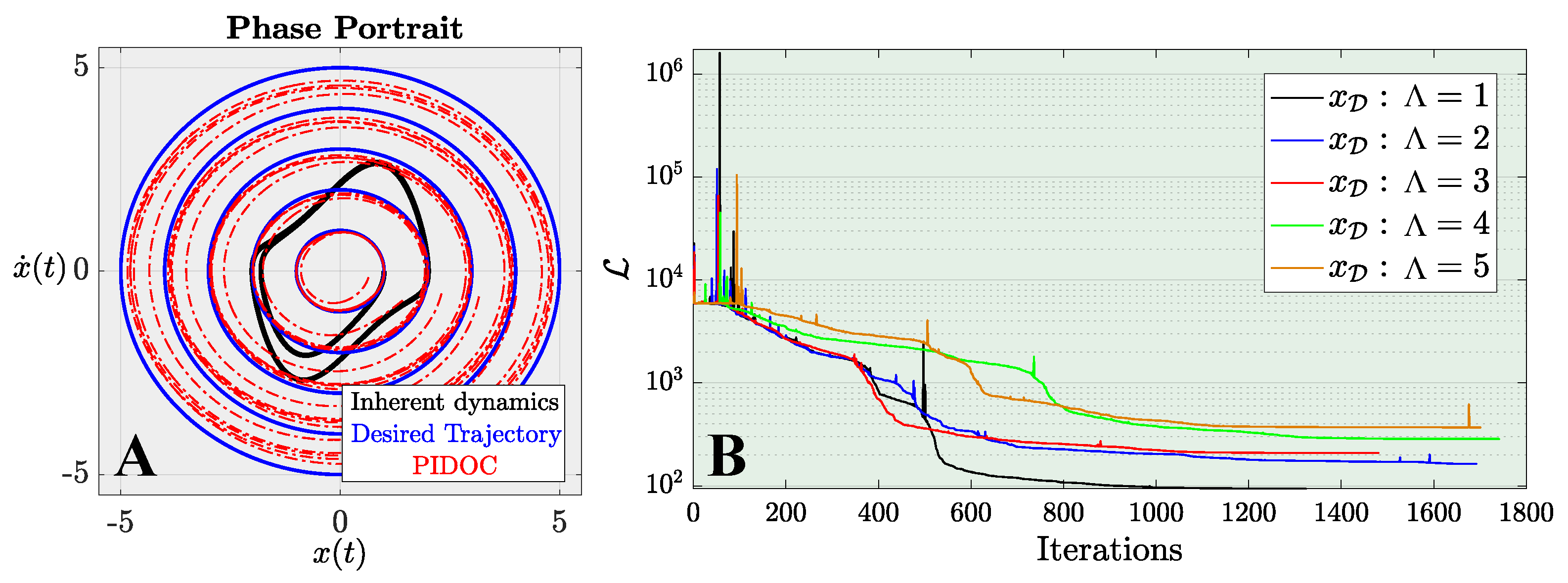
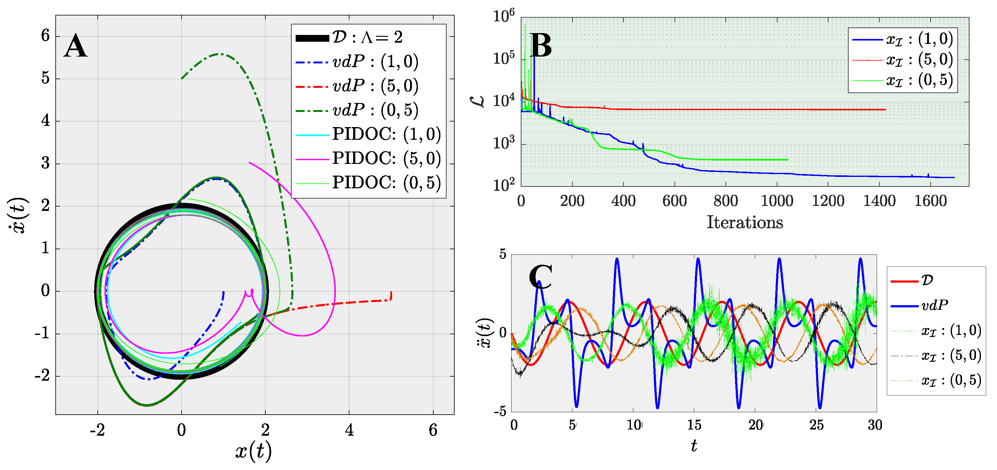
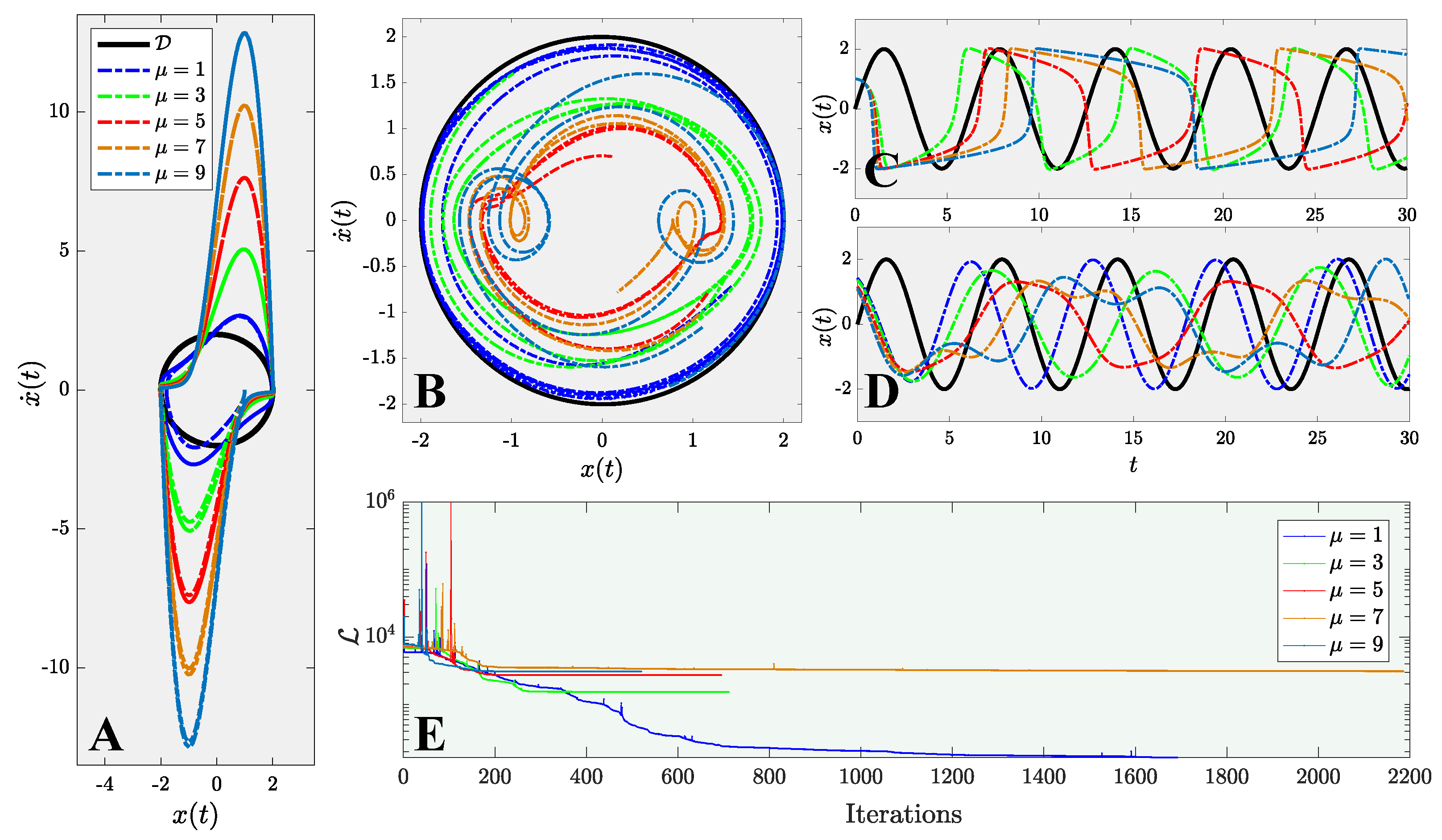
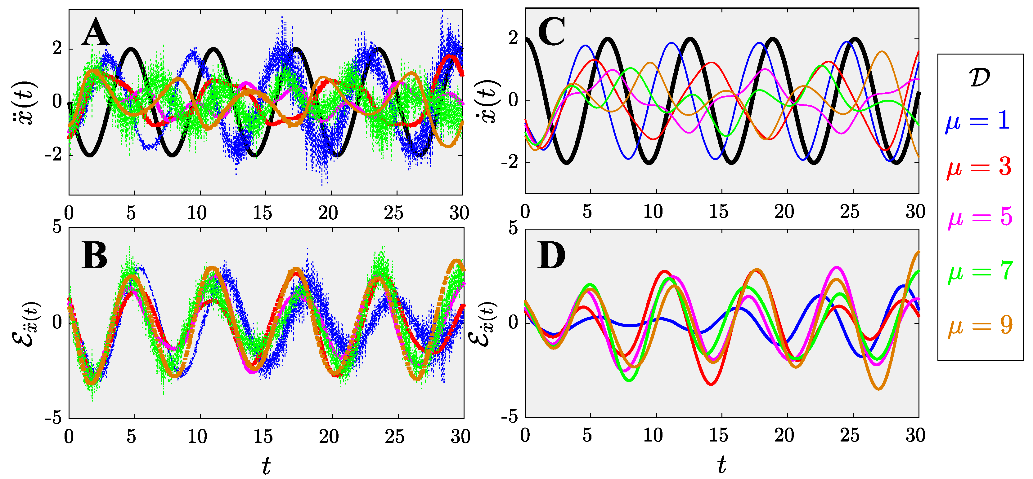
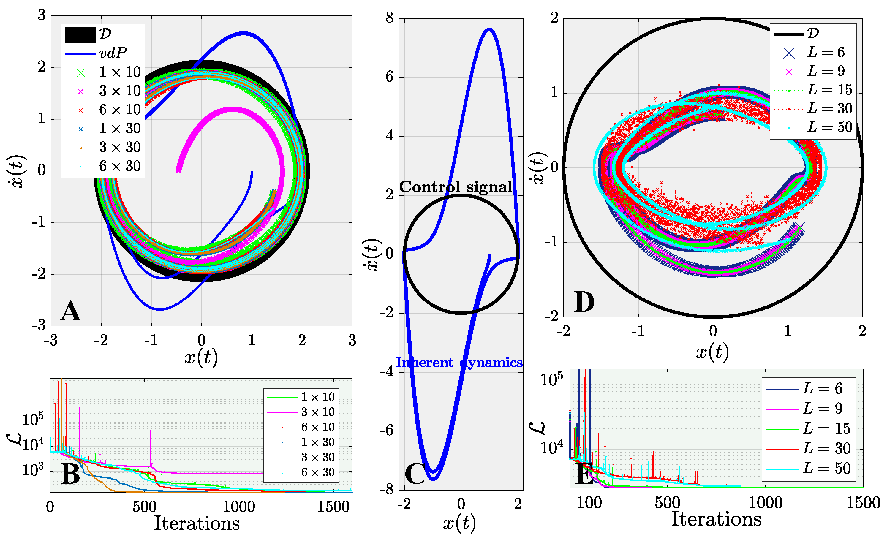
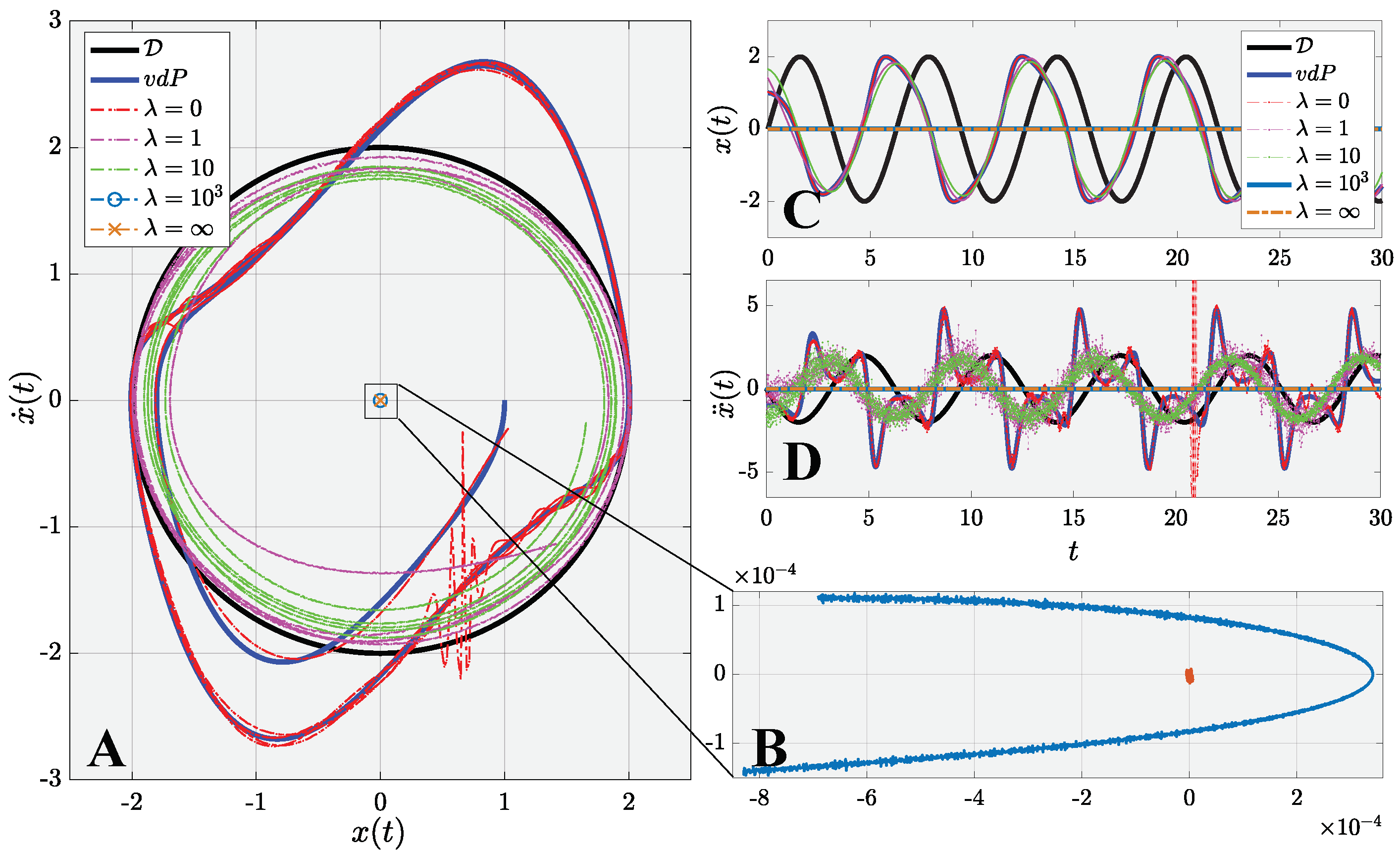
This manuscript describes a century-old yet widely encountered problem: controlling a nonlinear van der Pol dynamical system with a novel approach using physics-informed neural networks. Instead of adopting the traditional paradigm of learning and predicting using physics-informed neural networks, we use such networks for controlling nonlinear systems. A new framework based on physics-informed neural networks Physics-Informed Deep Operator Control (PIDOC) is presented, which consists of a deep neural network and physics-informed control, including the desired control trajectories and initial positions. PIDOC is fed with systematic nonlinear data to control the van der Pol circuits and output the controlled signals. To investigate the behavior and properties of PIDOC, we first tackled benchmark control problems for systematic analysis, then designed three sets of numerical experiments for testing the effects of the amplitudes of desired trajectories $\mathsf{\Lambda }$, different initial points $\mathcal{I}$, and system nonlinearities, as represented by $\mu$. We then tuned the hyper-parameters to change the neurons and layers of the neural network to study two questionss: (1) Does a neural network with a smaller volume still show the same capability for controls applied to the benchmark problem? (2) Can increasing the neural network volume lead to better capabilities with regard to controlling van der Pol systems with high nonlinearities? We also intended to verify the ability of single-hidden-layer neural networks to approximate nonlinear systems for part of the control. We also changed the Lagrange multiplier $\lambda$ to a weight factor to check how the desired trajectories guide PIDOC as control signals.

Our results indicate that PIDOC controls exhibit a higher stochasticity for higher-order terms, which can be attributed to the stochastic nature of deep learning, with the successful implementation of the desired trajectory on the benchmark problem. PIDOC also demonstrates the ability to increase the trajectory amplitudes with lower absolute mean errors. For systems with different initial points, our numerical experiments show that for points that are further away, PIDOC can still successfully implement controls with higher fluctuations at the initial stage. However, as we increase the system nonlinearities, the PIDOC outputs become less ideal than the benchmark problems, as two vortex-linked structures occur on the phase portrait, with an evidently higher loss observed for systems with high nonlinearities. A neural network with a decreased PIDOC volume also shows a good control implementation with the van der Pol system of $\mu =1$, while increasing the layers does not cause systems with high nonlinearity $\mu =5$ to follow the desired trajectory as well as the benchmark problem. It should be noted that increasing the layers does generate an improvement in the output-controlled signals, as the vortex-linked structures in phase portrait vanished, making the system more predictive. Increasing the weights of the control signals in PIDOC does not improve the control qualities based on the output. Even when the systematic data are nonlinear and chaotic, they still contribute greatly to the PIDOC, as the method is intrinsically a deep learning-based control method.

Considering the successful implementation of the van der Pol systems, further investigations on using PIDOC to impose control on other systems such as the Lorentz system could provide more insight. Additionally, a comparison of the control properties based on PIDOC and deterministic controls—i.e., Cooper et al. [47]—could also be a potential direct research. Specifically, comparing PIDOC with idealized nonlinear feedforward (open-loop), linearized feedback, and combined approaches could lead to unveiling more properties of PIDOC. Improvements in PIDOC or the development of further models tackling systems with high nonlinearities are significant goals to be addressed in future research.

References

1. Williams-Stuber, K.; Gharib, M. Transition from order to chaos in the wake of an airfoil. J. Fluid Mech. 1990, 213, 29–57. [Google Scholar] [CrossRef] [Green Version]
2. Argoul, F.; Arneodo, A.; Richetti, P.; Roux, J.C.; Swinney, H.L. Chemical chaos: From hints to confirmation. Acc. Chem. Res. 1987, 20, 436–442. [Google Scholar] [CrossRef]
3. Merali, Z. Robotic Roach Creates Order from Chaos. Available online: https://www.nature.com/articles/news.2010.15 (accessed on 1 December 2021).
4. Toker, D.; Sommer, F.T.; D’Esposito, M. A simple method for detecting chaos in nature. Commun. Biol. 2020, 3, 11. [Google Scholar] [CrossRef] [PubMed] [Green Version]
5. Błaz˙ejczyk, B.; Kapitaniak, T.; Wojewoda, J.; Brindley, J. Controlling Chaos in Mechanical Systems. Appl. Mech. Rev. 1993, 46, 385–391. [Google Scholar] [CrossRef]
6. Matsumoto, T. Chaos in electronic circuits. Proc. IEEE 1987, 75, 1033–1057. [Google Scholar] [CrossRef]
7. Lin, W.A.; Delos, J.B. Order and chaos in semiconductor microstructures. Chaos 1993, 3, 655–664. [Google Scholar] [CrossRef]
8. Mork, J.; Tromborg, B.; Mark, J. Chaos in semiconductor lasers with optical feedback: Theory and experiment. IEEE J. Quantum Electron. 1992, 28, 93–108. [Google Scholar] [CrossRef]
9. Chaos. Encyclopedia of Mathematics. Available online: http://encyclopediaofmath.org/index.php?title=Chaos&oldid=46308 (accessed on 1 December 2021).
10. González-Miranda, J.M. Synchronization and Control of Chaos: An Introduction for Scientists and Engineers; Imperial College Press: London, UK, 2004. [Google Scholar]
11. Lorenz, E.N. Deterministic non-periodic flow. J. Atmos. Sci. 1963, 20, 130–141. [Google Scholar] [CrossRef] [Green Version]
12. Ivancevic, V.G.; Ivancevic, T.T. Complex Nonlinearity: Chaos, Phase Transitions, Topology Change, and Path Integrals; Springer: Berlin/Heidelberg, Germany, 2008; ISBN 978-3-540-79356-4. [Google Scholar]
13. Safonov, L.A.; Tomer, E.; Strygin, V.V.; Ashkenazy, Y.; Havlin, S. Multifractal chaotic attractors in a system of delay-differential equations modeling road traffic. Chaos Interdiscip. J. Nonlinear Sci. 2002, 12, 1006–1014. [Google Scholar] [CrossRef]
14. Araki, M. PID Control. Available online: http://www.eolss.net/ebooks/Sample%20Chapters/C18/E6-43-03-03.pdf (accessed on 1 December 2021).
15. Bennett, S. A brief history of automatic control. IEEE Control. Syst. Mag. 1996, 16, 17–25. [Google Scholar] [CrossRef]
16. Slotine, J. Applied Nonlinear Control; Prantice-Hall: Englewood Cliffs, NJ, USA, 1991; Chapter 9. [Google Scholar]
17. Sung, S.W.; Lee, I.B. Limitations and Countermeasures of PID Controllers. Ind. Eng. Chem. Res. 1996, 35, 2596–2610. [Google Scholar] [CrossRef]
18. Mall, K.; Grant, M.J.; Taheri, E. Solving complex optimal control problems with nonlinear controls using trigonometric functions. Optim. Control. Appl. Methods 2021, 42, 616–628. [Google Scholar] [CrossRef]
19. Chen, L.; Chen, G. Fuzzy modeling, prediction, and control of uncertain chaotic systems based on time series. IEEE Trans. Circuits Syst. I Fundam. Theory Appl. 2000, 47, 1527–1531. [Google Scholar] [CrossRef]
20. Hassaan, M.; Elghandour, I. A Real-Time Big Data Analysis Framework on a CPU/GPU Heterogeneous Cluster: A Meteorological Application Case Study. In Proceedings of the 2016 IEEE/ACM 3rd International Conference on Big Data Computing Applications and Technologies (BDCAT), Shanghai, China, 6–9 December 2016; pp. 168–177. [Google Scholar]
21. LeCun, Y.; Bengio, Y.; Hinton, G. Deep learning. Nature 2015, 521, 436–444. [Google Scholar] [CrossRef]
22. Raissi, M.; Perdikaris, P.; Karniadakis, G.E. Physics-informed neural networks: A deep learning framework for solving forward and inverse problems involving nonlinear partial differential equations. J. Comput. Phys. 2019, 378, 686–707. [Google Scholar] [CrossRef]
23. Karniadakis, G.E.; Kevrekidis, I.G.; Lu, L.; Perdikaris, P.; Wang, S.; Yang, L. Physics-informed machine learning. Nat. Rev. Phys. 2021, 3, 422–440. [Google Scholar] [CrossRef]
24. Chen, Z.; Liu, Y.; Sun, H. Physics-informed learning of governing equations from scarce data. Nat. Commun. 2021, 12, 6136. [Google Scholar] [CrossRef]
25. Raissi, M.; Yazdani, A.; Karniadakis, G.E. Hidden fluid mechanics: Learning velocity and pressure fields from flow visualizations. Science 2020, 367, 1026–1030. [Google Scholar] [CrossRef]
26. Wang, R.; Kashinath, K.; Mustafa, M.; Albert, A.; Yu, R. Towards Physics-informed Deep Learning for Turbulent Flow Prediction. In Proceedings of the 26th ACM SIGKDD International Conference on Knowledge Discovery & Data Mining (KDD ’20), Virtual Event, CA, USA, 23–27 August 2020; pp. 1457–1466. [Google Scholar]
27. Pagnier, L.; Chertkov, M. Physics-Informed Graphical Neural Network for Parameter & State Estimations in Power Systems. arXiv 2021, arXiv:2102.06349. [Google Scholar]
28. Lee, J. Physics-Informed Neural Network for High Frequency Noise Performance in Quasi-Ballistic MOSFETs. Electronics 2021, 10, 2219. [Google Scholar] [CrossRef]
29. Choudhary, A.; Lindner, J.F.; Holliday, E.G.; Miller, S.T.; Sinha, S.; Ditto, W.L. Physics-enhanced neural networks learn order and chaos. Phys. Rev. E 2020, 101, 062207. [Google Scholar] [CrossRef] [PubMed]
30. Miller, S.T.; Lindner, J.F.; Choudhary, A.; Sinha, S.; Ditto, W.L. The scaling of physics-informed machine learning with data and dimensions. Chaos Solitons Fractals X 2020, 5, 100046. [Google Scholar] [CrossRef]
31. Raissi, M.; Perdikaris, P.; Karniadakis, G.E. Multistep Neural Networks for Data-driven Discovery of Nonlinear Dynamical Systems. arXiv 2018, arXiv:1801.01236. [Google Scholar]
32. Sun, F.; Liu, Y.; Sun, H. Physics-informed Spline Learning for Nonlinear Dynamics Discovery. In Proceedings of the Thirtieth International Joint Conference on Artificial Intelligence (IJCAI-21), Montreal, QC, Canada, 19–27 August 2021; Available online: https://www.ijcai.org/proceedings/2021/0283.pdf (accessed on 1 December 2021).
33. Antonelo, E.A.; Camponogara, E.; Seman, L.O.; de Souza, E.R.; Jordanou, J.P.; Hubner, J.F. Physics-Informed Neural Nets for Control of Dynamical Systems. arXiv 2021, arXiv:2104.02556. [Google Scholar]
34. Schiassi, E.; D’Ambrosio, A.; Drozd, K.; Curti, F.; Furfaro, R. Physics-Informed Neural Networks for Optimal Planar Orbit Transfers. J. Spacecr. Rocket. 2022, 1–16. [Google Scholar] [CrossRef]
35. Hagan, M.T.; Demuth, H.B. Neural networks for control. In Proceedings of the 1999 American Control Conference (Cat. No. 99CH36251), San Diego, CA, USA, 2–4 June 1999; Volume 3, pp. 1642–1656. [Google Scholar] [CrossRef]
36. Nguyen, D.H.; Widrow, B. Neural networks for self-learning control systems. IEEE Control. Syst. Mag. 1990, 10, 18–23. [Google Scholar] [CrossRef]
37. Antsaklis, P.J. Neural Networks in Control Systems. IEEE Trans. Neural Netw. 1990, 1, 242–244. [Google Scholar] [CrossRef]
38. Van der Pol, B. On “Relaxation Oscillations” I. Philos. Mag. 1926, 2, 978–992. [Google Scholar] [CrossRef]
39. Van der Pol, B. The nonlinear theory of electric oscillations. Proc. IRE 1934, 22, 1051–1086. [Google Scholar] [CrossRef]
40. Van der Pol, B.; van der Mark, J. Frequency de-multiplication. Nature 1927, 120, 363–364. [Google Scholar] [CrossRef]
41. Novak, T. Design principles of biochemical oscillators. Nat. Rev. 2008, 9, 981–991. [Google Scholar] [CrossRef] [PubMed] [Green Version]
42. Rompala, K.; Rand, R.; Howland, H. Dynamics of three coupled van der Pol oscillators with application to circadian rhythms. Commun. Nonlinear Sci. Numer. Simul. 2007, 12, 794–803. [Google Scholar] [CrossRef] [Green Version]
43. Kaplan, B.Z.; Gabay, I.; Sarafian, G.; Sarafian, D. Biological applications of the “Filtered” Van der Pol oscillator. J. Frankl. Inst. 2008, 345, 226–232. [Google Scholar] [CrossRef]
44. Chagas, T.P.; Toledo, B.A.; Rempel, E.L.; Chian, A.C.-L.; Valdivia, J.A. Optimal feedback control of the forced van der Pol system. Chaos Solitons Fractals 2012, 45, 1147–1156. [Google Scholar] [CrossRef]
45. Sayed, M.; Elagan, S.K.; Higazy, M.; Abd Elgafoor, M.S. Feedback Control and Stability of the Van der Pol Equation Subjected to External and Parametric Excitation Forces. Int. J. Appl. Eng. Res. 2018, 13, 3772–3783. [Google Scholar]
46. Batool, A.; Hanif, A.; Hamayun, M.T.; Ali, S.M.N. Control design for the compensation of limit cycles in Van Der Pol oscillator. In Proceedings of the 2017 13th International Conference on Emerging Technologies (ICET), Islamabad, Pakistan, 27–28 December 2017; pp. 1–6. [Google Scholar] [CrossRef]
47. Cooper, M.; Heidlauf, P.; Sands, T. Controlling Chaos—Forced van der Pol Equation. Mathematics 2017, 5, 70. [Google Scholar] [CrossRef] [Green Version]
48. Duke University. The van der Pol System. Available online: https://services.math.duke.edu/education/ccp/materials/diffeq/vander/vand1.html (accessed on 1 December 2021).
49. Dogruer, T.; Tan, N. Design of PI Controller using Optimization Method in Fractional Order Control Systems. IFAC-PapersOnLine 2018, 51, 841–846. [Google Scholar] [CrossRef]
50. Zhai, H.; Zhou, Q.; Hu, G. BubbleNet: Inferring micro-bubble dynamics with semi-physics-informed deep learning. arXiv 2021, arXiv:2105.07179. [Google Scholar]
51. Schult, D. Math 329—Numerical Analysis Webpage. Available online: http://math.colgate.edu/math329/exampleode.py (accessed on 1 December 2021).
52. Mulansky, M.; Ahnert, K. Odeint library. Scholarpedia 2014, 9, 32342. [Google Scholar] [CrossRef]
53. Müller-Komorowska, D. Differential Equations with SciPy—Odeint or Solve_ivp. Scientific Programming Blog. Available online: https://danielmuellerkomorowska.com/2021/02/16/differential-equations-with-scipy-odeint-or-solve_ivp/ (accessed on 1 December 2021).
54. Lu, L.; Meng, X.; Mao, Z.; Karniadakis, G.E. DeepXDE: A Deep Learning Library for Solving Differential Equations. SIAM Rev. 2021, 63, 208–228. [Google Scholar] [CrossRef]
55. Liu, D.C.; Nocedal, J. On the limited memory BFGS method for large scale optimization. Math. Program. 1989, 45, 503–528. [Google Scholar] [CrossRef] [Green Version]
56. Abadi, M.; Agarwal, A.; Barham, P.; Brevdo, E.; Chen, Z.; Citro, C.; Corrado, G.S.; Davis, A.; Dean, J.; Devin, M.; et al. TensorFlow: Large-Scale Machine Learning on Heterogeneous Systems, 2015. Available online: tensorflow.org (accessed on 1 December 2021).
57. Asl, A. Behavior of the Limited-Memory BFGS Method on Nonsmooth Optimization Problems in Theory and Practice. Ph.D. Thesis, New York University, New York, NY, USA, 2020. Available online: https://cs.nyu.edu/media/publications/asl_thesis_final_UtpoLsu.pdf (accessed on 1 December 2021).
58. Kazmierkowski, M.P.; Malinowski, M.; Beach, M. CHAPTER 4—Pulse Width Modulation Techniques for Three-Phase Voltage Source Converters. In Control in Power Electronics; Academic Press: Cambridge, MA, USA, 2002; pp. 89–160. [Google Scholar] [CrossRef]
59. Bisong, E. Google Colaboratory. In Building Machine Learning and Deep Learning Models on Google Cloud Platform; Apress: Berkeley, CA, USA, 2019. [Google Scholar] [CrossRef]
60. Ramos, A. Automatic differentiation for error analysis of Monte Carlo data. Comput. Phys. Commun. 2019, 238, 19–35. [Google Scholar] [CrossRef] [Green Version]
61. Pinkus, A. Approximation theory of the MLP model in neural networks. Acta Numer. 1999, 8, 143–195. [Google Scholar] [CrossRef]
Figure 1. The schematic diagram for the van der Pol circuits. Note that the nonlinearity originating from the semiconductor (the green part) causes the system to generate chaotic behavior. The cycle of the oscillating circuits generates current, as illustrated by the dashed circle. See text for details.
Mathematics 10 00453 g001
Figure 2. The phase portrait for the nonlinear van der Pol equation when μ = 1 . The phase is initiated from six different points: ( 1 , 0 ) , ( 2 , 0 ) , ( 3 , 0 ) , ( 0 , 1 ) , ( 0 , 2 ) , ( 0 , 3 ) . As indicated in the different dashed lines in the box, both converge to the same nonlinear trajectory of the van der Pol inherent dynamics. Note that the data for this figure were generated using odeint in SciPy library.
Mathematics 10 00453 g002
Figure 3. The schematic diagram for the Physics-Informed Deep Operator Control framework inspired by PINN. The system data of the nonlinear van der Pol oscillator are input to the deep learning framework, as automatic differentiation can encode physics information as in the purple box. The encoded information is further forwarded to the loss function, as the Langrangian multiplier λ can enlarge the control signal, which provides feedback to the deep learning scheme for learning the dynamics and can thereby output the ideal dynamics.
Mathematics 10 00453 g003
Figure 4. The system behavior of the use of PIDOC to control the van der Pol dynamics applied to the benchmark problem. (A) the phase portrait of the desired trajectory D , the PIDOC-controlled signal, and the van der Pol inherent dynamics. (B) Plot of position x ( t ) against time t. (C) Plot of acceleration x ¨ ( t ) against time t.
Mathematics 10 00453 g004
Figure 5. Systematic behavior analysis of PIDOC applied to different trajectory amplitudes Λ . (A) The phase portrait of the inherent dynamics, with five different desired trajectories Λ = 1 , 2 , , 5 marked in blue solid lines and the corresponding PIDOC-controlled outputs marked in red dotted lines. (B) the loss function–iteration diagram for the five trajectories.
Mathematics 10 00453 g005
Figure 6. Systematic behavior estimation of PIDOC applied to the control signals Λ = 2 with different initial positions. Note that D and v d P in the plot legend stand for the desired trajectory and van der Pol inherent dynamics. (A) Phase portrait of the desired trajectory; inherent dynamics given three different initial points: ( 1 , 0 ) , ( 5 , 0 ) , and ( 0 , 5 ) ; and PIDOC-controlled trajectories given three initial positions. (B) The loss function–iteration diagram is given three different initial points. (C) The acceleration x ¨ ( t ) –time plot of the desired trajectory D , van der Pol inherent dynamics, and the three PIDOC-controlled routes given different initial positions.
Mathematics 10 00453 g006
Figure 7. System analysis of PIDOC considering the nonlinearity of the van der Pol systems with different μ . (A) The inherent dynamics of different van der Pol systems with different μ marked in dashed lines with different colors, with the desired control trajectory D marked in black. (B) The phase portrait of the desired trajectory corresponding to PIDOC applied to different systems of different nonlinearities. (C) The position plot showing the time t of the system’s inherent dynamics. (D) The position plot with time t of the PIDOC controlled dynamics. (E) the loss function—iterations plot of PIDOC applied to van der Pol systems of different nonlinearities. Note that the colors used for different PIDOC controls of different nonlinearities all correspond to subfigure (A).
Mathematics 10 00453 g007
Figure 8. The plot of velocity x ˙ ( t ) and acceleration x ¨ ( t ) and their corresponding errors regarding time t and considering cases of different nonlinearities. Note that the colors used for cases in van der Pol systems of different nonlinearities are shown in the legend on the right side, where D stands for the desired control trajectory. (A) The acceleration x ¨ ( t ) -t diagram. (B) The errors in the acceleration. (C) The acceleration x ˙ ( t ) -t diagram. (D) the errors in the velocity.
Mathematics 10 00453 g008
Figure 9. System behavior analysis of how the neural network structure tunes the control process of PIDOC for μ = 1 and μ = 5 . (A) the phase portrait of PIDOC controls considering different neural network structures; the solid black line D denotes the desired trajectory, the blue solid line v d P denotes the van der Pol inherent dynamics. Different colored cross dots, as marked in the legend, denote different neural network structures. Note that subfigures (A,B) share the same color representation of the neural network structure. (B) The loss function–iteration diagram for different neural network structures as applied to the benchmark problem of μ = 1 . (C) The inherent van der Pol dynamics (marked as a blue solid line) when μ = 5 . (D) The phase portrait of PIDOC applied to highly nonlinear van der Pol system of μ = 5 corresponds to subfigure (C). Note that the black solid line D is the desired trajectory. Different neural network structures are denoted by cross dots in different colors, as indicated in the legend. (E) The loss function–iteration diagram corresponds to subfigure (D).
Mathematics 10 00453 g009
Figure 10. System behavior analysis of the effects of the Lagrange multiplier on the control signal implementation for PIDOC. Note that the black solid line D is the desired trajectory, the blue solid line v d P denotes the van der Pol inherent dynamics, and the controlled routes of different Lagrange multiplier values are denoted in differently colored dashed lines. Note that all the colors in the subfigures are marked the same as those represented in the legend in subfigure (A). (A) The phase portrait of the PIDOC controls. (B) Zoomed view of rescaled Lagrange multipliers λ = 10 3 and λ = . (C) The position x ( t ) against time t for the desired trajectory D , van der Pol inherent dynamics, and different PIDOC controls. (D) The acceleration x ¨ ( t ) against time t for the desired trajectory D , van der Pol inherent dynamics, and different PIDOC controls.
Mathematics 10 00453 g010