Article

Early Prediction of DNN Activation Using Hierarchical Computations

by
Bharathwaj Suresh
1,*,
Kamlesh Pillai
1,*,
Gurpreet Singh Kalsi
1,
Avishaii Abuhatzera
2 and
Sreenivas Subramoney
1
1
Processor Architecture Research (PAR) Lab, Intel Labs, Bangalore 560048, India
2
Corporate Strategy Office, Intel, Haifa 3508409, Israel
*
Authors to whom correspondence should be addressed.
Mathematics 2021, 9(23), 3130; https://doi.org/10.3390/math9233130
Submission received: 11 October 2021 / Revised: 30 November 2021 / Accepted: 1 December 2021 / Published: 4 December 2021
(This article belongs to the Special Issue Computational Optimizations for Machine Learning)

Abstract

:
Deep Neural Networks (DNNs) have set state-of-the-art performance numbers in diverse fields of electronics (computer vision, voice recognition), biology, bioinformatics, etc. However, the process of learning (training) from the data and application of the learnt information (inference) process requires huge computational resources. Approximate computing is a common method to reduce computation cost, but it introduces loss in task accuracy, which limits their application. Using an inherent property of Rectified Linear Unit (ReLU), a popular activation function, we propose a mathematical model to perform MAC operation using reduced precision for predicting negative values early. We also propose a method to perform hierarchical computation to achieve the same results as IEEE754 full precision compute. Applying this method on ResNet50 and VGG16 shows that up to 80% of ReLU zeros (which is 50% of all ReLU outputs) can be predicted and detected early by using just 3 out of 23 mantissa bits. This method is equally applicable to other floating-point representations.

1. Introduction

Ever since its inception, deep learning has evolved into one of the most widely used technique to solve problems in the area of speech recognition [1], pattern recognition [2], and natural language processing [1]. The effectiveness of Deep Neural Networks (DNNs) is pronounced when there is a huge amount of data with minimal features which are not easily apparent to humans [2]. This makes DNNs valuable tools to meet future data processing needs. However, producing accurate results using a large dataset comes at a cost. DNN inference requires a huge amount of computing power, and, as a result, consumes a large amount of energy. In a study by Strubell et al., it was estimated that training a single deep learning model can emit the same amount of CO2 as five cars do throughout their lifetime [3]. Due to this fact, optimizing DNN implementations has become an urgent requirement, and has been receiving widespread attention from the research community [4,5,6].
In their basic form, DNNs consist of simple mathematical operations like addition and multiplication, which are combined together to form the multiply and accumulate (MAC) operation. In fact, up to 95% of the computational workload of a DNN is due to MAC operations [7]. In a typical DNN, about a billion MAC operations are required to process each input sample [8]. This fact suggests that improving the efficiency of the MAC operations would contribute significantly towards reducing the computational requirement of DNNs. One way to do this is to reduce the number of bits used to perform the MAC operations, an idea that has been widely explored in the field of approximate computing [9]. Some studies have shown that using approximate computing techniques for DNN implementation can reduce power consumption by as much as 88% [10]. However, the majority of the approximate computing techniques result in a decrease of accuracy, which may not be acceptable for some applications. In particular, the training of DNNs, which could take many days even using GPUs, require high-precision floating-point values to achieve best results [11]. Hence, it is important to come up with methods that can make computation of DNNs more efficient without reducing the accuracy of the output.
A typical DNN consists of many convolution and fully connected layers. Each of these layers perform MAC operation on the input using weights that are trained to generate a unique feature representation as the output [1]. Many such layers placed in succession can be used to approximate a target function. While the convolution and fully-connected layers alone are sufficient to represent linear functions, they cannot be used directly for applications that need nonlinear representations. To introduce nonlinearity into the model, the outputs of the convolution and fully-connected layers are passed through a nonlinear operator called an activation function [12]. As every output value is required to pass through an activation function, choosing the right activation function is an important factor for the effectiveness of DNNs [13].
One of the most widely used activation function is the Rectified Linear Unit (ReLU) [14]. The simple, piece-wise linear nature of ReLU can enable faster learning, and maintain stable values when using gradient-descent methods [12]. The output of a ReLU function is the same as the input when the input is positive, and is zero for negative inputs. This means that the precision of output is important only when the input is a positive value. Input to a ReLU function is usually the output from a fully-connected or convolution layer of the DNN which consist of a large number of MAC operations [8]. Studies have found that between 50% to 95% of ReLU outputs in DNNs are zero [15]. Hence, a lot of high precision compute in DNNs is wasted where output elements are reduced to zero after ReLU function. Early detection of these negative values can result in reducing the energy spent on high precision MAC operations, which would ultimately result in an efficient DNN implementation.
To this end, our work proposes a method for early detection of negative input values to the ReLU function, accounting for the maximum possible error while performing MAC with reduced precision. Using these values, we develop a mathematical model that provides a threshold below which a negative output value is guaranteed, irrespective of the remaining bits to be computed. It is shown that a proposed model can detect up to 80% negative values for popular CNN models using just three mantissa bits of floating-point number. This mathematical model can be used as the basis to implement low-precision MAC operations for DNNs adopting ReLU functions, which would result in efficient DNN implementation without a loss in accuracy. In summary, our contributions are threefold:
  • Study of the fraction of ReLU zeros in two popular CNN models—VGG16 [16] and ResNet50 [17].
  • A mathematical model that can accurately detect negative values based on the number of mantissa bits used a low precision MAC operation.
  • Implementation of the developed model to detect ReLU zeros early in the VGG16 [16] and ResNet50 [17] inference stage.

2. Literature Review

The training and inference of DNNs is a compute intensive task, and has resulted in the need for various hardware accelerators [18,19,20,21,22,23]. Memory performance can be optimized through data locality by maximizing the reuse of data at buffers close to the compute block, as shown by Chen et al. [20]. A bit serial approach was considered by Judd et al. to reduce overall computations required by reducing activation precision [21]. Unnecessary multiplication with zero values was eliminated in Cnvlutin, which resulted in improved performance [19]. TETRIS used a high bandwidth 3D memory, which lead to reduced internal buffer size, for dealing with the memory bottleneck issue and overcoming the memory bottleneck [23]. Pruning techniques have also been studied to maximize compute saving by exploiting the sparsity in DNNs [24]. However, these methods are typically used for very specific applications and are expensive to generalize.
Approximate computing has emerged as one of the most effective solutions for generic DNNs, and it can exploit the inherent resilience of the CNN model (i.e., its ability to handle variations in data and still be able to figure out the pattern) and reduce the computation costs [25]. The level of approximation could be varied for different DNN models and datasets, hence approximate computing gained popularity [9]. This has led many researchers to investigate methods to perform low-precision computations in DNNs [26,27,28,29,30,31,32,33].
One of the most commonly applied technique is quantization, which is the process of replacing floating point numbers by numbers with reduced bit width. A study by Gupta et al. [26] demonstrated DNN training using 16-bit wide floating-point number with a very small reduction in accuracy as compared to a 32-bit floating-point number. Another study explored the effect of variable precision across different CNN layers, and demonstrated accuracy close to the benchmarks [27]. Venkatesh et al. studied the possibility of using 2-bit weights and space computing methods to produce state-of-the-art results. The study employed few iterations of full-precision training, followed by reduced precision training and inference [30]. The study on compute complexity is reduction using a 1D kernel factorized network is presented in the work [34].
Another approach in approximate computing is the use of multipliers and adders that compute results in a simplified manner. The work by Sarwar et al. [29] highlighted the use of simplified add and shift operations for power savings in DNNs. Another study explored the use of alternate full-adder implementation for efficient CNN hardware [28]. Stochastic computing based circuits have also been studied as potential candidates to implement a low-power DNN hardware accelerator [32].
Approximate computing has also been pursued at the software level, by simplifying the DNN architectures to reduce compute. Pruning the synaptic weights, reducing bit width of the synapse, and minimizing the number of hidden layers or neurons within these layers were demonstrated as effective methods to develop energy efficient DNNs [29]. Wei et al. came up with a more structured approach with pattern-based weight pruning for real-time DNN execution [33].
While all these studies have highlighted the relevance and requirement of approximate computing, they also mentioned that it comes at the cost of reduced accuracy. However, DNNs often require high precision floating point values during training to achieve high accuracy and reduced training time [35,36,37]. Such a reduction in accuracy may be unacceptable in real-life applications like self-driving cars [38] or medical diagnosis [39,40], where errors could be life threatening. Hence, most commercial DNNs still use floating point precision in their computations [41,42]. Hence, it is important to come up with a method to perform low precision computations in DNNs without reducing the accuracy of the model.
Shormann et al. proposed a method to reduce convolution operations in CNNs by dynamically predicting zero-valued outputs [43]. SnaPEA performs a reordering of weights and keeps track of the partial sum to predict zero outputs early [44]. A similar method was employed by Asadikouhanjani et al. to propose an efficient DNN accelerator [45]. By considering the spatial surroundings of an output feature map, Mosaic-CNN performs reduced precision compute to predict zero values early [46]. Other studies have explored methods to predict the zero values in an output feature map using the sign values [47,48,49]. Our study attempts further research in this direction by proposing a novel method to predict ReLU zeros with reduced precision compute.

3. Background

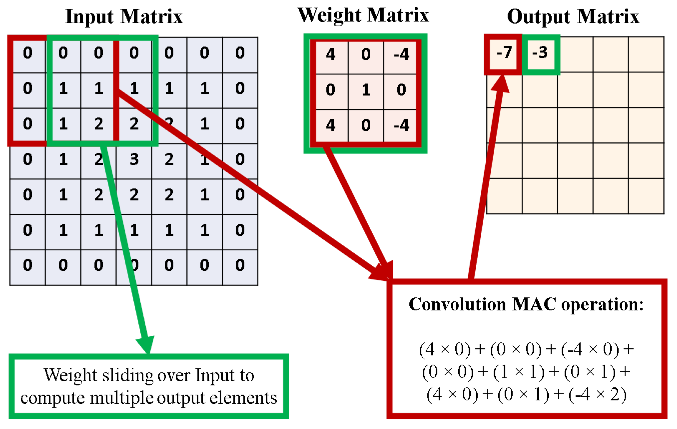
3.1. Convolutional Neural Networks

Among the different types of DNNs, Convolutional Neural Networks (CNNs) are extensively used in image processing, computer vision, and speech processing applications, often resulting in superior performance [50]. The convolution layer, which converts the input image into a form that is easier to process by the next layer, is at the heart of a CNN. Convolution is the application of a filter to an input to produce an output feature map to indicate a detected feature in the input data. Both the input values and the filter values are represented as matrices, with the filter dimensions typically being much smaller that the input. The values in the filter matrix are multiplied with the corresponding values in the input matrix, and the values are added to produce a single output value. This MAC operation is repeated by shifting the filter by a fixed amount each time, resulting in an output feature map. The number of element shifts by the weight matrix on the input matrix is called the stride. This convolution process is demonstrated in Figure 1. As shown in Figure 1, each term from the input layer is multiplied with every term in the filter matrix, and these values are added together (accumulate) to generate one value in the output feature map. This process is repeated by moving the filter matrix across the input matrix, until it has been traversed completely. Once the output feature map is generated, it is passed through an activation function (like ReLU) to introduce nonlinearity.

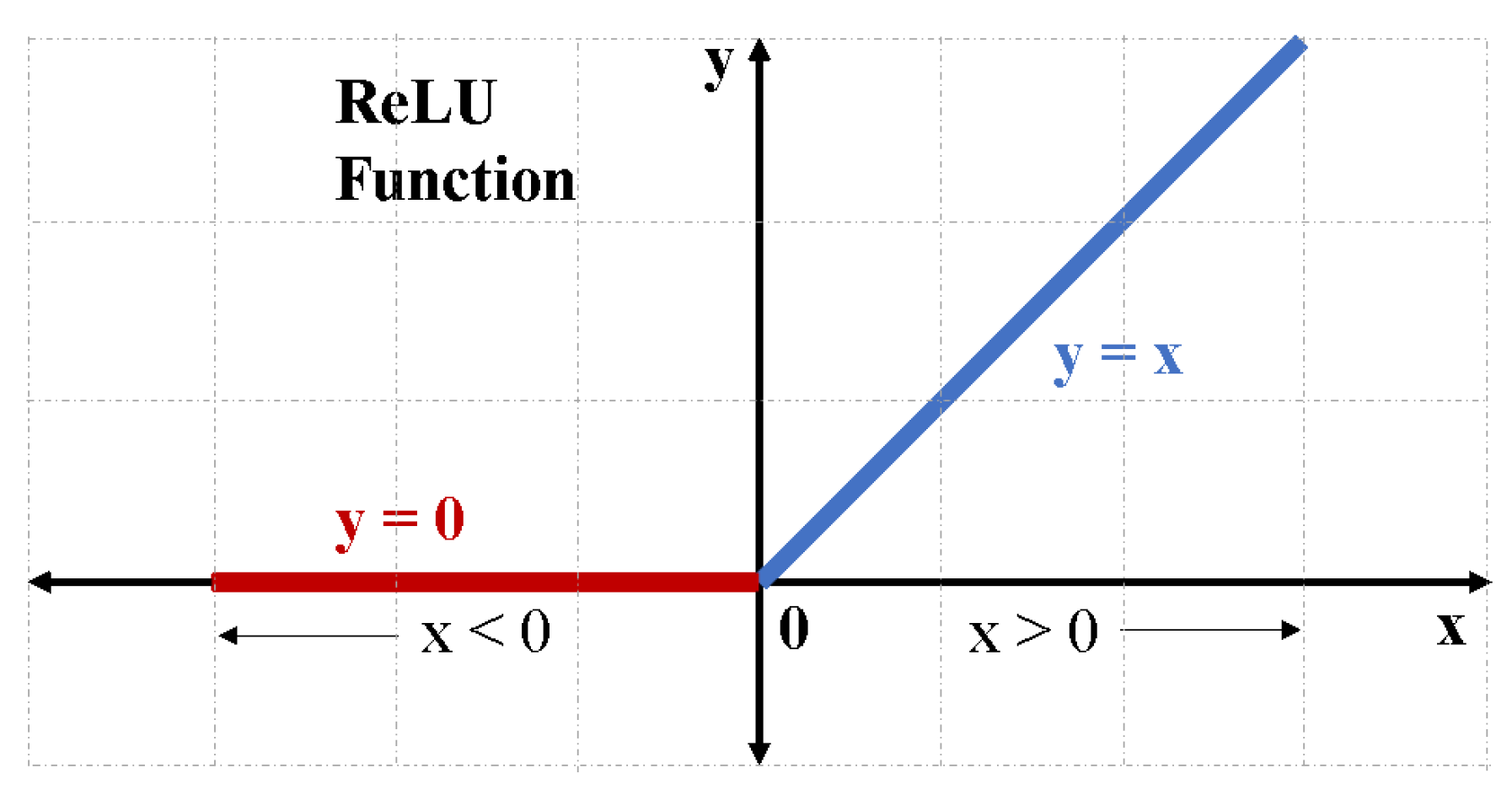
3.2. ReLU Activation Function

The ReLU activation function is one of the most popular activation functions used in DNNs today [14]. The function returns zero for all negative inputs, and returns the input if it is a non-negative value. It can be written as:
f ( x ) = m a x ( 0 , x )
where max returns larger of the two inputs. The graphical representation is shown in Figure 2. The success of ReLU can be attributed to its simple implementation, which in turn reduces the computation time of the DNN model [51]. In addition, a majority of the ReLU outputs are zero [15], which makes the output matrix sparse and results in better prediction and reduced chances of overfitting [52]. Both the ReLU function and its derivative are monotonic, which ensures that the vanishing gradient problem is avoided when the gradient-descent training process is employed [53]. These factors have contributed to the widespread use of ReLU activation function in DNNs. Hence, the study of the ReLU activation function is important to implement DNNs more efficiently.

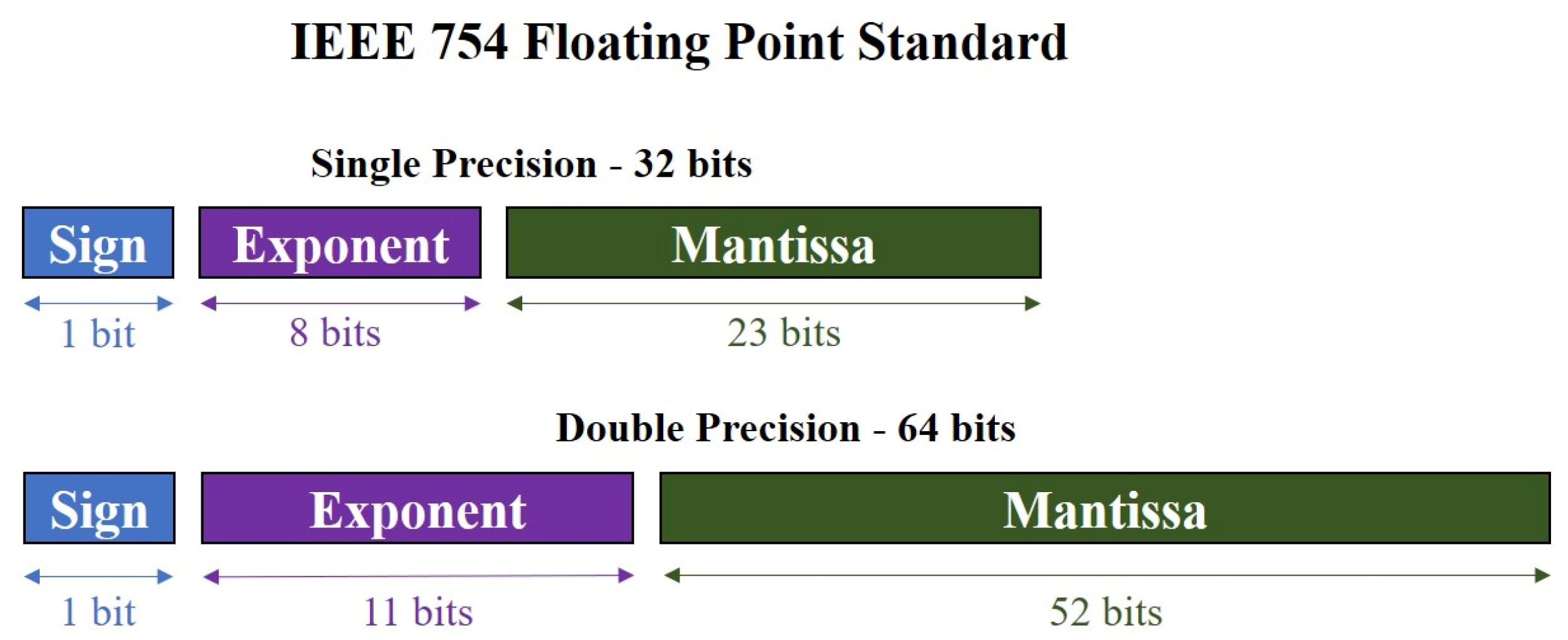
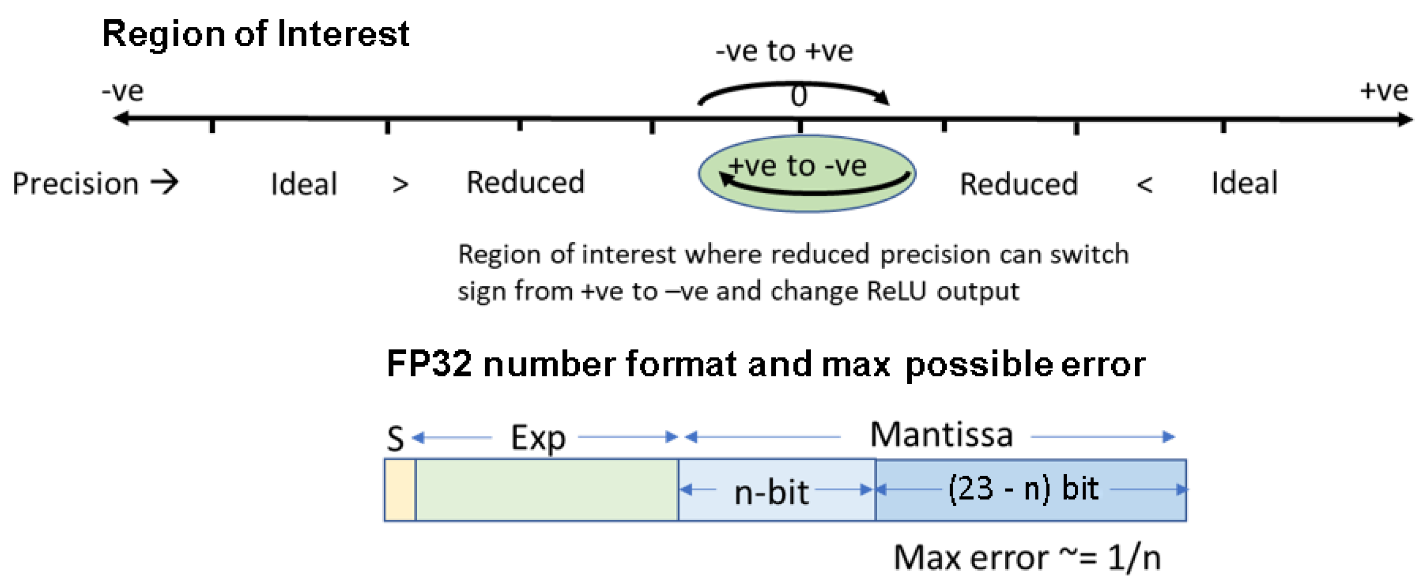
3.3. Floating Point Number Representation

In any typical DNN, the input, output, and intermediate values are stored in the floating-point format. The standard format used in a majority of applications is the IEEE-754 floating point number format [54]. In this format, the Most Significant Bit (MSB) is the Sign bit (S) which is 0 for positive numbers, and 1 for negative numbers. This is followed by a fixed number of bits assigned to store the Exponent E, and the remaining bits are allotted to the Mantissa M. The fractional part is stored in the normalized form—i.e., the actual values in binary is 1 plus the fractional value represented by M. In order to accommodate negative exponent values, 127 is added (called excess-127). Hence, the actual exponent is E–127. Based on these rules, the floating point value represented using the S, E and M values in the IEEE-754 format is:
F = ( 1 ) S × 2 ( E 127 ) × ( 1 + M )
The two commonly used forms of the IEEE-754 format are the single and double precision format. In the single precision representation, there are 8 exponent bits and 23 mantissa bits to make a total of 32 bits. The double precision is a 64-bit representation with 11 exponents and 52 mantissa bits [54]. Figure 3 graphically depicts both the single and double precision representations.

4. Methodology

4.1. Dataset and Framework

As image recognition is one of the most widely used and researched applications of CNNs, we focus our analysis on models within this domain. VGG-16 is one of the pioneer CNN models for large scale image recognition tasks [16]. It takes a 224 × 224 RGB image as input and passes it through different convolution, max-pooling, and fully connected layers. The final classification is implemented using a softmax layer. Figure 4 describes the VGG-16 architecture. As evident from the figure, there are 13 convolution layers, and each convolution layer is followed by a ReLU activation layer. A set of convolution layers are followed by pooling layers to reduce the dimensions of the input before sending it to the next convolution sets. Finally, a set of fully-connected layers are added to produce the output classification probability.
As DNNs like VGG16 became difficult to train, Residual Networks (ResNets) emerged as improved alternatives. In ResNets, shortcut (or identity) connections were introduced between different layers to perform quick identity mapping with no additional model parameters [17]. One such ResNet model is the ResNet-50, which has 50 different convolution and fully-connected layers along the path from input to output. Like VGG-16, ResNet-50 also takes 224 × 224 RGB images as its input. The ResNet50 architecture is shown in Figure 5. A convolution operation that is applied on the input and the layer size is reduced before it is sent to the residual layers. Each of the residual layers is comprised of three sets, each with a convolution layer followed by a ReLU activation layer. Before the last ReLU operation, an identity connection is added to train identity mappings in some of the layers. The Res 2–1, Res 3–1, and Res 4–1 groups shown in Figure 5 have a convolution layer in the identity path. These residual layers are followed by a pooling and fully-connected layer, which give the classification probabilities as the output.
These models were tested using the ImageNet Large Scale Visual Recognition Challenge 2012 (ILSVRC2012) inference dataset, which includes 50,000 images belonging to 1000 different classes [55]. These images were converted to the 224 × 224 RGB format, and the pixel values were normalized. To ensure that the training methods were standard, the pretrained models of ResNet-50 and VGG-16 were used from the Keras library [56] running on top of the TensorFlow [57] backend.

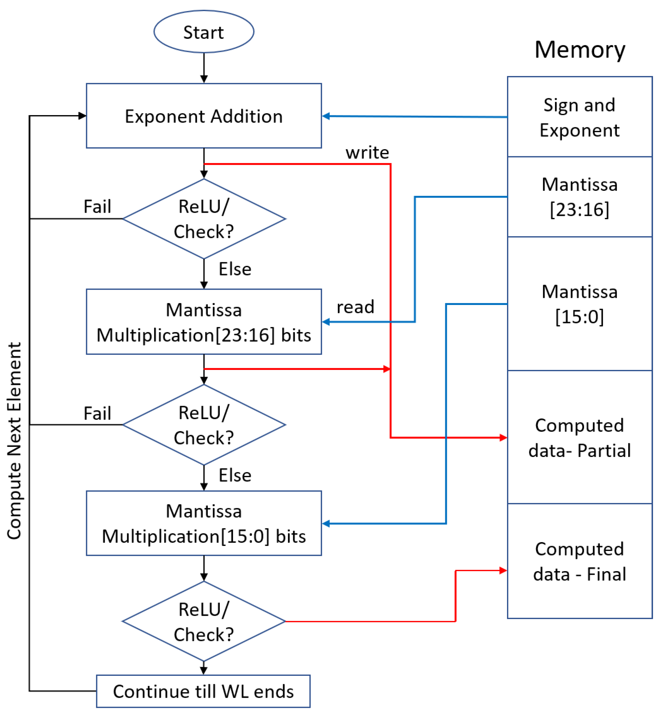
4.2. Proposed Hierarchical Computation

It is evident that each convolution layer involves MAC operations between the input values and a filter with the trained weight values. The result of this MAC operation is passed through the ReLU activation function and negative values are made zero. Our implementation includes an intermediate step that predicts negative values early using a reduced number of mantissa bits. The MAC operation is performed using reduced mantissa bits, and the output is obtained. Then, based on the number of mantissa bits used for the computation, the proposed model predicts whether a value estimated is definitely negative or not. If the value is determined to be negative, the output is made to be zero. For the other values, we perform MAC using the full precision and obtain the output like in typical implementations. Hence, we reduce the total number of cases for which the expensive full precision compute must be performed, while simultaneously ensuring no loss in accuracy.
The steps are described using a flowchart in Figure 6. In the case presented, for every workload, we first perform computation without any mantissa bits. Since only exponent values are present, this can be achieved directly by adding the exponent bits. If output can be predicted to be negative at this step, then set the output as zero and move on to the next set of element of the input workload. If inconclusive, the first 8 MSB mantissa bits (bits 23 to 16) are considered for further computation. Once again, predict the accumulated negative value, and set those outputs to zero. For cases where the accumulated element sign is still ambiguous, the remaining mantissa bits (bits 15 to 0) are also used and the full precision compute is performed. The remaining outputs are obtained after this step, and this whole cycle is repeated for the other input workloads. This way, the total compute can be split into multiple levels by adding additional mantissa bits. At each level, some negative values can be detected with reduced precision compute. At the same time, full precision compute can be performed for all positive outputs, ensuring no loss in accuracy. The selection of levels of compute and bits selection for each level can be determined based on model, workload, and underlying compute hardware availability. The impact of selected mantissa bits on correctly predicted negative values is described later in the Results section.
Figure 7 intuitively describes the proposed hierarchical computation approach to estimate ReLU output with reduced precision compute. Here, the “Ideal” is the value that is computed with full precision, while “Reduced” is the output with only a few MSB mantissa bits considered. If “Reduced” is a large negative value, the output can be estimated to be negative irrespective of the mantissa bits. Our model detects such values until it reaches a threshold, where “Reduced” is negative but close to zero. To estimate these values correctly, more mantissa bits (next set of MSB bits) need to be considered. Similarly, when “Reduced” is a large positive value, it can be estimated to be positive without using the mantissa bits. However, as the value approaches zero, more mantissa bits are required to correctly estimate the sign of the element. A threshold is estimated along the positive axis too, beyond which values are always positive. Our model determines both the positive and negative thresholds, which gives rise to the region of interest where full precision compute needs to be performed, as shown in Figure 7. These thresholds are obtained by considering the maximum error contribution from each mantissa bit of a floating point number. As shown in Figure 7, the error is inversely proportional to the number of mantissa bits “n”, which means that the region of interest gets smaller as the value of “n” increases.
The next section derives a mathematical model that can perform the ReLU checks shown in Figure 6, based on the intuitive model proposed in Figure 7. We use error calculations to prove that the model can determine ReLU zeros with no loss in accuracy.

4.3. Mathematical Model

In this section, the mathematical model of the proposed solution is presented. There are three theorems, which cover all scenarios of the proposed solution. Theorem 1 presents an important scenario where errors due to addition of positive values are the main contributors for a sign change of resultant from positive to negative, which impacts the threshold calculation. Theorem 2 describes the max error that is needed to detect negative values out of MAC operations, and Theorem 3 talks about the major condition that needs to be satisfied for predicting the ReLu output.
Theorem 1.
Let
X S ( a ) = k = n n ( i f m ( k ) w t ( a k ) )
where a = number of terms involved in the convolution, if m(k) and wt(k) are input feature map and weight kernel in single precision floating point representation (FP32) with a reduced number of mantissa bits (number of mantissa bits after reduction = m).
X S P O S ( n ) = k = 0 n ( i f m ( k ) w t ( n k ) )
is responsible to convert a positive X S (n) with m = 23 (FP32) to negative X S (n) with m < 23.
Proof of Theorem 1. 
Let X s ( b ) where b < a , with m < 23 . Let X R e d u c e d and X I d e a l be the values of the next term to be added to the convolution sum, with m = 23 and m < 23 , respectively. When this term is added to the existing sum, two different sums are obtained depending on the presence or absence of all mantissa bits. Let these be called X S I d e a l and X S R e d u c e d , respectively. That is,
X S I d e a l = X S + X I d e a l
X S R e d u c e d = X S + X R e d u c e d
It is evident that reducing the number of mantissa bits in a floating point number results in a number having lower magnitude. However, the sign remains unaffected as the sign bit is unchanged. Hence, if
X I d e a l < 0 X R e d u c e d > X I d e a l X S + X R e d u c e d > X S + X I d e a l
From (5) and (6), we have
X S R e d u c e d > X S I d e a l
From (7), it is evident that, if X S R e d u c e d < 0 , it can be concluded that X S I d e a l < 0 . In other words, error due to addition of a negative value cannot alter the sign of the sum from positive to negative. On the contrary, if
X I d e a l < 0 X R e d u c e d < X I d e a l X S + X R e d u c e d < X S + X I d e a l
From (5) and (6), we have
X S R e d u c e d < X S I d e a l
In the case of (8), X S R e d u c e d < 0 does not guarantee that X S I d e a l < 0 . Hence, errors due to the addition of positive values contribute towards sign change from positive to negative, and are important in determining the threshold to conclude that the convolution sum is negative when reduced-mantissa is considered. □
Theorem 2.
If a positive term in the convolution sum is given by C M u l = 2 E M u l × M M u l , where E M u l and M M u l are the unbiased exponent and mantissa value of the term, the maximum error that is possible when the number of mantissa bits is reduced to n is given by C E r r M a x = 2 E M u l n + 1 × M M u l .
Proof of Theorem 2. 
For any floating point number given by
N = ( 1 ) S × 2 E × M
where S, E, M represent the sign, unbiased exponent, and mantissa value, the maximum possible error when only n mantissa bits are included is given by
E M a x = 2 ( E n ) × ( 1 ) S
Consider an activation input (I) and weight (W) of a convolution layer. They are represented as
I = ( 1 ) S I × 2 E I × M I
W = ( 1 ) S W × 2 E W × M W
From (9), the most erroneous values that could result from reducing the number of mantissa bits to n in I (10) and W (11) are given by
I R e d u c e d = ( 1 ) S I × 2 E I × M I 2 ( E I n ) × ( 1 ) I S
W R e d u c e d = ( 1 ) S W × 2 E W × M W 2 ( E W n ) × ( 1 ) W S
The convolution term when I (10) and W (10) are multiplied is given by
C I d e a l = ( 1 ) S I + S W × 2 E I + E W × ( M I × M W )
With reduced mantissa in the convolution step, (12) and (13) give
C R e d u c e d = I R e d u c e d × W R e d u c e d = ( 1 ) S I + S W × 2 E I + E W × ( M I × M W ) ( 1 ) S I + S W × 2 E I + E W n × ( M I + M W ) + 2 E I + E W 2 n
Hence,
C R e d u c e d = 2 E I + E W × ( M I × M W ( 2 n × ( M I + M W 2 n ) )
The error in convolution terms due to reduced mantissa can be obtained from (14) and (15)
C E r r o r = C I d e a l C R e d u c e d = 2 E I + E W n × ( M I + M W + 2 n )
As 2 n is always positive,
C E r r o r 2 E I + E W n × ( M I + M W ) .
Since M I and M W represent the mantissa values,
1 M I , M W 2 M I + M W 2 × M I × M W
Hence, (16) can be rewritten as
C E r r o r 2 E I + E W n × ( 2 × M I × M W ) = 2 E I + E W n + 1 × ( M I × M W )
From (14), we get
C E r r o r 2 n + 1 × C I d e a l
It is evident from Theorem 1 that only positive terms will contribute to errors that can contribute to incorrectly identifying a negative value. Hence, S I + S W = 0 (Either both I and W are positive or both are negative). Including this in (14), we can rewrite C I d e a l as
C I d e a l = 2 E M u l × M M u l
where E M u l = E I + E W and M M u l = M I × M W . Hence, the maximum error in a positive term in the convolution sum is
C E r r M a x = 2 E M u l n + 1 × M M u l
Hence, we obtain the maximum error, which is needed to detect negative values from a MAC operation. □
Theorem 3.
If the convolution sum before the ReLU activation layer is given by C T o t = ( 1 ) S T o t × 2 E T o t × M T o t , and the sum of positive terms in the summation (including the bias value) is given by C P o s = 2 E P o s × M P o s , then the value of C T o t can be concluded to be negative if S T o t = 1 and E T o t > E P o s n , where n is the number of mantissa bits used in the computation.
Proof of Theorem 3. 
Let the sum of all product terms in the convolution be given by
C T o t = i ( 1 ) S i × 2 E i × M i = ( 1 ) S T o t × 2 E T o t × M T o t
From (19) in Theorem 2, the maximum error due positive terms in the convolution is given by C E r r M a x i = 2 E i n + 1 × M i . Hence, when these errors are accumulated for all positive terms (including bias), we get
C E r r T o t = i : S i = 0 C E r r M a x i = i : S i = 0 2 E i n + 1 × M i
Note that, unlike other terms in the convolution sum, the bias does not involve multiplication of reduced mantissa numbers. Hence, the maximum error for bias values will be lower. However, the same error has been considered (as an upper bound) to simplify calculations.
We can represent the sum of positive terms (including bias) in the convolution sum as
C P o s = i : S i = 0 2 E i × M i = 2 E P o s × M P o s
Using (22), the total error in (21) can be rewritten as
C E r r T o t = 2 n × C P o s
To conclude that a convolution sum is zero/negative, the following two conditions should hold:
| C T o t | | C P o s |
S T o t = 1
(24) can be expanded using (20) and (22) to give
2 E T o t × M T o t 2 E P o s n + 1 × M P o s
Note that, if E T o t = E P o s n + 1 , then the condition M T o t M P o s must hold (as the total convolution sum ( C T o t ) must be greater than or equal to the sum of positive convolution terms and bias ( C P o s )) As a consequence, (26) now becomes
E T o t E P o s n + 1
E T o t > E P o s n
Hence, from (25) and (28), we can conclusively say that a convolution sum computed using reduced-mantissa bits is negative (In addition, its ReLU output is zero) if S T o t = 1 and E T o t > E P o s n . □

4.4. Early Negative Value Prediction

The theorems derived above can be used to implement the proposed model for hierarchical computation. The steps to find out if a reduced precision value is a ReLU zero can be represented as an algorithm, as shown here:
1.
Consider inputs and weights of convolution with reduced “n” mantissa bits
2.
Compute C P o s , the sum of positive convolution terms, as per (22)
3.
Obtain E P o s , the exponent value of C P o s , as per (22)
4.
Compute C T o t = C P o s + C N e g , where C N e g is the sum of negative convolution terms
5.
Obtain E T o t , the exponent value of C t o t , as per (20)
6.
If E T o t > ( E P o s n), then assign the ReLU output as zero. The computation is complete.
7.
If ReLU zero is not assigned, repeat steps 1–6 for higher values of “n”.
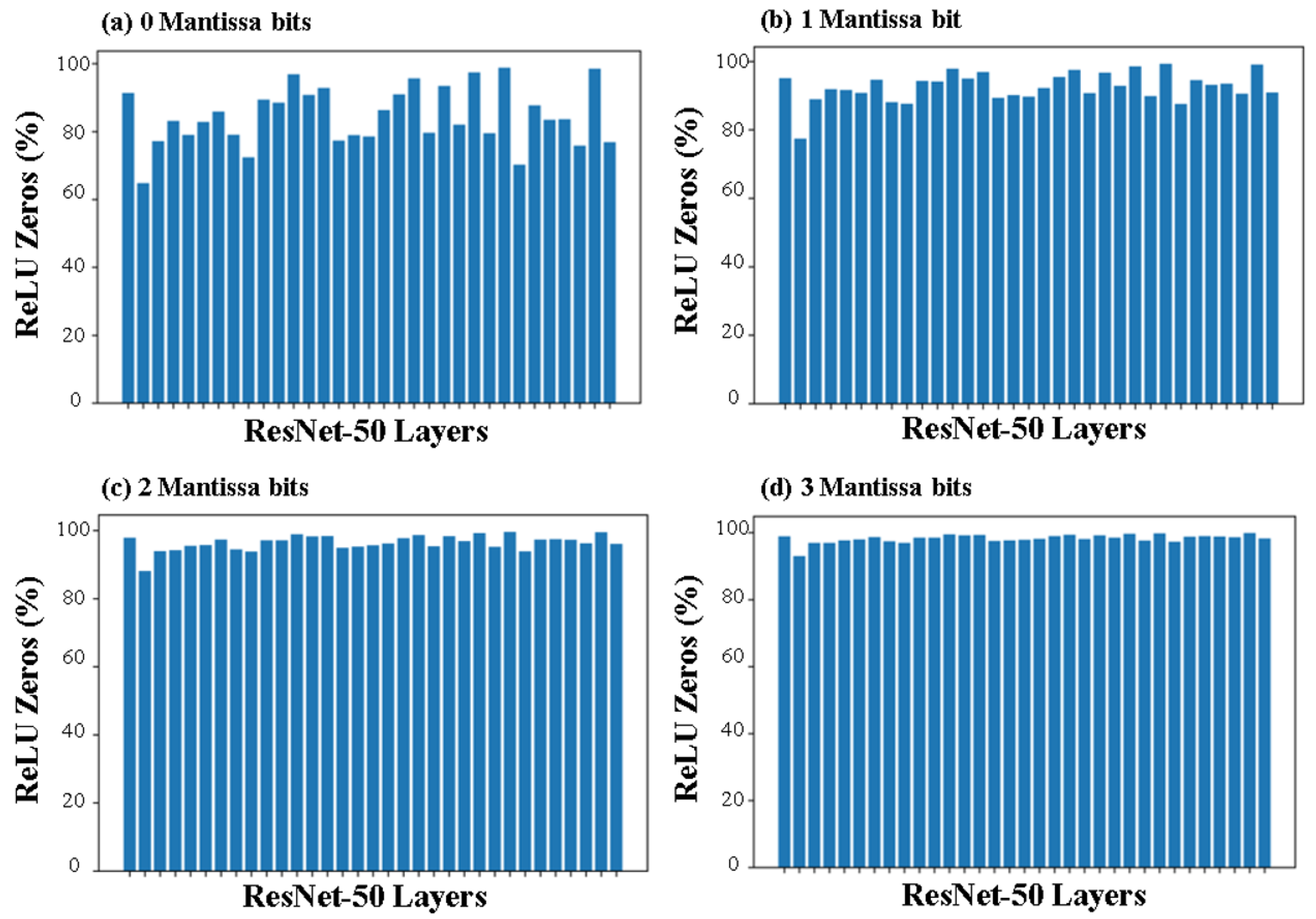
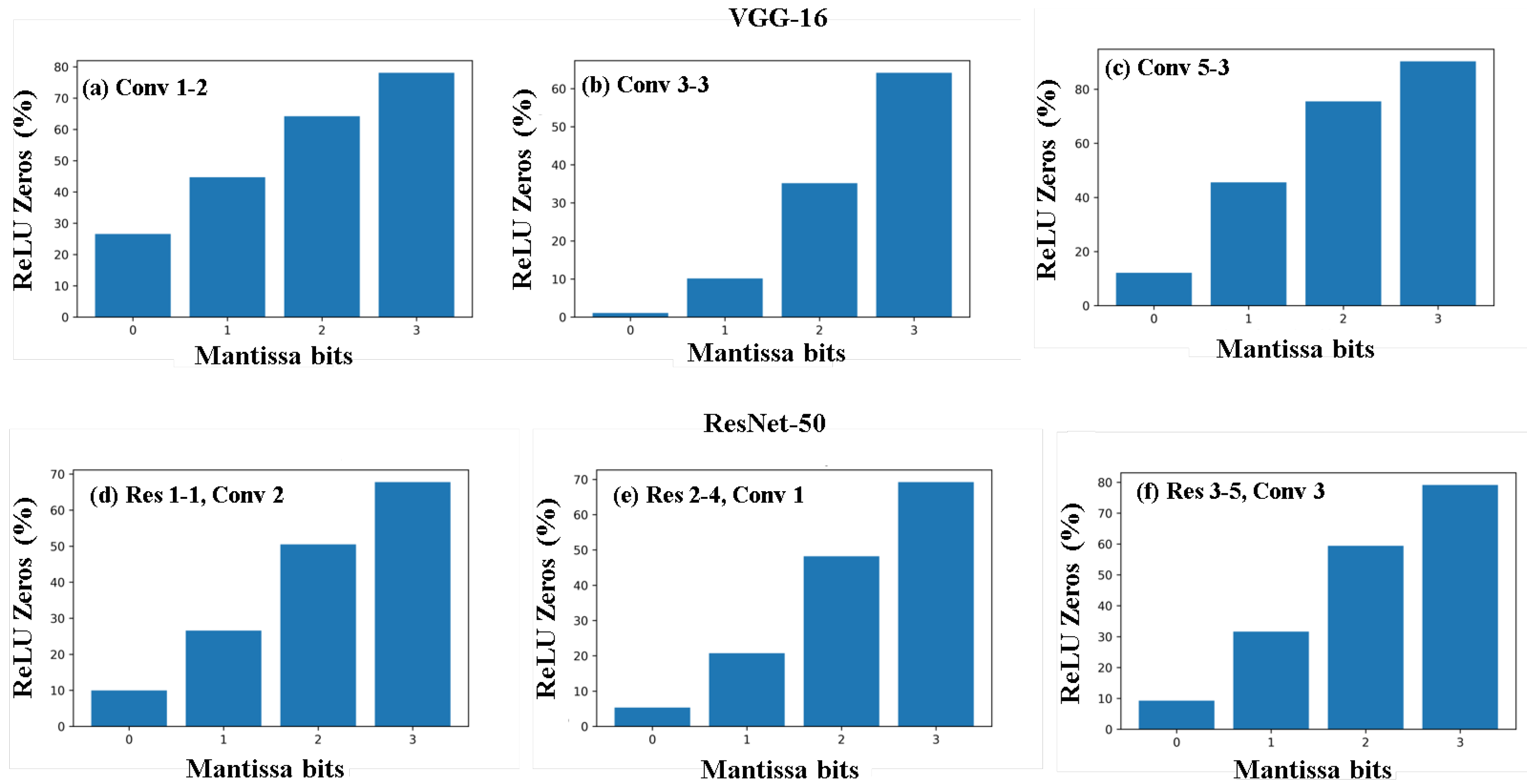
5. Results

In order to motivate the use of the hierarchical compute method to detect ReLU zeros early, we first identify the number of ReLU zeros that are present when a typical image is processed using the ResNet-50 and VGG-16 CNN models; findings are shown in Figure 8. It is evident from the figure that, in a majority of the layers, more than 50% of the ReLU outputs are zero, with many of the deeper layers having up to 90% ReLU zeros. Considering all the layers, we found that, on an average, 61.77% of the ReLU outputs were zeros in VGG-16, while 61.24% ReLU zeros were seen for ResNet-50. These results indicate that a large portion of compute is wasted on computing ReLU zeros, which can be avoided using the proposed method.
In addition to the percentage of ReLU zeros, it is also important to understand the distribution of values seen by the ReLU layer. The results from ResNet-50 layers are shown in Figure 9. A total of 10 bins were chosen—values below −8, −8 to −4, −4 to −2, −2 to −1, −1 to 0, 0 to 1, 1 to 2, 2 to 4, 4 to 8 and values above 8. We notice that, in all layers, about 50% of the values fall between −1 to 1, and more than 80% between −2 and 2. This implies that the majority of the values are close to zero. As a result, it is not practical to use a fixed threshold value along with reduced precision compute. A large negative threshold (say −2) can ensure that a value computed with reduced precision will have the correct sign. However, we can see from the distribution that only very few values (under 20%) can be detected with such a fixed threshold. If the threshold is pushed closer to zero, the chances of incorrectly detecting ReLU zeros increase. This study demonstrates the importance of the variable threshold derived using our model.
The proposed model was tested by evaluating the ReLU output values at different layers of both the VGG-16 and ResNet-50 CNN implementation. This was done by comparing the outputs from the convolution layer using (25) and (28). The total number of negative values that were detected using our model were noted and compared with the total number of output values to provide the percentage of negative values that are detected early. This was repeated for different layers, with different numbers of mantissa bits. Figure 10 shows the percentage of ReLU zeros detected by our model across different layers of ResNet-50 with different numbers of mantissa bits. It is evident that, as the number of mantissa bits considered increases, our model is able to detect the majority of ReLU zeros in all layers.
To get a closer look at the impact of increasing the number of mantissa bits, we plotted the percentage of ReLU zeros detected with 0, 1, 2, and 3 mantissa bits for randomly chosen layers in VGG-16 and ResNet-50. This is shown in Figure 11. As expected, the fraction of negative values detected increases as the number of mantissa bits used for computation is increased. Close to 80% of negative values can be detected early using just three mantissa bits, which can result in a significant increase in the efficiency of the network. Due to the nature of weights, range of values, and so on, we observe that the results across different layers vary. However, as seen in Figure 10, the amount of variation decreases as we use more mantissa bits. Additionally, we note similar effectiveness of our model for both VGG-16 and ResNet-50, which shows that the model does not depend on the type of CNN implementation—it works based on the fundamental characteristics of MAC operations and floating-point numbers, which makes it a generalized solution for any CNN layer with a ReLU activation function.
From the results presented, we see that about 60% of the outputs of the ReLU activation function are zero values in CNNs like VGG-16 and ResNet-50. If three mantissa bits are used for computation and our model is deployed, 80% of these ReLU zeros can be detected. Hence, we can expect about 50% of the all ReLU outputs to be estimated early. This way, almost half of the total computations can be carried out in low precision and the other half can be computed in full precision, while ensuring no loss in accuracy.

6. Discussion

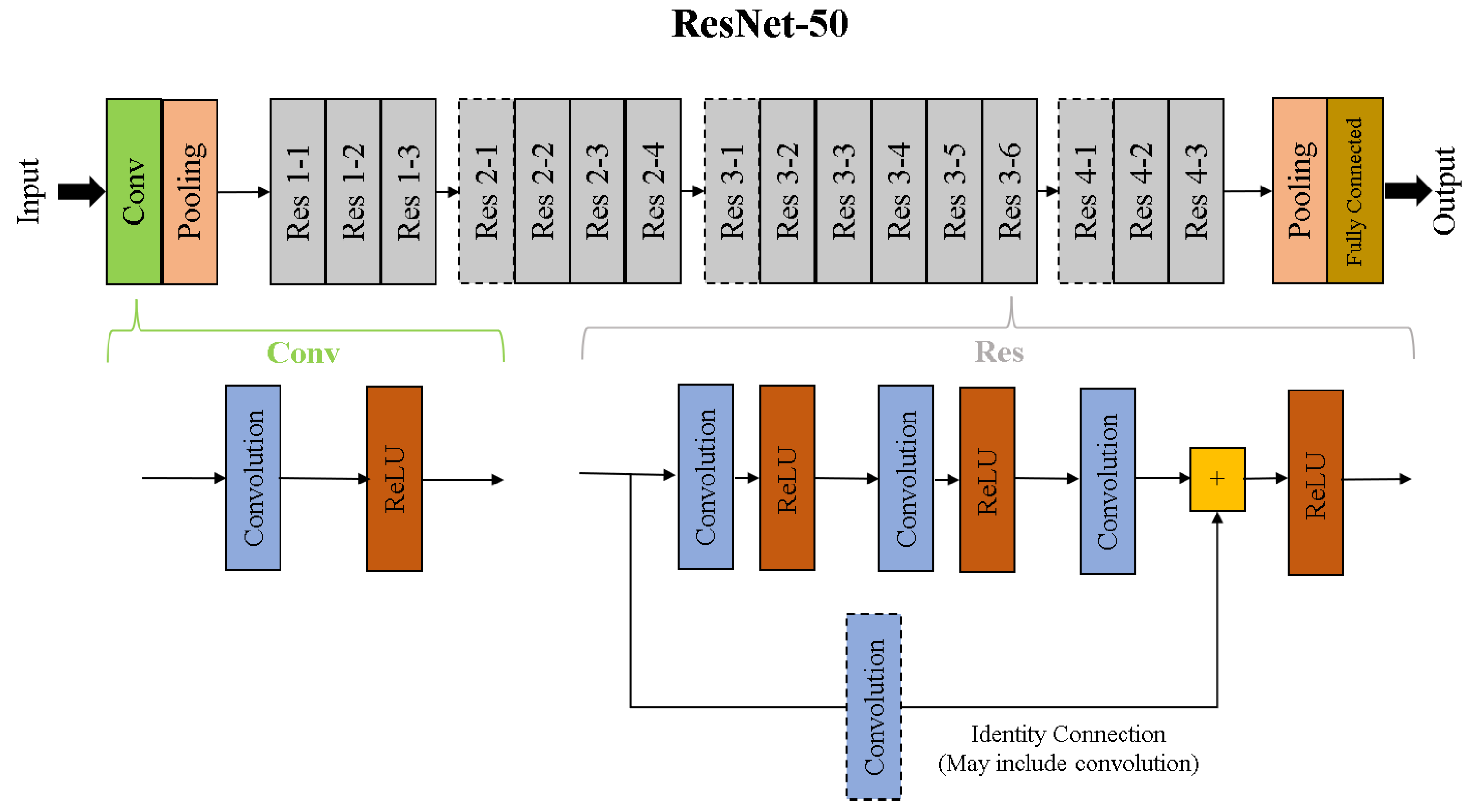
6.1. Generalization to Other DNNs

The results presented in this work utilize CNNs as the end application due to their ubiquitous nature and applicability to various fields. However, the model we have proposed is built on fundamental properties of floating-point numbers, MAC operations, and the ReLU activation function. Hence, the model can be extended to other applications too. When there are no negative values in the whole process, the algorithm will not predict any outcome and bypass all MAC output as valid output. However, these computations that are bypassed by algorithms as valid will be reused as a partial product for computing the actual output with the remaining mantissa bits. Since the compute used for prediction is re-purposed as a partial product and also for the cases which are slightly uncertain, the algorithm tends to predict them as positive value (no approximation) and bypass them out of the algorithm as valid outputs such that it will always go through the full precision compute. Hence, no accuracy drop is expected with the use of a proposed solution.
The proposed solution will be applicable across various networks with activation functions which displays a nonlinear behavior for either positive or negative numbers (not both) and the other one must be a zero or any constant value. To support activation functions like sigmoid, we might need to redevelop mathematical constraints to predict values between [−ve, +ve] range, while all other values outside this range can be set to a constant.

6.2. Implementation on GPU/Other Accelerators

This method is implementable on any compute engine that supports DNN workload. Since the proposed solution supports the reusing of partially computed elements that were used for early prediction, this will not impose a heavy tax on the existing hardware. On GPU and other accelerators, the proposed solution will need fine-tuning of data flow, data storage pattern and control logic, etc.

6.3. Extension to Training

The results presented in this work demonstrate the effectiveness of our model during the inference stage in a DNN. However, the process of training also involves the same set of steps, along with the additional step of adjusting the parameters. Hence, our model can be used in every layer with a ReLU activation layer. Since DNN training is a time-consuming and compute intensive process, this method can provide a significant improvement. It is also noteworthy to mention that, unlike inference, training must be done with high precision values. As a result, many of the approximate computing methods that have been studied cannot be extended to training. However, since our method ensures that there is no loss in accuracy, it can be applied to training as well.

7. Conclusions

In this work, we proposed a mathematical model that can detect zero outputs of the ReLU activation function using low-precision MAC operations. Our model takes into account the error resulting from the reduction of the number of bits in a floating-point representation, and identifies values that would be negative even when full-precision compute is performed. Our model can adapt based on the number of mantissa bits considered in the computation, ensuring its suitability for different number formats used in DNNs. We show that around 80% of ReLU zeros can be detected using just three mantissa bits, which corresponds to a total of 50% of all ReLU outputs in VGG16 and ResNet50 CNN implementations. As the model is developed with no assumption about the nature of the network or the application, we claim that the model can be extended to all DNNs that use the ReLU activation function. In addition, as the MAC operation and the activation layer in DNN training is identical to inference, this model can be adopted to make the compute-hungry training process more efficient. We also propose a system level model to implement this method and perform hardware acceleration of DNNs. The widespread use of DNNs with the ReLU activation function means that our model can be used as an error-free way to reduce computations in numerous applications.

Author Contributions

Conceptualization, B.S., K.P. and G.S.K.; writing—original draft preparation, B.S.; writing—review and editing, K.P. and G.S.K.; supervision, A.A. and S.S. All authors have read and agreed to the published version of the manuscript.

Funding

This research received no external funding.

Institutional Review Board Statement

Not applicable.

Informed Consent Statement

Not applicable.

Data Availability Statement

The dataset used for this study is publicly available and can be downloaded at https://www.image-net.org (accessed on 1 May 2021).

Conflicts of Interest

The authors declare no conflict of interest.

Abbreviations

The following abbreviations are used in this manuscript:
DNNDeep Neural Network
ReLURectified Linear Unit
VGGVisual Geometry Group
ResNetResidual Network
MACMultiply And Accumulate
GPUGraphics Processing Unit
CNNConvolutional Neural Network
IEEEInstitute of Electrical and Electronics Engineers
ILSVRCImageNet Large Scale Visual Recognition Challenge

References

  1. Liu, W.; Wang, Z.; Liu, X.; Zeng, N.; Liu, Y.; Alsaadi, F.E. A survey of deep neural network architectures and their applications. Neurocomputing 2017, 234, 11–26. [Google Scholar] [CrossRef]
  2. Zhang, L.; Zhang, Y. Big data analysis by infinite deep neural networks. Jisuanji Yanjiu Yu Fazhan/Comput. Res. Dev. 2016, 53, 68–79. [Google Scholar] [CrossRef]
  3. Strubell, E.; Ganesh, A.; McCallum, A. Energy and Policy Considerations for Deep Learning in NLP. In Proceedings of the ACL 2019—57th Annual Meeting of the Association for Computational Linguistics, Florence, Italy, 28 July–2 August 2019; pp. 3645–3650. [Google Scholar]
  4. Harlap, A.; Narayanan, D.; Phanishayee, A.; Seshadri, V.; Devanur, N.; Ganger, G.; Gibbons, P. PipeDream: Fast and Efficient Pipeline Parallel DNN Training. arXiv 2018, arXiv:1806.03377. [Google Scholar]
  5. Deng, C.; Liao, S.; Xie, Y.; Parhi, K.K.; Qian, X.; Yuan, B. PERMDNN: Efficient Compressed DNN Architecture with Permuted Diagonal Matrices. In Proceedings of the 2018 51st Annual IEEE/ACM International Symposium on Microarchitecture (MICRO), Fukuoka, Japan, 20–24 October 2018; pp. 189–202. [Google Scholar]
  6. Duggal, J.K.; El-Sharkawy, M. Shallow squeezenext: An efficient shallow DNN. In Proceedings of the 2019 IEEE International Conference on Vehicular Electronics and Safety (ICVES), Cairo, Egypt, 4–6 September 2019. [Google Scholar] [CrossRef]
  7. Wei, W.; Xu, L.; Jin, L.; Zhang, W.; Zhang, T. AI Matrix—Synthetic Benchmarks for DNN. arXiv 2018, arXiv:1812.00886. [Google Scholar]
  8. Hanif, M.A.; Javed, M.U.; Hafiz, R.; Rehman, S.; Shafique, M. Hardware–Software Approximations for Deep Neural Networks. In Approximate Circuits; Springer International Publishing: Cham, Switzerland, 2019; pp. 269–288. [Google Scholar] [CrossRef]
  9. Agrawal, A.; Choi, J.; Gopalakrishnan, K.; Gupta, S.; Nair, R.; Oh, J.; Prener, D.A.; Shukla, S.; Srinivasan, V.; Sura, Z. Approximate computing: Challenges and opportunities. In Proceedings of the 2016 IEEE International Conference on Rebooting Computing (ICRC), San Diego, CA, USA, 17–19 October 2016. [Google Scholar] [CrossRef]
  10. Liu, B.; Wang, Z.; Guo, S.; Yu, H.; Gong, Y.; Yang, J.; Shi, L. An energy-efficient voice activity detector using deep neural networks and approximate computing. Microelectron. J. 2019, 87, 12–21. [Google Scholar] [CrossRef]
  11. Zhu, H.; Akrout, M.; Zheng, B.; Pelegris, A.; Jayarajan, A.; Phanishayee, A.; Schroeder, B.; Pekhimenko, G. Benchmarking and Analyzing Deep Neural Network Training. In Proceedings of the 2018 IEEE International Symposium on Workload Characterization (IISWC), Raleigh, NC, USA, 30 September–2 October 2018; pp. 88–100. [Google Scholar] [CrossRef]
  12. Nwankpa, C.; Ijomah, W.; Gachagan, A.; Marshall, S. Activation Functions: Comparison of trends in Practice and Research for Deep Learning. arXiv 2018, arXiv:1811.03378. [Google Scholar]
  13. Wang, Y.; Li, Y.; Song, Y.; Rong, X. The Influence of the Activation Function in a Convolution Neural Network Model of Facial Expression Recognition. Appl. Sci. 2020, 10, 1897. [Google Scholar] [CrossRef] [Green Version]
  14. Alom, M.Z.; Taha, T.M.; Yakopcic, C.; Westberg, S.; Sidike, P.; Nasrin, M.S.; Van Esesn, B.C.; Awwal, A.A.S.; Asari, V.K. The history began from alexnet: A comprehensive survey on deep learning approaches. arXiv 2018, arXiv:1803.01164. [Google Scholar]
  15. Shi, S.; Chu, X. Speeding up convolutional neural networks by exploiting the sparsity of rectifier units. arXiv 2017, arXiv:1704.07724. [Google Scholar]
  16. Simonyan, K.; Zisserman, A. Very deep convolutional networks for large-scale image recognition. In Proceedings of the International Conference on Learning Representations (ICLR), San Diego, CA, USA, 7–9 May 2015. [Google Scholar]
  17. He, K.; Zhang, X.; Ren, S.; Sun, J. Deep residual learning for image recognition. In Proceedings of the IEEE Conference on Computer Vision and Pattern Recognition, Las Vegas, NV, USA, 27–30 June 2016; pp. 770–778. [Google Scholar] [CrossRef] [Green Version]
  18. Albericio, J.; Delmás, A.; Judd, P.; Sharify, S.; O’Leary, G.; Genov, R.; Moshovos, A. Bit-pragmatic deep neural network computing. In Proceedings of the 50th Annual IEEE/ACM International Symposium on Microarchitecture, Cambridge, MA, USA, 14–18 October 2017; pp. 382–394. [Google Scholar]
  19. Albericio, J.; Judd, P.; Hetherington, T.; Aamodt, T.; Jerger, N.E.; Moshovos, A. Cnvlutin: Ineffectual-neuron-free deep neural network computing. ACM SIGARCH Comput. Archit. News 2016, 44, 1–13. [Google Scholar] [CrossRef]
  20. Chen, T.; Du, Z.; Sun, N.; Wang, J.; Wu, C.; Chen, Y.; Temam, O. Diannao: A small-footprint high-throughput accelerator for ubiquitous machine-learning. ACM SIGARCH Comput. Archit. News 2014, 42, 269–284. [Google Scholar] [CrossRef]
  21. Judd, P.; Albericio, J.; Hetherington, T.; Aamodt, T.M.; Moshovos, A. Stripes: Bit-serial deep neural network computing. In Proceedings of the 2016 49th Annual IEEE/ACM International Symposium on Microarchitecture (MICRO), Taipei, Taiwan, 15–19 October 2016; pp. 1–12. [Google Scholar]
  22. Chen, Y.H.; Krishna, T.; Emer, J.S.; Sze, V. Eyeriss: An energy-efficient reconfigurable accelerator for deep convolutional neural networks. IEEE J. Solid-State Circuits 2016, 52, 127–138. [Google Scholar] [CrossRef] [Green Version]
  23. Gao, M.; Pu, J.; Yang, X.; Horowitz, M.; Kozyrakis, C. Tetris: Scalable and efficient neural network acceleration with 3d memory. In Proceedings of the Twenty-Second International Conference on Architectural Support for Programming Languages and Operating Systems, Xi’an, China, 8–12 April 2017; pp. 751–764. [Google Scholar]
  24. Hua, W.; Zhou, Y.; De Sa, C.; Zhang, Z.; Suh, G.E. Boosting the performance of cnn accelerators with dynamic fine-grained channel gating. In Proceedings of the 52nd Annual IEEE/ACM International Symposium on Microarchitecture, Columbus, OH, USA, 12–16 October 2019; pp. 139–150. [Google Scholar]
  25. Chen, C.Y.; Choi, J.; Gopalakrishnan, K.; Srinivasan, V.; Venkataramani, S. Exploiting approximate computing for deep learning acceleration. In Proceedings of the 2018 Design, Automation & Test in Europe Conference & Exhibition (DATE), Dresden, Germany, 19–23 March 2018; pp. 821–826. [Google Scholar]
  26. Gupta, S.; Agrawal, A.; Gopalakrishnan, K.; Narayanan, P. Deep Learning with Limited Numerical Precision. In Proceedings of the 32nd International Conference on Machine Learning (ICML 2015), Lille, France, 6–11 July 2015; Volume 3, pp. 1737–1746. [Google Scholar]
  27. Judd, P.; Albericio, J.; Hetherington, T.; Aamodt, T.; Jerger, N.E.; Urtasun, R.; Moshovos, A. Reduced-Precision Strategies for Bounded Memory in Deep Neural Nets. arXiv 2015, arXiv:1511.05236. [Google Scholar]
  28. Shafique, M.; Hafiz, R.; Javed, M.U.; Abbas, S.; Sekanina, L.; Vasicek, Z.; Mrazek, V. Adaptive and Energy-Efficient Architectures for Machine Learning: Challenges, Opportunities, and Research Roadmap. In Proceedings of the 2017 IEEE Computer Society Annual Symposium on VLSI (ISVLSI), Bochum, Germany, 3–5 July 2017; pp. 627–632. [Google Scholar] [CrossRef]
  29. Sarwar, S.S.; Srinivasan, G.; Han, B.; Wijesinghe, P.; Jaiswal, A.; Panda, P.; Raghunathan, A.; Roy, K. Energy efficient neural computing: A study of cross-layer approximations. IEEE J. Emerg. Sel. Top. Circuits Syst. 2018, 8, 796–809. [Google Scholar] [CrossRef]
  30. Venkatesh, G.; Nurvitadhi, E.; Marr, D. Accelerating Deep Convolutional Networks using low-precision and sparsity. In Proceedings of the 2017 IEEE International Conference on Acoustics, Speech and Signal Processing (ICASSP), New Orleans, LA, USA, 5–9 March 2017; pp. 2861–2865. [Google Scholar]
  31. Liu, B.; Guo, S.; Qin, H.; Gong, Y.; Yang, J.; Ge, W.; Yang, J. An energy-efficient reconfigurable hybrid DNN architecture for speech recognition with approximate computing. In Proceedings of the 2018 IEEE 23rd International Conference on Digital Signal Processing (DSP), Shanghai, China, 19–21 November 2018; pp. 1–5. [Google Scholar]
  32. Ardakani, A.; Leduc-Primeau, F.; Onizawa, N.; Hanyu, T.; Gross, W.J. VLSI implementation of deep neural network using integral stochastic computing. IEEE Trans. Very Large Scale Integr. (VLSI) Syst. 2017, 25, 2688–2699. [Google Scholar] [CrossRef] [Green Version]
  33. Niu, W.; Ma, X.; Lin, S.; Wang, S.; Qian, X.; Lin, X.; Wang, Y.; Ren, B. Patdnn: Achieving real-time dnn execution on mobile devices with pattern-based weight pruning. In Proceedings of the Twenty-Fifth International Conference on Architectural Support for Programming Languages and Operating Systems, Lausanne, Switzerland, 16–20 March 2020; pp. 907–922. [Google Scholar]
  34. Sarker, M.M.K.; Rashwan, H.; Akram, F.; Singh, V.K.; Banu, S.F.; Chowdhury, F.; Choudhury, K.; Chambon, S.; Radeva, P.; Puig, D.; et al. SLSNet: Skin lesion segmentation using a lightweight generative adversarial network. Expert Syst. Appl. 2021, 183, 115433. [Google Scholar] [CrossRef]
  35. Han, S.; Mao, H.; Dally, W.J. Deep compression: Compressing deep neural networks with pruning, trained quantization and huffman coding. arXiv 2015, arXiv:1510.00149. [Google Scholar]
  36. Courbariaux, M.; Bengio, Y.; David, J.P. Training deep neural networks with low precision multiplications. arXiv 2014, arXiv:1412.7024. [Google Scholar]
  37. Louizos, C.; Reisser, M.; Blankevoort, T.; Gavves, E.; Welling, M. Relaxed quantization for discretized neural networks. arXiv 2018, arXiv:1810.01875. [Google Scholar]
  38. Chernikova, A.; Oprea, A.; Nita-Rotaru, C.; Kim, B. Are self-driving cars secure? Evasion attacks against deep neural networks for steering angle prediction. In Proceedings of the 2019 IEEE Security and Privacy Workshops (SPW), San Francisco, CA, USA, 19–23 May 2019; pp. 132–137. [Google Scholar]
  39. Pustokhina, I.V.; Pustokhin, D.A.; Gupta, D.; Khanna, A.; Shankar, K.; Nguyen, G.N. An effective training scheme for deep neural network in edge computing enabled Internet of medical things (IoMT) systems. IEEE Access 2020, 8, 107112–107123. [Google Scholar] [CrossRef]
  40. Sarker, M.M.K.; Makhlouf, Y.; Craig, S.G.; Humphries, M.P.; Loughrey, M.; James, J.A.; Salto-Tellez, M.; O’Reilly, P.; Maxwell, P. A Means of Assessing Deep Learning-Based Detection of ICOS Protein Expression in Colon Cancer. Cancers 2021, 13, 3825. [Google Scholar] [CrossRef]
  41. Li, Z.; Zhang, Y.; Wang, J.; Lai, J. A survey of FPGA design for AI era. J. Semicond. 2020, 41, 021402. [Google Scholar] [CrossRef]
  42. Dean, J. Machine learning for systems and systems for machine learning. In Proceedings of the 2017 Conference on Neural Information Processing Systems, Long Beach, CA, USA, 4–9 December 2017. [Google Scholar]
  43. Shomron, G.; Banner, R.; Shkolnik, M.; Weiser, U. Thanks for nothing: Predicting zero-valued activations with lightweight convolutional neural networks. In Proceedings of the European Conference on Computer Vision, Glasgow, UK, 23–28 August 2020; pp. 234–250. [Google Scholar]
  44. Akhlaghi, V.; Yazdanbakhsh, A.; Samadi, K.; Gupta, R.K.; Esmaeilzadeh, H. Snapea: Predictive early activation for reducing computation in deep convolutional neural networks. In Proceedings of the 2018 ACM/IEEE 45th Annual International Symposium on Computer Architecture (ISCA), Los Angeles, CA, USA, 1–6 June 2018; pp. 662–673. [Google Scholar]
  45. Asadikouhanjani, M.; Ko, S.B. A novel architecture for early detection of negative output features in deep neural network accelerators. IEEE Trans. Circuits Syst. II Express Briefs 2020, 67, 3332–3336. [Google Scholar] [CrossRef]
  46. Kim, C.; Shin, D.; Kim, B.; Park, J. Mosaic-CNN: A combined two-step zero prediction approach to trade off accuracy and computation energy in convolutional neural networks. IEEE J. Emerg. Sel. Top. Circuits Syst. 2018, 8, 770–781. [Google Scholar] [CrossRef]
  47. Chang, J.; Choi, Y.; Lee, T.; Cho, J. Reducing MAC operation in convolutional neural network with sign prediction. In Proceedings of the 2018 International Conference on Information and Communication Technology Convergence (ICTC), Jeju Island, Korea, 17–19 October 2018; pp. 177–182. [Google Scholar]
  48. Lin, Y.; Sakr, C.; Kim, Y.; Shanbhag, N. PredictiveNet: An energy-efficient convolutional neural network via zero prediction. In Proceedings of the 2017 IEEE International Symposium on Circuits and Systems (ISCAS), Baltimore, MD, USA, 28–31 May 2017; pp. 1–4. [Google Scholar]
  49. Song, M.; Zhao, J.; Hu, Y.; Zhang, J.; Li, T. Prediction based execution on deep neural networks. In Proceedings of the 2018 ACM/IEEE 45th Annual International Symposium on Computer Architecture (ISCA), Los Angeles, CA, USA, 1–6 June 2018; pp. 752–763. [Google Scholar]
  50. Sze, V.; Chen, Y.H.; Yang, T.J.; Emer, J.S. Efficient Processing of Deep Neural Networks: A Tutorial and Survey. Proc. IEEE 2017, 105, 2295–2329. [Google Scholar] [CrossRef] [Green Version]
  51. Agarap, A.F. Deep learning using rectified linear units (relu). arXiv 2018, arXiv:1803.08375. [Google Scholar]
  52. Kepner, J.; Gadepally, V.; Jananthan, H.; Milechin, L.; Samsi, S. Sparse deep neural network exact solutions. In Proceedings of the 2018 IEEE High Performance extreme Computing Conference (HPEC), Waltham, MA USA, 25–27 September 2018; pp. 1–8. [Google Scholar]
  53. Talathi, S.S.; Vartak, A. Improving performance of recurrent neural network with relu nonlinearity. arXiv 2015, arXiv:1511.03771. [Google Scholar]
  54. Kahan, W. IEEE standard 754 for binary floating-point arithmetic. Lect. Notes Status IEEE 1996, 754, 11. [Google Scholar]
  55. Russakovsky, O.; Deng, J.; Su, H.; Krause, J.; Satheesh, S.; Ma, S.; Huang, Z.; Karpathy, A.; Khosla, A.; Bernstein, M.; et al. ImageNet Large Scale Visual Recognition Challenge. Int. J. Comput. Vis. 2014, 115, 211–252. [Google Scholar] [CrossRef] [Green Version]
  56. Chollet, F. and others.; Keras. 2015. Available online: https://keras.io (accessed on 1 May 2021).
  57. Abadi, M.; Agarwal, A.; Barham, P.; Brevdo, E.; Chen, Z.; Citro, C.; Corrado, G.S.; Davis, A.; Dean, J.; Devin, M.; et al. TensorFlow: Large-Scale Machine Learning on Heterogeneous Systems. Software. 2015. Available online: tensorflow.org (accessed on 1 May 2021).
Figure 1. Example of the convolution operation. In this example, the stride is assumed to be 1. A 5 × 5 output is produced from the 7 × 7 input when a 3 × 3 weight matrix is considered.
Mathematics 09 03130 g001
Figure 2. Graphical representation of the ReLU function. If x is the input and y is the output, then y = 0 for x < 0, and y = x for x ≥ 0.
Mathematics 09 03130 g002
Figure 3. IEEE 754 floating point representation [54]. The total bits are divided into sign, exponent, and mantissa. The single precision format has 1 sign, 8 exponents, and 23 mantissa bits, while the double precision has 1 sign, 11 exponents, and 52 mantissa bits.
Mathematics 09 03130 g003
Figure 4. VGG-16 CNN architecture. There are 16 computation layers (13 convolution 3 × 3 kernel and three fully connected layers without dropout). Pooling layers are present in the intermediate stages to reduce the layer size as the network gets deeper. Regularization, normalization, and other layers may be present but have not been shown in this figure for simplicity.
Mathematics 09 03130 g004
Figure 5. ResNet-50 Architecture. There are 50 computations layers (excluding convolution layers in the identity path) between the input and output. This includes 49 convolution layers and the fully-connected layer at the end. Res 2–1 (conv with 1 × 1, 64; 3 × 3, 64; 1 × 1, 256), Res 3–1 (1 × 1, 128; 3 × 3, 128; 1 × 1, 512) and Res 4–1 (1 × 1, 256; 3 × 3, 256; 1 × 1, 1024) are shown with a dotted boundary to indicate that they include a convolution layer along their identity path (also shown with a dotted boundary in the elaboration below without dropout). Regularization, normalization, and other layers may be present but have not been shown in this figure for simplicity.
Mathematics 09 03130 g005
Figure 6. Flow chart depicting the steps to perform hierarchical compute (three steps) and detect ReLU zeros with reduced precision. The first step is to perform MAC using exponent and predict ReLU output; if undetermined, compute most significant 8-bits of mantissa and check ReLU again if still not conclusive perform compute using remaining mantissa bits (every next step uses previously computed values). Here, the red arrows depict writing to the memory, and blue arrows indicate read from memory. Black arrows indicate that the computation has been completed for the given input.
Mathematics 09 03130 g006
Figure 7. Intuition behind estimating ReLU zeros based on reduced precision compute. In the hierarchical compute method, the value of “n” (number of MSB mantissa bits) is increased at each step, resulting in a decrease in the region of interest, until only positive values are remaining.
Mathematics 09 03130 g007
Figure 8. Percentage of ReLU zeros present in (a) VGG16; (b) ResNet50 when a typical image is processed through the models. Only a few layers of ResNet-50 are shown for clarity—a similar trend is observed in all the layers.
Mathematics 09 03130 g008
Figure 9. Distribution of ReLU inputs in different layers of ResNet-50. Here, Val is the input to the ReLU function. A total of 10 bins have been considered, and the range in each bin in mentioned in the figure. The different layers shown in the figure are: (a) first convolution layer from the input image (b) first convolution layer in the Res 1-1 block; (c) first convolution layer in the Res 2-1 block; (d) first convolution layer in the Res 3-1 block.
Mathematics 09 03130 g009
Figure 10. Percentage of ReLU values detected using our model across different ResNet-50 layers. The first 33 convolution layers are shown in the figure. The number of MSB mantissa bits used were (a) 0; (b) 1; (c) 2; and (d) 3.
Mathematics 09 03130 g010
Figure 11. Percentage of ReLU zeros identified by our model when different mantissa bits were considered. The figure shows the results in (a) Conv 1-2; (b) Conv 3-3; and (c) Conv 5-3 layers of VGG-16, and (d) second convolution layer of Res 1-1 block; (e) first convolution layer of Res 2-4 block; and (f) third convolution layer of Res 3-5 block. Similar results were observed in other layers of both ResNet-50 and VGG-16.
Mathematics 09 03130 g011
Publisher’s Note: MDPI stays neutral with regard to jurisdictional claims in published maps and institutional affiliations.

