Prediction of Hydraulic Jumps on a Triangular Bed Roughness Using Numerical Modeling and Soft Computing Methods

Abstract

This study investigates the characteristics of free and submerged hydraulic jumps on the triangular bed roughness in various T/I ratios (i.e., height and distance of roughness) using CFD modeling techniques. The accuracy of numerical modeling outcomes was checked and compared using artificial intelligence methods, namely Support Vector Machines (SVM), Gene Expression Programming (GEP), and Random Forest (RF). The results of the FLOW-3D^® model and experimental data showed that the overall mean value of relative error is 4.1%, which confirms the numerical model’s ability to predict the characteristics of the free and submerged jumps. The SVM model with a minimum of Root Mean Square Error (RMSE) and a maximum of correlation coefficient (R²), compared with GEP and RF models in the training and testing phases for predicting the sequent depth ratio (y₂/y₁), submerged depth ratio (y₃/y₁), tailwater depth ratio (y₄/y₁), length ratio of jumps ($L_j/y_2^{*}$) and energy dissipation (ΔE/E₁), was recognized as the best model. Moreover, the best result for predicting the length ratio of free jumps $(L_{jf/}{y}_2^{*}$) in the optimal gamma is γ = 10 and the length ratio of submerged jumps $(L_{js/}{y}_2^{*}$) is γ = 0.60. Based on sensitivity analysis, the Froude number has the greatest effect on predicting the (y₃/y₁) compared with submergence factors (SF) and T/I. By omitting this parameter, the prediction accuracy is significantly reduced. Finally, the relationships with good correlation coefficients for the mentioned parameters in free and submerged jumps were presented based on numerical results.

1. Introduction

The hydraulic jump is a natural phenomenon in an open channel, sometimes regarded as an effective method of energy dissipation near structures such as gates, chutes, and spillways [1]. The hydraulic jump is specified by the expansion of large-scale turbulence, surface waves and spray, energy dissipation, and air entrainment [2]. If the tailwater depth equals the subcritical sequent depth, it is called a free hydraulic jump. Furthermore, if the tailwater depth is greater than the subcritical sequent depth, the jump is submerged (submerged hydraulic jump). A hydraulic jump has been widely studied, but only a few investigations have regarded the effect of bed roughness on the characteristics of hydraulic jumps. Enormous research studies dealing with the free and submerged hydraulic jumps such as McCorquodale and Khalifa [3], Smith [4], Graber et al. [5], Vallé and Pasternack [6], Dey and Sarkar [7], Tokyay et al. [8], and Samadi-Boroujeni et al. [9] were carried out. Ead and Rajaratnam [10] experimentally studied hydraulic jumps on corrugated beds.

The results showed that the length of jumps was about half of those on smooth beds. Carollo et al. [11] investigated the hydraulic jump properties on a bed roughened by gravel particles. The results indicate that the roughness reduces the sequent depth and the length of the jump. Pagliara et al. [12] studied the hydraulic jump on homogeneous and non-homogeneous rough beds. The results satisfactorily matched with the experimental data and presented new equations to estimate the length of jump and sequent depth. Abbaspour et al. [13] investigated the impact of a corrugated bed on hydraulic jumps. The results stated that the jump length and tailwater depth on corrugated beds are smaller than the smooth bed. Chanson [14] observed the flow resistance effects in decreasing the sequence depth ratio for a given Froude number. The results indicated that the Bélanger equation is not appropriate. In addition, the cross-sectional properties of irregular channels have an important influence on the flow characteristics. Ahmed et al. [15] investigated the effect of bed roughness on the submerged jump. Conclusions show that the length of a jump and tailwater depth on a bed roughness are smaller than on a smooth bed. Palermo and Pagliara [16] produced two general equations for evaluating relative energy dissipation across various hydraulic and geometrical conditions. Pourabdollah et al. [17] studied free and submerged jumps in different stilling basins. They showed that the sequent depth, the submerged depth, and the length of the jump decreased compared to the classical jump. Moreover, the average energy dissipation of the submerged jump on the bed roughness was more than those of the classical jump. Habibzadeh et al. [18] investigated characteristics of hydraulic jumps with and without blocks. The mean longitudinal velocity, turbulence intensity, Turbulent Kinetic Energy (TKE), and shear stress and water surface fluctuations were studied and compared for various flow regimes.

In addition to laboratory research, numerical works have been done on hydraulic jumps. Gharangik and Chaudhry [19] solved the 1D Boussinesq equations to simulate a hydraulic jump in a rectangular channel. The results showed that the equation terms have little influence in determining the location of the hydraulic jump. Ma et al. [20] investigated the turbulence characteristics of 2D submerged hydraulic jumps using the k–ε turbulence model. The results are compared with available experimental data and are acceptable. Mousavi et al. [21] investigated predictive modeling of the free hydraulic jumps pressure through advanced statistical methods. It was verified that maximum and minimum pressure fluctuation are located near the spillway toe and downstream of hydraulic jumps, respectively. Abbaspour et al. [22] numerically studied hydraulic jump on a corrugated bed using the standard k-ε and RNG turbulent models. Their results stated that the k-ε model was suitable for predicting the jump characteristics. Chern and Syamsuri [23] applied the Smoothed Particle Hydrodynamics (SPH) model to evaluate characteristics of the hydraulic jump in different corrugated beds and classified jump. Bayon et al. [24] investigated the performance of Open-FOAM and FLOW-3D^® software in the numerical investigation of the hydraulic jump. Nikmehr and Aminpour [25] investigated the characteristics of a hydraulic jump over bed roughness with trapezoidal blocks using the CFD model. The results state that increasing the distance and the height of the roughness will decrease the velocity near the bed and increase the shear stress. Ghaderi et al. [26] numerically investigated the characteristics of the hydraulic jumps over various roughness shapes using the FLOW-3D^® model. The results were compared with previous studies. Relationships with good correlation coefficients for the mentioned parameters in free and submerged jumps were presented based on numerical results. Ghaderi et al. [27] studied the effects of triangular microroughness on the characteristics of the submerged jump with the help of the FLOW-3D^® model. To validate the present model, comparisons between numerical simulations and experimental results were performed for the smooth bed and triangular microroughness [27].

Recent advancements in data-driven models, i.e., Gene Expression Programming (GEP) and Artificial Neural Networks (ANN), and their application in hydraulics engineering have challenged the conventional techniques of the analysis. Several researchers have shown that soft computing techniques are more feasible and accurate than conventional techniques.

Karbasi and Azamathulla [28] studied free hydraulic jump characteristics in the bed roughness using Support Vector Regression (SVR), GEP, and ANN methods. The results showed the GEP model has better accuracy than other methods. Roushangar and Ghasempour [29] studied hydraulic jump characteristics in sudden expanding channels using GEP. The results showed the GEP model has better accuracy and was compared with existing empirical equations. Roushangar and Ghasempour [30] predicted the hydraulic jump energy dissipation using an SVM with channel geometry and roughness boundary conditions. The sensitivity analysis results stated that the Froude number had the most important impact on the modeling. Roushangar and Homayounfar [31] investigated the characteristics of hydraulic jumps on horizontal and sloping beds using the SVM method. Results verify that the upstream Froude number is the most critical and influential parameter for predicting the sequent depth in free and submerged jumps. At the same time, Naseri and Othman [32] predicted the length of jump on the smooth beds using ANN. Nasrabadi et al. [33] studied submerged hydraulic jump characteristics using machine learning methods. According to the evaluation, the Developed Group Method of Data Handling (DGMDH) model is more accurate than the Group Method Data Handling (GMDH) model and other previous research predicting the submergence depth and jump length relative energy dissipation.

Many studies have been carried out on hydraulic jumps over smooth beds. Nevertheless, few studies have investigated the effect of bed roughness and corresponding characteristics of free and submerged jumps numerically and predicted the outcomes from the numerical models using novel soft computing techniques. Hence, the main objectives of this study are the investigation of the effects of bed roughness parameters considering various roughness arrangements on characteristics of the free and submerged jumps, such as sequent depth and submerged depth, the length of jumps, and energy dissipation in triangular bed roughness through different hydraulic conditions with the CFD technique (CFD is a numerical methodology commonly used in engineering [34]), and verification of the prediction of this numerical model with the help of soft computing methods (SVM, GEP, and RF).

2. Materials and Methods

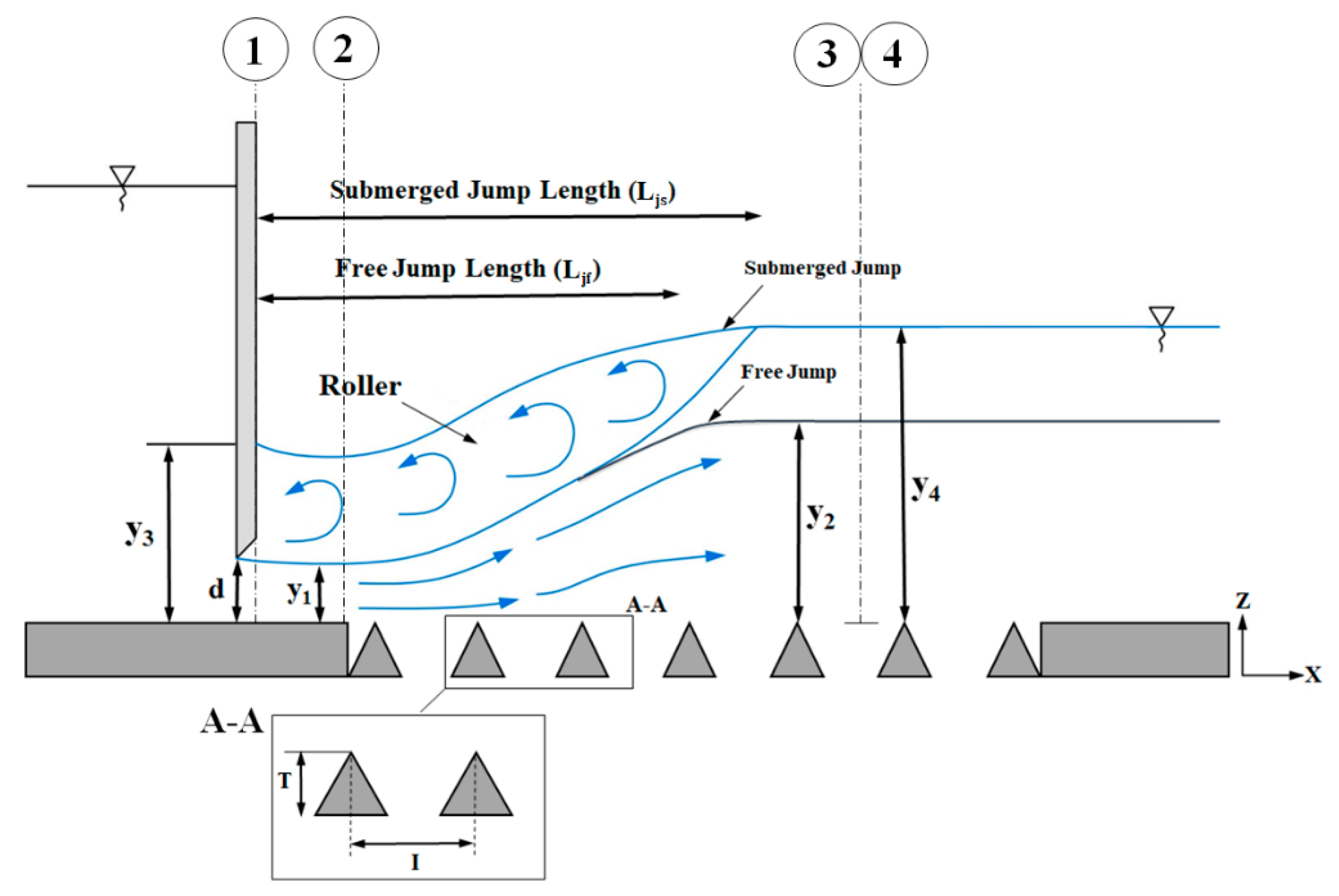
2.1. Dimensional Analysis

The hydraulic jumps characteristics on bed roughness are dependent on fluid properties, bed dimensions, and hydraulic state of flow. Therefore, subcritical of the free jump depth (y₂) and submerged of the submerged jump depth (y₃) will be a function of the following parameters:

$$y_2=f_1(y_1,u_1,g,\mu ,\rho ,T,I)$$

(1)

$$y_3=f_2(y_1,y_2,y_4,u_1,g,\mu ,\rho ,T,I)$$

(2)

Using the dimensional analysis, the following relationships are obtained:

$$\frac{y_2}{y_1}=f_3(F{r}_1=\frac{u_1}{\sqrt[]{g{y}_1}},{\mathrm{Re}}_1=\frac{y_1{}_{}{u}_1}{\nu },\frac{T}{y_1},\frac{T}{I})$$

(3)

$$\frac{y_3}{y_1}=f_4(F{r}_1=\frac{u_1}{\sqrt[]{g{y}_1}},{\mathrm{Re}}_1=\frac{y_1{}_{}{u}_1}{\nu },SF=\frac{y_4-y_2}{y_2},\frac{T}{y_1},\frac{T}{I})$$

(4)

where y₁ and y₄ are referred to as supercritical of the free jump depth and tailwater of the submerged jump depth; u₁ is inlet velocity; and g, ρ, μ, SF, and υ are the gravity acceleration, mass density of water, water dynamic viscosity, submergence factors, and water kinematic viscosity, respectively. T and I are height and distance of roughness, and Fr₁ and Re₁ are Froude and Reynolds numbers, respectively. The values of the Reynolds number (Re₁) were in the range of 39,884–59,825. For large values of the Reynolds number, viscous effects can be neglected [35,36,37]. Based on the Ead and Rajaratnam [10] and Abbaspour et al. [22] studies, T/y₁ does not significantly affect the hydraulic jumps’ depth ratio y₂/y₁ and y₃/y₁. Then, relationships (3) and (4) become:

$$\frac{y_2}{y_1}=f_5(F{r}_1,\frac{T}{I})$$

(5)

$$\frac{y_3}{y_1}=f_6(F{r}_1,SF=\frac{y_4-y_2}{y_2},\frac{T}{I})$$

(6)

Using the Buckingham Π theorem, for the length of jump on the free and submerged jumps (L_jf/y₂ and L_js/y₂), the following relationships are obtained:

$$\frac{L_{jf}}{y_2^{}}=f_7(F{r}_1,\frac{T}{I})$$

(7)

$$\frac{L_{js}}{y_2^{}}=f_8(F{r}_1,SF=\frac{y_4-y_2}{y_2},\frac{T}{I})$$

(8)

Figure 1 shows a schematic view of free and submerged jumps on the triangular bed roughness, along with critical hydraulic parameters of the present study. In this figure, d is gate opening.

2.2. The FLOW-3D^® Model

Numerical simulations were carried out using FLOW-3D, a well-known and established computational fluid dynamics software. This software uses the finite volume method in a Cartesian, staggered grid to solve the RANS equations (Reynolds Average Navier−Stokes) that describe continuity and momentum and are expressed as:

$$\frac{\partial }{\partial x}(u{A}_x)+\frac{\partial }{\partial y}(v{A}_y)+\frac{\partial }{\partial z}(w{A}_z)=0$$

(9)

$$\frac{\partial U_i}{\partial t}+\frac{1}{V_F}\left(u_j{A}_j\frac{\partial u_i}{\partial x_j}\right)=-\frac{1}{\rho }\frac{\partial P}{\partial x_i}+G_i+f_i$$

(10)

where u, v, and w represent the components of velocity in the x, y, and z-direction; V_F is the volume fraction of fluid in each cell; A_x, A_y, and A_z are the fractional areas open to flow in the subscript’s direction; ρ is the fluid density; P is the hydrostatic pressure; G_i is the gravitational acceleration in subscript direction; and f_i is the Reynolds stress. In FLOW-3D, free surfaces are modeled with the Volume of Fluid (VOF) technique and developed by Hirt and Nichols [37]. The VOF transport equation is expressed by the following equation:

$$\frac{\partial F}{\partial t}+\frac{1}{V_F}\left[\frac{\partial (F{A}_x{u}_1)}{\partial x}+\frac{\partial (F{A}_y{u}_2)}{\partial y}+\frac{\partial (F{A}_z{u}_3)}{\partial z}\right]=0$$

(11)

Here, F denotes the fraction function. In particular, as already stated, if a cell is empty, then F = 0, and if a cell is full, then F = 1 [38]. The free surface is determined at a position related to intermediate amounts of F (i.e., the user may usually determine F = 0.5, or another intermediate amount).

2.2.1. Turbulence Model

In this study, the RNG k-ε turbulence model is used to simulate the turbulence in the water flow. The RNG k-ε model improves the standard k-ε model (Equations (12) and (13)), reflecting small-scale effects by large-scale motion and modified viscosity terms, and can handle the flow with a large degree of curvature well [39]. This model showed satisfactory outcomes in previous studies on hydraulic engineering studies in complex geometry and flow fields [26,27,40,41,42,43,44,45,46].

$$\frac{\partial (\rho k)}{\partial t}+\frac{\partial (\rho k{u}_i)}{\partial x_i}=\frac{\partial }{\partial x_j}({\alpha }_k{\mu }_{eff}\frac{\partial k}{\partial x_j})+G_k+\rho \epsilon$$

(12)

$$\frac{\partial (\rho \epsilon )}{\partial t}+\frac{\partial (\rho \epsilon u_i)}{\partial x_i}=\frac{\partial }{\partial x_j}({\alpha }_{\epsilon }{\mu }_{eff}\frac{\partial \epsilon }{\partial x_j})+\frac{C_{1\epsilon }^{*}\epsilon }{k}{G}_k-C_{2\epsilon }\rho \frac{{\epsilon }^2}{k}$$

(13)

Here, k is called turbulent kinetic energy (TKE); ε is the turbulence dissipation rate; G_k is the generation of turbulent kinetic energy caused by the average velocity gradient; G_b is the generation of turbulent kinetic energy caused by buoyancy. S_k and S_ε are source terms. ${\alpha }_k$, ${\alpha }_{\epsilon }$ and μ_eff, $C_{2\epsilon }$, $C_{1\epsilon }^{*}$ are model constants is effective viscosity.

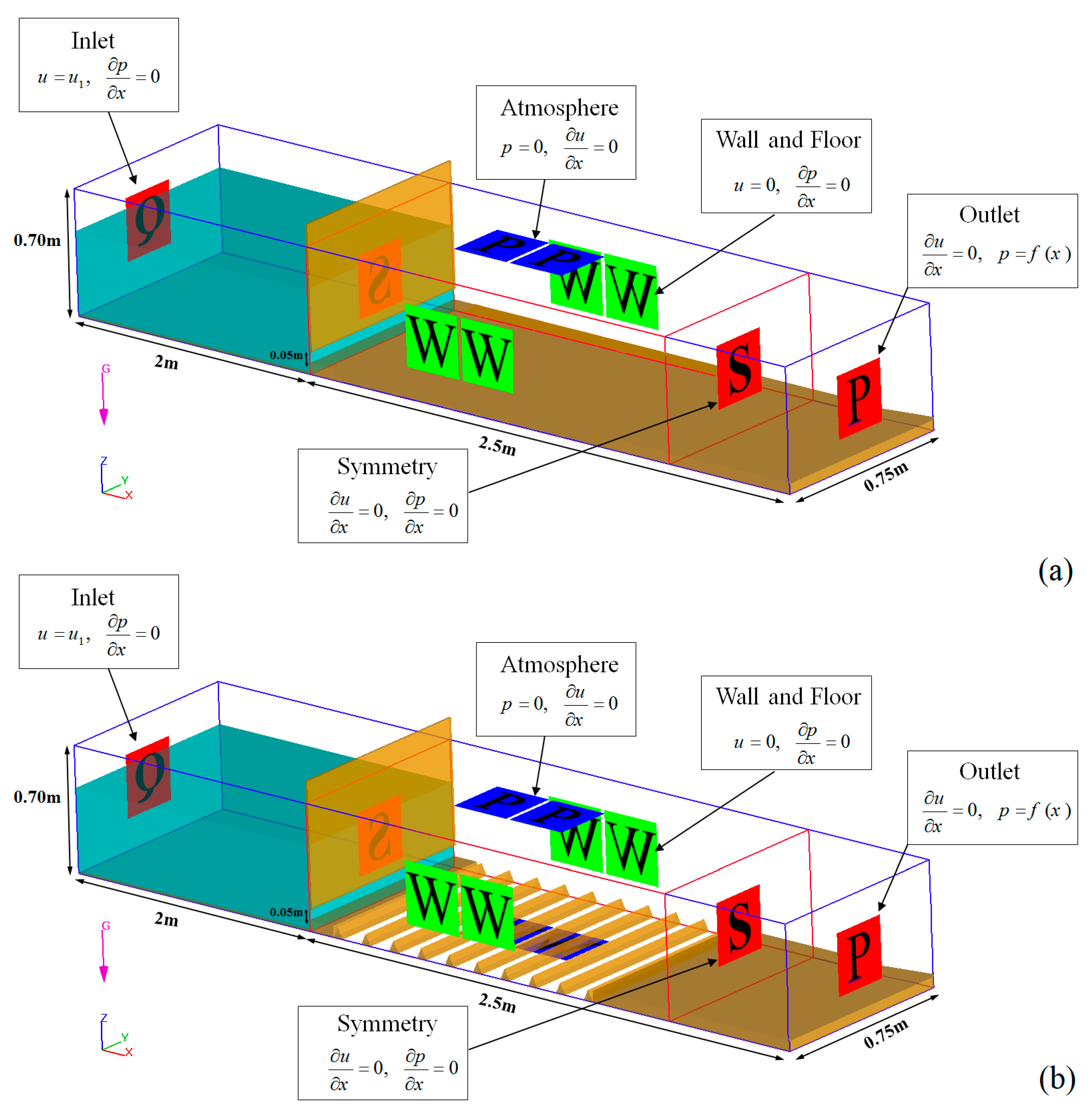
2.2.2. Boundary Conditions

Corresponding to the physical conditions of the problem, four different boundary conditions were considered. Hence, the inlet and the exit boundary of the first mesh block needed to be set in the flow direction. The inlet boundary condition was set as discharge flow rate (Q) with flow depth at the channel’s beginning. The boundary condition at the downstream end of the domain was described by a pressure boundary condition (P) corresponding to the tailwater depth in the flume. No-slip conditions were applied at the wall boundaries and the bottom, and they were treated as non-penetrative boundaries. Wall roughness has been neglected due to the slight roughness of the material of the experimental facility, which was used for validation. An atmospheric boundary condition is set to the upper boundary of the channel. This allows the flow to enter and leave the domain as null von Neumann conditions are imposed to all variables except for pressure, which is set to zero (i.e., atmospheric pressure). The symmetry (S) is used at the inner boundaries as well. Figure 2 shows the computational domain of the present study and the boundary conditions governing the simulation.

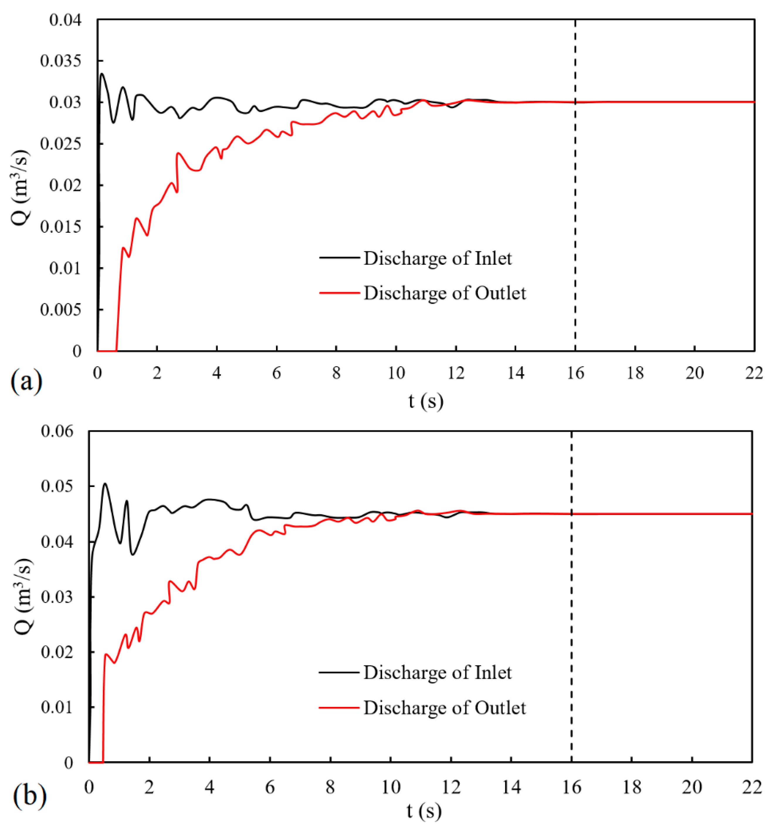
2.2.3. Checking Stability and Convergence Criterion

To obtain the correct numerical or experimental model data values, it is necessary to reach a stable state. A stability criterion similar to the Courant number is used to calculate the allowed time-step size. The Courant Number tells how fast the fluid passes through a cell. If the Courant Number is greater than 1, the velocity of the fluid is so high that it passes through a cell in less than one time step. This leads to numerical instabilities: the stability criteria leading to time steps between 0.001 s and 0.0016 s. The evolution in time was used as a relaxation to the final steady state. During the simulations, the solutions’ steady-state convergence was checked by monitoring the flow discharge variations at the inlet and outlet boundaries. Figure 3 shows that t = 16 s is appropriate to achieve a near steady-state condition for Q = 0.03 m³/s and Q = 0.045 m³/s. The computational time for the simulations was between 14–18 h using a personal computer with eight cores of a CPU (Intel Core i7-7700K @ 4.20 GHz and 16 GB RAM).

2.2.4. Numerical Domain

The research provided by Ahmed et al. [15] compares the numerical model and laboratory test results. Although the length of the experimental flume was 24.5 m, the present numerical study is set equal to 4.5 m to improve the performance in terms of computational effort and reduction in the number of overall cells [26] (for more details, see Ahmed et al. [15]).

Table 1. The parameters of the numerical models.

Bed Type	Q (m3/s)	I (cm)	T (cm)	d (cm)	y1 (cm)	y4 (cm)	Fr1	SF
Smooth	0.03, 0.045	-	-	5	1.62–3.83	9.64–32.10	1.7–9.3	0.26–0.50
Triangular roughness	0.03, 0.045	4–8–12–16–20	4	5	1.62–3.84	6.82–30.08	1.7–9.3	0.21–0.44

shows the parameters of the numerical models.

The geometry of the models is built represented through an STL (stereolithography) file. The numerical mesh is constructed to adopt two mesh blocks, a containing mesh block for the entire spatial domain and a nested block with refined cells for the area of interest. The hydraulic jump occurs (Figure 4). The best practice is to have fixed points aligning the mesh boxes and for the aspect ratios to be no greater than 2.

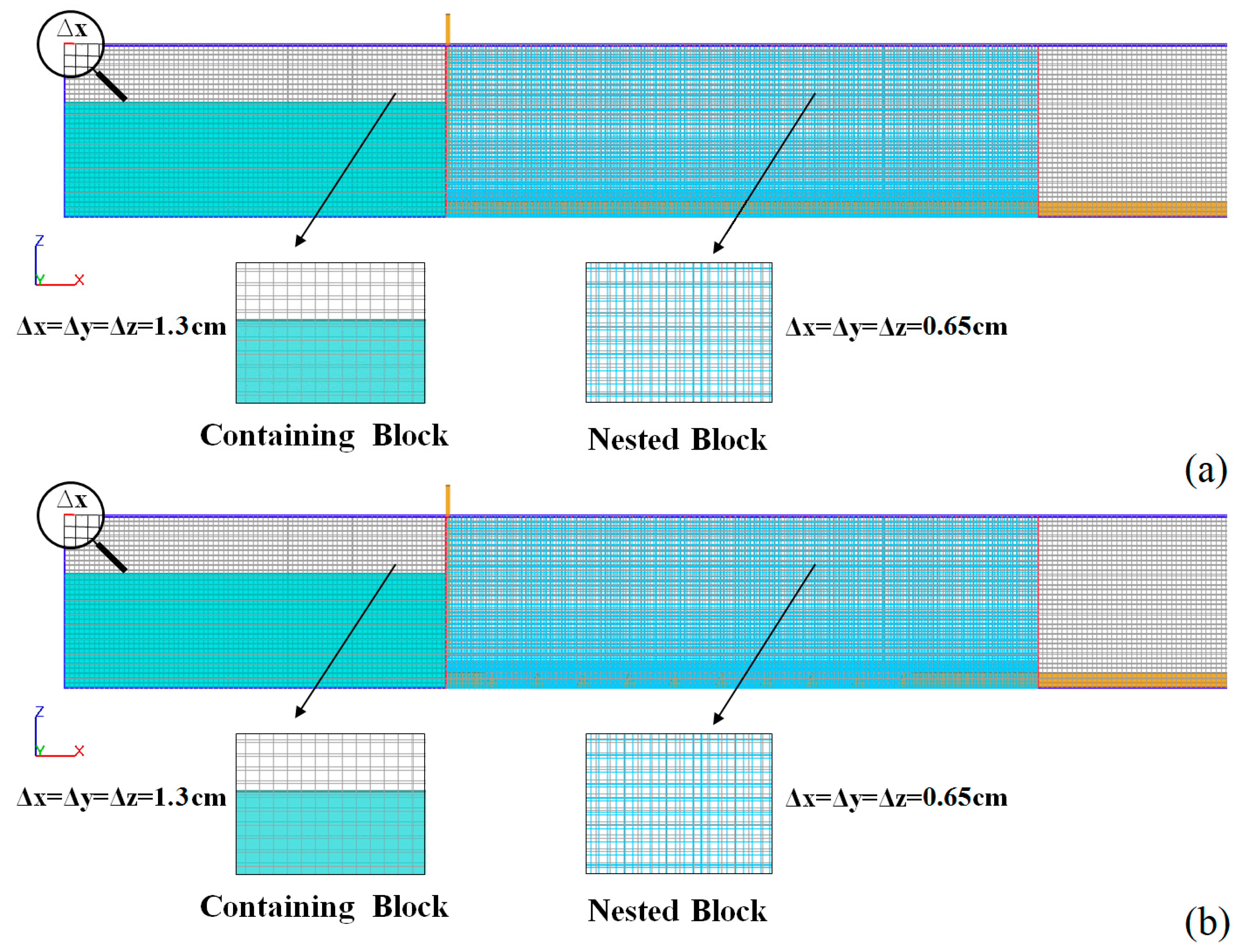
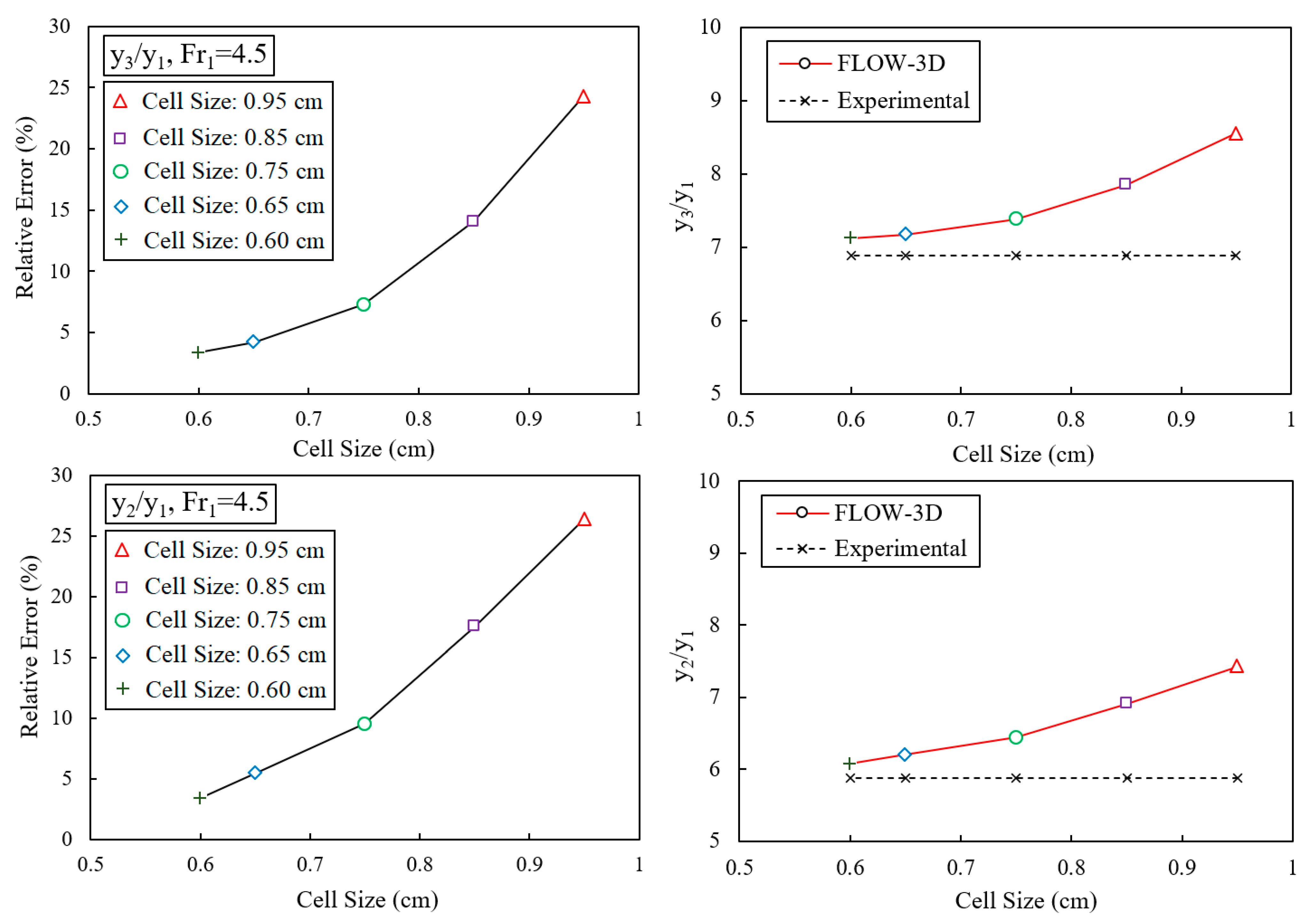
2.2.5. Mesh Size Sensitivity Analysis

According to the sensitivity mesh results and by comparing y₃/y₁ and y₂/y₁ ratios at Fr₁ = 4.5 for a submerged and free hydraulic jump, numerical solutions for five different mesh sizes at distances close to the computational grid were used.

Table 2. Mesh size sensitivity analysis for simulation.

Test No.	Coarser Cells Size (cm)	Finer Cells Size (cm)	Total Cells	(y3/y1)Num	(y3/y1)Exp	(y2/y1)Num	(y2/y1)Exp	MAPE 1-y3/y1 (%)	MAPE-y2/y1 (%)
T1	2.00	0.95	910,358	8.55	6.88	7.43	5.88	26.36	24.27
T2	1.70	0.85	1,285,482	7.85	6.88	6.91	5.88	17.51	14.09
T3	1.50	0.75	1,871,649	7.38	6.88	6.44	5.88	9.52	7.26
T4	1.30	0.65	2,908,596	7.17	6.88	6.20	5.88	5.44	4.21
T5	1.15	0.60	3,812,035	7.10	6.88	6.08	5.88	3.41	3.34

¹ Mean Absolute Percentage Error = $100\times \frac{1}{\mathrm{n}}{\displaystyle \sum _1^{\mathrm{n}}}\left|\frac{{\mathrm{X}}_{\mathrm{Exp}}-{\mathrm{X}}_{\mathrm{Num}}}{{\mathrm{X}}_{\mathrm{Exp}}}\right|$. X_Exp: the experimental value of X; X_Num: the numerical value of X; and n: the total amount of data.

provides a summary list of the results for three different mesh sizes. Figure 5 shows that the simulated y₃/y₁ and y₂/y₁ ratios exhibit better agreement with the measured y₃/y₁ and y₂/y₁ for the finer cell size of 0.60 cm. In addition, the variation of mean relative errors can be neglected by decreasing the cell size from 0.65 cm to 0.60 cm. As a result, the selected mesh consists of a containing block with 1.3 cm cells and a nested block with 0.65 cm cells. In the present research, the same mesh was utilized for all models to reduce the effect of computational mesh on simulation results. A distance of the first cell from the walls was selected to prevent computations in the viscous sub-layer.

2.3. Artificial Intelligence Methods

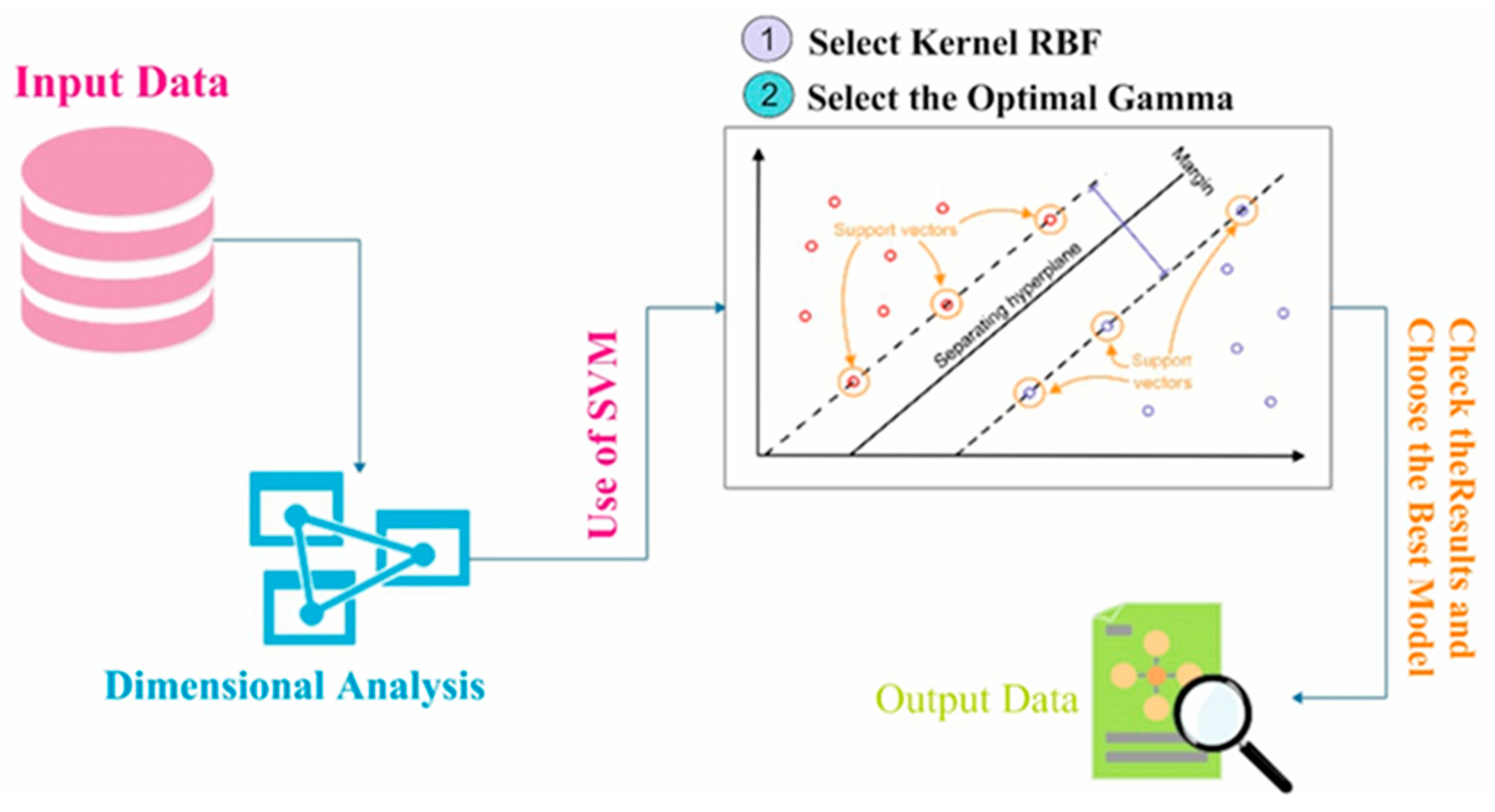
2.3.1. Support Vector Machine (SVM)

SVM algorithm is a data mining algorithm that uses the regression method to solve classification and prediction problems. Like artificial neural networks, problem-solving steps are divided into two phases of training and testing (i.e., validation). First, the system is trained by a part of data, then the problem’s solution is evaluated with test data. The SVM is based on linear data classification and tries to select a line with a high margin of confidence in the linear division of data. The training data closer to the separator page is called the support vector. The maximum distance between the two categories is known as the optimal separator page [47]. Based on the limited information of the samples, the SVM algorithm seeks the best option among the models with different complexities and the ability to train these models [48]. The SVM algorithm consists of four different kernels, which are presented in

Table 3. Types of kernel functions [50].

Function	Expression
Linear Kernel	$K\left(x_i,x_j\right)=\left(x_i,x_j\right)$
Polynomial Kernel	$K\left(x_i,x_j\right)={\left((x_i,x_j)\hspace{0.17em}+\hspace{0.17em}1\right)}^d$
Radial Basis Kernel	$K\left(x_i,x_j\right)=exp\left(-\frac{{\Vert x_i\hspace{0.17em}-\hspace{0.17em}{x}_j\Vert }^2}{2{\sigma }^2}\right)$
Sigmoid Kernel	$K\left(x_i,x_j\right)\hspace{0.17em}=\hspace{0.17em}tanh\left(-a(x_i,x_j)\hspace{0.17em}+\hspace{0.17em}c\right)$

. The most widely used kernel functions in support vector machine problems are Gaussian (RBF) and ring kernel (ERBF) functions [49]. These functions are used when information on the data type and their nature is not available in problem-solving [50]. In the present study, the RBF function has been used to predict the parameters.

Here, X_i and X_j are two vectors in directions i and j, and a, c, and d are Kernel parameters. According to Figure 6, first, the input data is entered into the statistical software. Based on dimensional analysis, the dependent and independent parameters are defined in the software environment by selecting the function (RBF) and entering the main feature of the SVM model of this function (i.e., γ by trial-and-error method). Selecting the appropriate values of γ makes the results accurate and close to reality.

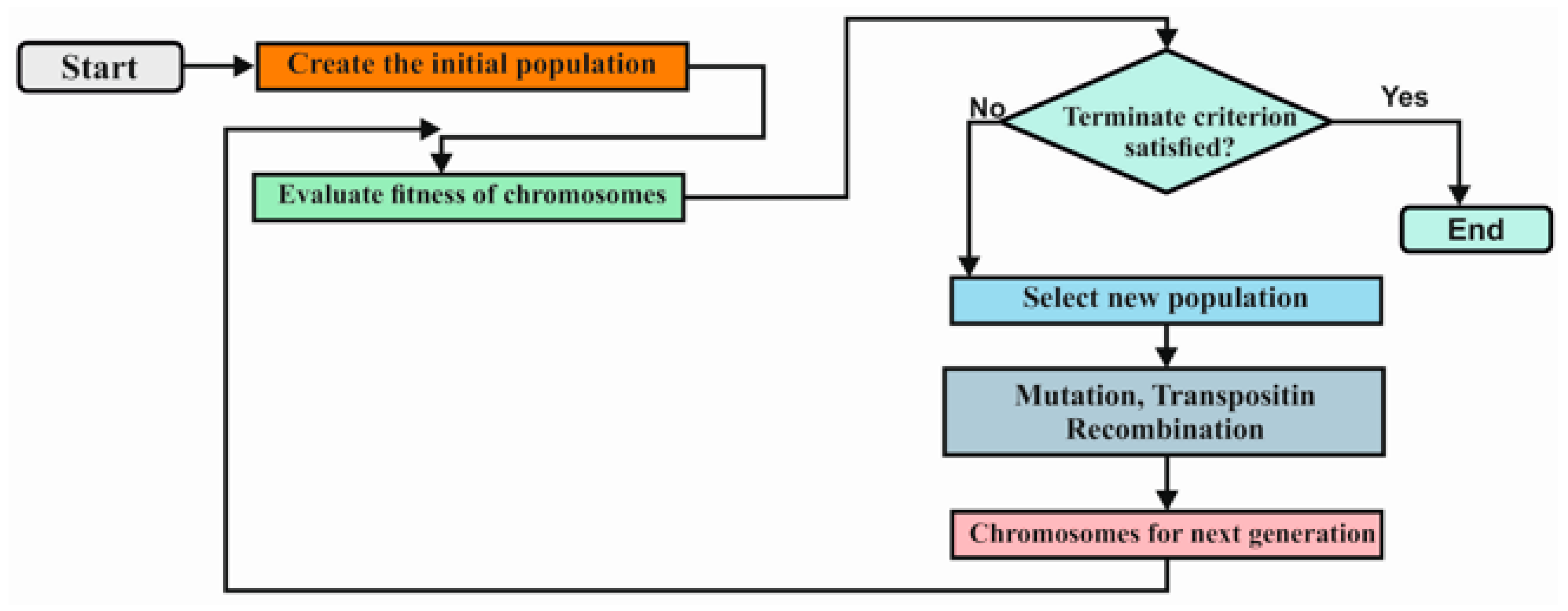
2.3.2. Gene Expression Programming (GEP)

The GEP method is a combined and developed Genetic Algorithm (GA) and Genetic Programming (GP) developed by Ferreira [51]. This method combines linear and simple chromosomes with constant length, similar to genetic algorithms, and branch structures of different sizes and shapes, similar to decomposition trees in genetic programming. The first step in the GEP is to form the initial population through solutions. Then, the chromosomes are shown as a tree (ETs). The fitness function determines the degree of compatibility of each member of the population of chromosomes. Next, the number of genes and chromosomes must be determined to run the GEP model. One of the strengths of the GEP is that the criterion for genetic diversity is very simple, so genetic operators operate at chromosomal levels. Another strength of this method is the unique nature of its multi-genes, which provides the basis for evaluating complex simulations [52]. The GEP algorithm consists of five steps: determining the fitness function, selecting the set of terminals and the set of functions to create the chromosomes, selecting the structure of the chromosomes, selecting the link function, and selecting the genetic operators and their rates [50,53]. In the present study, the GeneXproTools program was used to predict the parameters. The main steps of the GEP method are shown schematically in Figure 7.

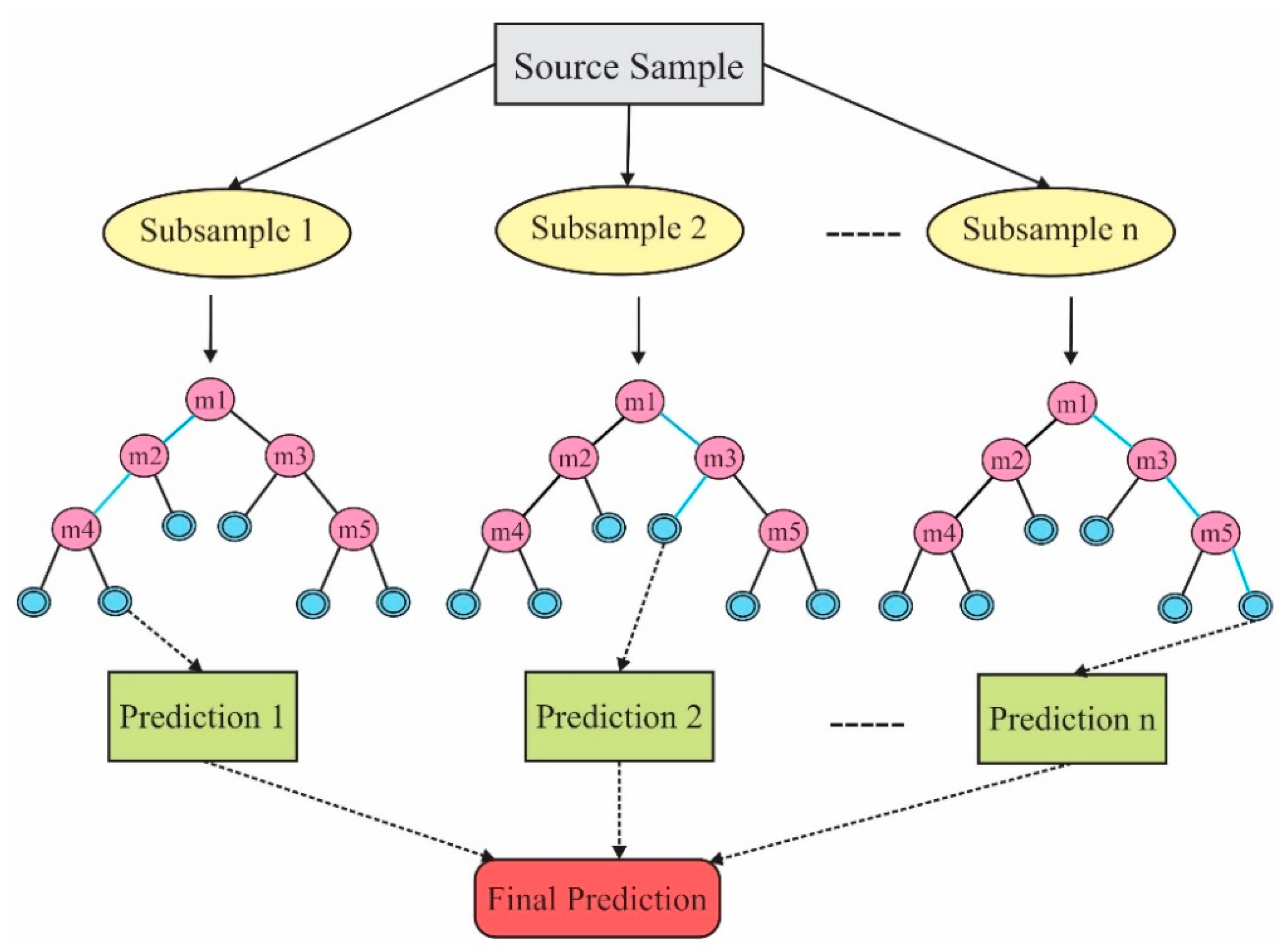
2.3.3. Random Forest (RF)

RF algorithm is currently one of the learning algorithms. This is a cumulative learning algorithm for regression-based problems and grouping based on decision tree development [54]. An RF is a collection of unpruned trees in which each tree is generated by a recursive segmentation algorithm [51]. In other words, an RF is a combination of several decision trees in which several self-organizing samples of data participate. The self-organizing method is the sampling method with placement. None of the selected data are deleted from the input samples to generate the following subset. Therefore, some data may be used more than once in educational branches. Others that have little effect on modeling should never be used. For the selective self-organizing sample, a classification tree is grown using the recursive segmentation algorithm. The analysis operation is based on a random sample of the number of predictor variables in each node. The recursive decomposition algorithm continues until the tree reaches its maximum size without pruning it [54]. The performance of the RF algorithm is shown in Figure 8.

2.4. Evaluation Criteria

In the present study, the evaluation criteria of correlation coefficient (R²), Root Mean Square Error (RMSE), Normalized Root Mean Square of Error (NRMSE), and Mean Absolute Percentage Error (MAPE) were used to compare the results of prediction models of hydraulic parameters of hydraulic jumps (Equations (14)–(17)).

$$R^2={\left(\frac{n\sum X_{Num}{X}_{Pre}-\left(\sum X_{Num}\right)\left(\sum X_{Pre}\right)}{\sqrt{n(\sum X_{Num}^2)-(\sum X_{Num}{)}^2}\sqrt{n(\sum X_{Pre}^2)-(\sum X_{Pre}{)}^2}}\right)}^2$$

(14)

$$RMSE=\sqrt{\frac{1}{n}{{\displaystyle \sum _1^n\left(X_{Num}-X_{Pre}\right)}}^2}$$

(15)

$$NRMSE(\%)=100\times \frac{\sqrt{\frac{1}{n}{{\displaystyle \sum _1^n\left(X_{Num}-X_{Pre}\right)}}^2}}{{\displaystyle \sum _1^n{X}_{Num}}}$$

(16)

$$MAPE(\%)=100\times \frac{1}{n}{\displaystyle \sum _1^n\left|\frac{X_{Num}-X_{Pre}}{X_{Num}}\right|}$$

(17)

Here, the X_Pre and the X_Num are the predicted and the numerical values. It should be noted that the best model is the model in which RMSE is zero and R² is one, and also NRMSE and MAPE values are less than 10%.

3. Results

In the present study, the output results of the FLOW-3D^® model were investigated using SVM, GEP, and RF methods. For this purpose, a total of 620 output data of numerical model were used to predict the parameters (y₂/y₁), (y₃/y₁), (y₄/y₁), ($L_j$/$y_2^{*}$), and (ΔE/E₁) with artificial intelligence methods. To achieve accurate prediction and better results, the training process was repeated several times. Finally, a pattern of 25% data for testing and 75% data for training was used for all methods.

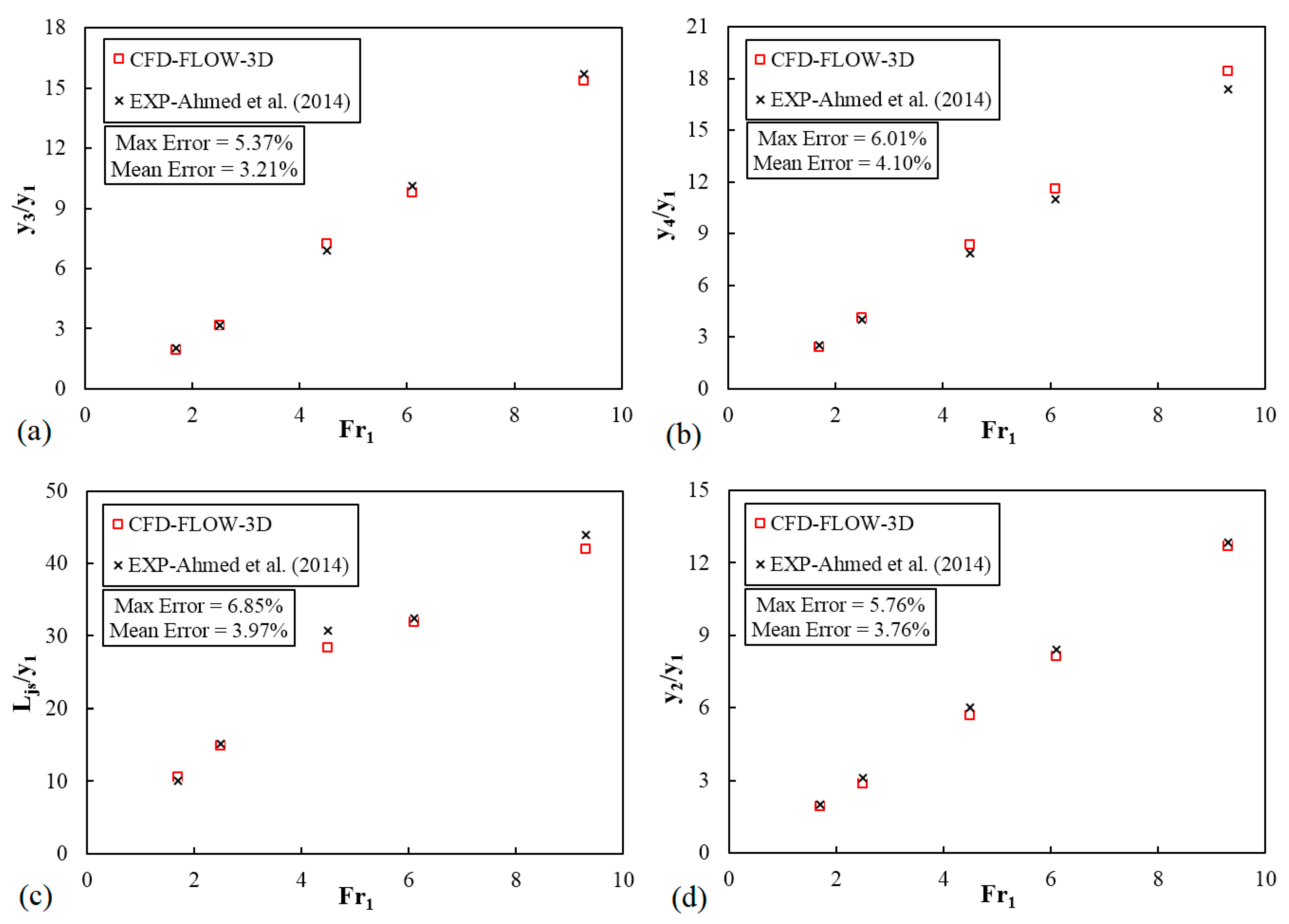
3.1. Validity of the FLOW-3D^® Model Results

Although the CFD technique has been on the rise for more than half a century, computers have only allowed us to solve more complex 3D geometries in the recent decade. Because of that, it is very important to validate CFD results [55]. Hence, a comparison between numerical and experimental results on basic parameters including submerged ratio (y₃/y₁), tailwater ratio (y₄/y₁), and relative jump length (L_js/y₁) of a submerged hydraulic jump and the sequent depth ratio (y₂/y₁) of a free hydraulic jump on a smooth bed have been used to validate the numerical model and are plotted in Figure 9.

Moreover, the essential flow variables are summarized in

Table 4. Basic flow variables for the numerical and physical models after Ahmed et al. [15].

Models	Bed	Q (m3/s)	d (cm)	y1 (cm)	u1 (m/s)	Fr1
Numerical and physical	Smooth	0.045	5	1.62–3.83	1.04–3.70	1.7–9.3

.

From the graphs, a substantial agreement can be observed between numerical and experimental results by Ahmed et al. [15] as a function of Fr₁. The overall mean value of relative error is 4.1%, which confirms the ability of the numerical model to predict the specifications of free and submerged jumps. In general, the CFD model is in excellent agreement with the experimental data [56].

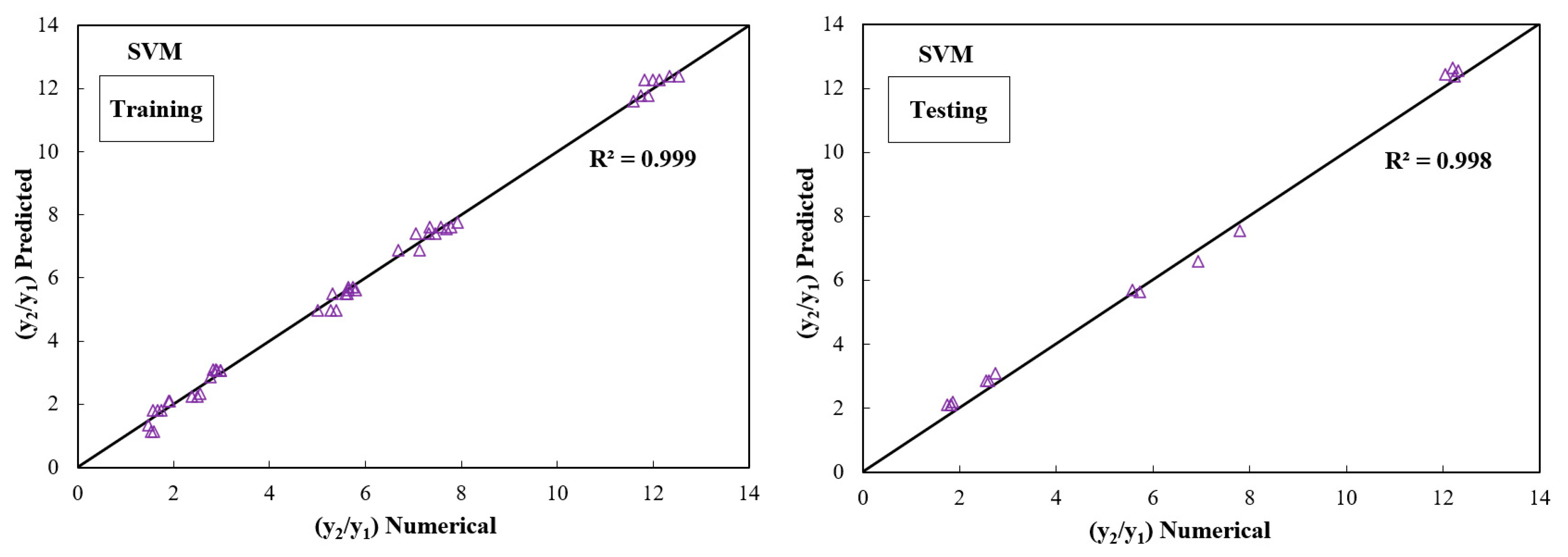
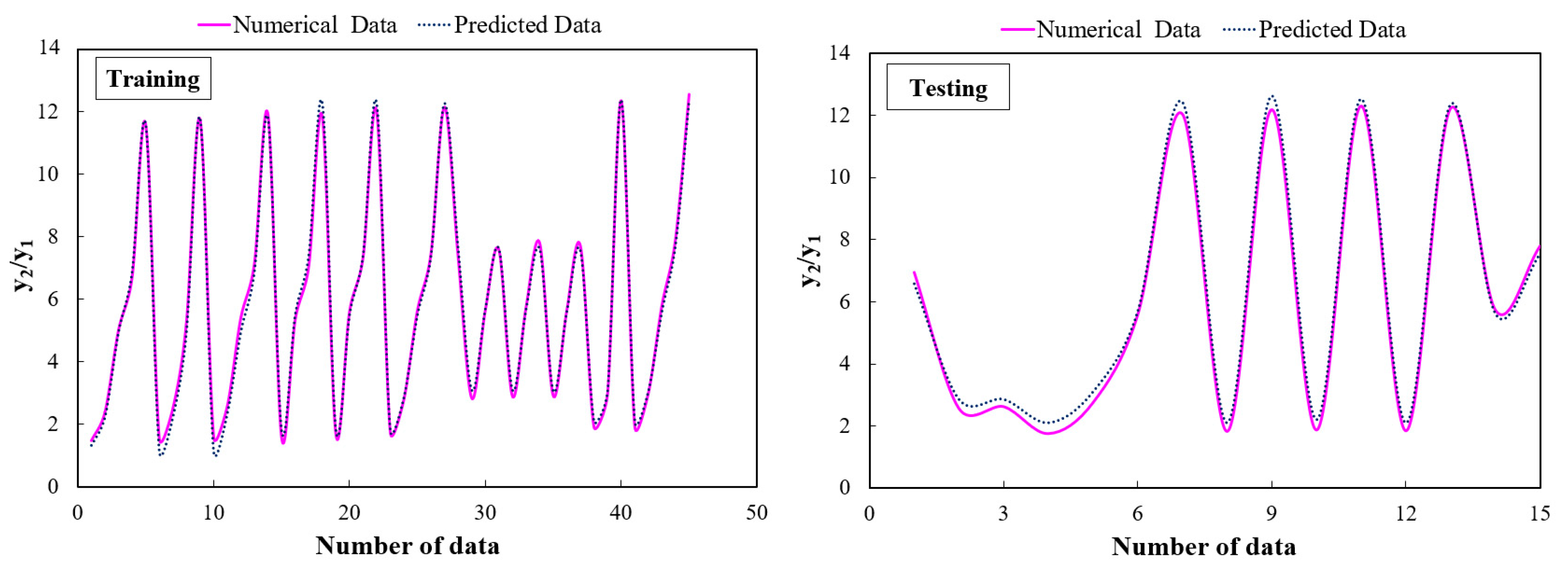
3.2. Sequent Depth Ratio in the Free Jump (y₂/y₁)

The y₂/y₁, which somehow represents the height of the jump, is directly related to the changes in the Fr₁ and the distance of the roughness element. By increasing these parameters, the value y₂/y₁ is increased. According to the results of the FLOW-3D^® model, the most significant decrease y₂/y₁ with increasing Froude number compared to the smooth bed is at T/I = 0.50 with 17.83% as mean. The results showed that the y₂/y₁ for the jump on the bed roughness was smaller than that of the corresponding jumps on a smooth bed [26,27].

Table 5. Prediction results for the sequent depth ratio (y₂/y₁).

Training					Testing
Model	R2	RMSE	NRMSE (%)	MAPE (%)	R2	RMSE	NRMSE (%)	MAPE (%)
GEP	0.9953	0.2356	4.03	5.35	0.9933	0.3335	5.56	8.83
RF	0.9682	0.5924	10.97	11.91	0.9275	1.0811	14.73	11.26
SVM	0.9966	0.2075	3.5481	5.07	0.9960	0.2990	4.98	8.46

summarizes the results of estimating the y₂/y₁. Comparing the results of three models, the SVM model with the lowest RMSE = 0.2075 and the highest R² = 0.9966 for the training phase and RMSE = 0.2990 and R² = 0.9960 for the testing phase in predicting the y₂/y₁ as a model the best was selected.

Figure 10 and Figure 11 compare the results of the FLOW-3D^® model and the SVM model to estimate the y₂/y₁ in the training and testing phase. It can be seen that the SVM model has a good performance in predicting this parameter, and the output results of the SVM model are in good agreement with the FLOW-3D^® values and were recognized as the best model. It is also observed that during predicting y₂/y₁ in the testing phase, the SVM model estimates higher values at maximum points than the FLOW-3D^® model.

In general, based on the numerical data of the present study, the equation provided for the y₂/y₁ in the free jump with a correlation coefficient equal to 0.997 is expressed as:

$$\frac{y_2}{y_1}=1.338F{r}_1-2.458(\frac{T}{I})+0.0528$$

(18)

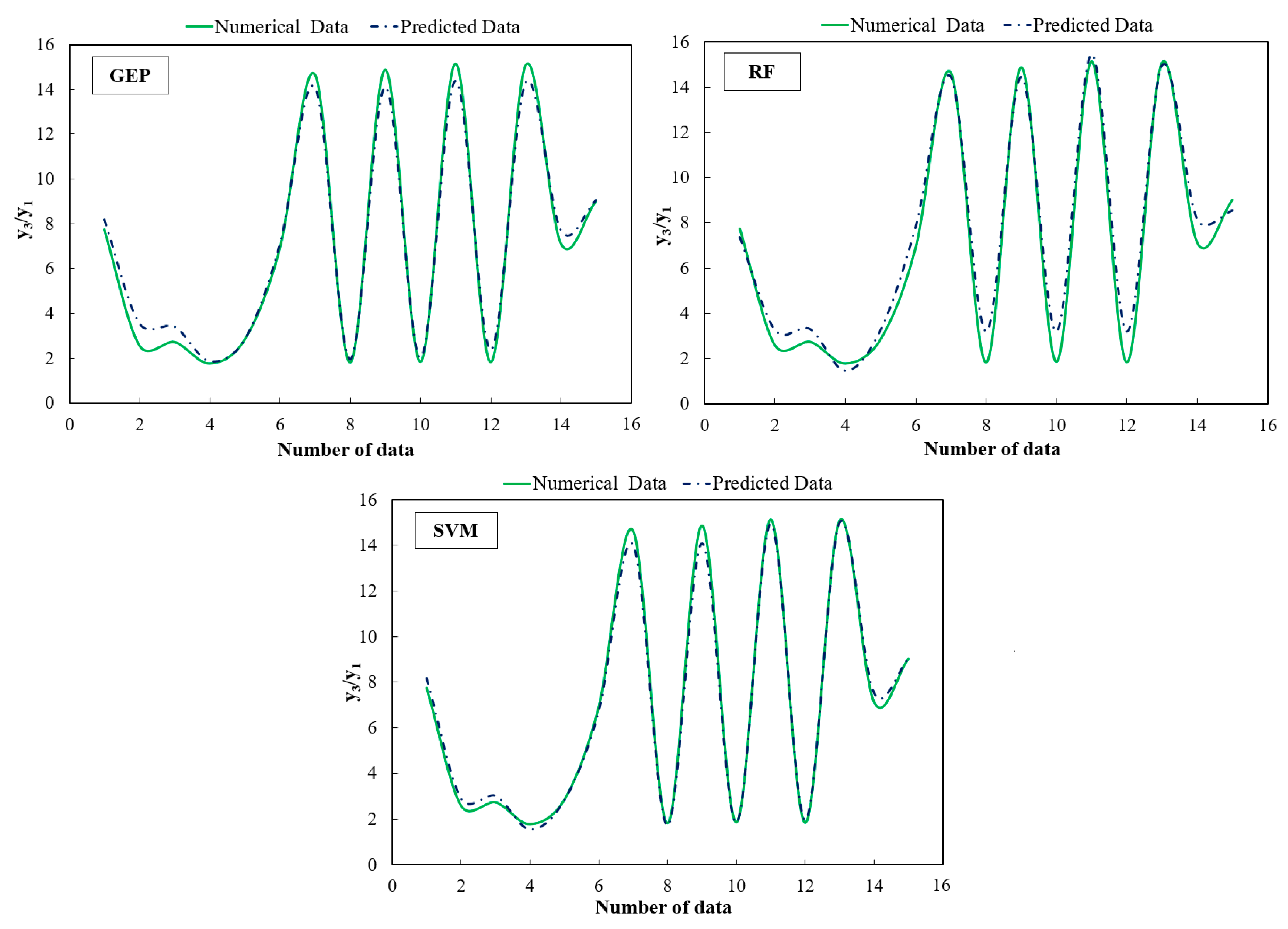
3.3. Submerged Depth Ratio in Submerged Jump (y₃/y₁)

Based on dimensional analysis, the submerged depth ratio (y₃/y₁) and the tailwater ratio (y₄/y₁) depend on the Fr₁, T/I, and SF. According to the results of the FLOW-3D^®, the most significant decrease y₃/y₁ and y₄/y₁ with increasing Froude number compared to the smooth bed are at T/I = 0.50 with 20.88% and 23.34% as mean, respectively [26,27]. Comparing the results of the three models presented in

Table 6. Prediction results for the submerged depth ratio (y₃/y₁) and the tailwater depth ratio (y₄/y₁).

Training					Testing
y3/y1	R2	RMSE	NRMSE (%)	MAPE (%)	R2	RMSE	NRMSE (%)	MAPE (%)
GEP	0.9903	0.4016	5.96	8.63	0.9895	0.5379	7.61	9.92
RF	0.9815	0.5679	8.43	11.97	0.9750	0.7804	11.04	23.03
SVM	0.9978	0.2024	3.01	2.67	0.9964	0.3391	4.80	4.93
y4/y1	R2	RMSE	NRMSE (%)	MAPE (%)	R2	RMSE	NRMSE (%)	MAPE (%)
GEP	0.9972	0.2811	3.41	3.34	0.9963	0.3923	4.54	6.84
RF	0.9901	0.5157	6.26	9.68	0.9899	0.6462	7.48	10.04
SVM	0.9991	0.1639	1.99	1.63	0.9988	0.2806	3.25	5.08

shows that among the three models, for the y₃/y₁, the SVM model with values of RMSE = 0.3391 and R² = 0.9964 for the testing phase is close to the FLOW-3D^® numerical model. The SVM model also performed better in predicting y₄/y₁ and had very little error. After the SVM model, the GEP model also provided acceptable results in estimating (y₃/y₁) and (y₄/y₁).

Figure 12 and Figure 13 present the results of comparing the FLOW-3D^® model and predicting the SVM, GEP, and RF models in the testing phase (y₃/y₁) and (y₄/y₁). According to the graphs, it is clear that the SVM model has a better prediction than the other two models. At the maximum and minimum points, the (y₃/y₁) and (y₄/y₁), always accompanied by turbulence in the water surface, it can be seen that the SVM model has the highest efficiency and the lowest error over other models. The predicted values of these parameters by the SVM model have good adaptation. They overlap with the output values of the numerical model.

In general, based on the results drawn from this study, the following equation for the y₃/y₁ and y₄/y₁ in the submerged jump with a correlation coefficient equal to 0.993 and 0.989, respectively, on the triangular bed roughness was obtained:

$$\frac{y_3}{y_1}=1.538F{r}_1+3.263SF-3.219(\frac{T}{I})-0.915$$

(19)

$$\frac{y_4}{y_1}=1.909F{r}_1+3.015SF-3.961(\frac{T}{I})-0.977$$

(20)

3.4. The Length Ratio of Jumps ($L_j$/$y_2^{*}$)

In the present study, the subcritical depth of the classical hydraulic jump ($y_2^{*}$) can be obtained by the Bélanger equation, as explained by French [57]:

$$y_2^{*}=\frac{y_1}{2}\left[\sqrt{(1+8F{r}_1^2)}-1\right]$$

(21)

According to the results of the FLOW-3D^® model, the ($L_j$/$y_2^{*}$) for the bed roughness is less than the smooth bed, and for the submerged jump it is larger than the free jump. For T/I = 0.5, the ratio length of free and submerged jumps decreases by about 25.52% and 21.65% as a mean, respectively [27]. Estimating the jump length reduces the volume of construction operations and ultimately reduces the project’s overall cost. Therefore, an accurate estimation of the hydraulic jump length is essential to design the length of the stilling basin based on this parameter. The results of predicting ($L_j$/$y_2^{*}$) along with the evaluation criteria are presented in

Table 7. Prediction results for the length of the jumps ($L_j/y_2^{*}$).

Training					Testing
$L_{jf}$/$y_2^{*}$	R2	RMSE	NRMSE (%)	MAPE (%)	R2	RMSE	NRMSE (%)	MAPE (%)
GEP	0.829	0.234	4.39	3.66	0.766	0.249	4.54	4.54
RF	0.752	0.278	5.08	3.92	0.741	0.319	6.32	5.21
SVM	0.919	0.169	3.16	2.74	0.881	0.174	3.19	2.90
$L_{js}$/$y_2^{*}$	R2	RMSE	NRMSE (%)	MAPE%	R2	RMSE	NRMSE (%)	MAPE (%)
GEP	0.878	0.273	3.88	3.17	0.867	0.336	4.71	4.33
RF	0.787	0.316	4.37	3.51	0.764	0.425	6.50	5.46
SVM	0.961	0.154	2.19	1.93	0.940	0.212	2.97	2.37

. According to the results, the SVM model has good statistical criteria among other models and has high accuracy in predicting the relative length of free and submerged hydraulic jumps.

Graphs of changes in R² and RMSE versus different gammas are presented for the best model of the $L_{jf}$/$y_2^{*}$ and the $L_{js}$/$y_2^{*}$ in the testing phase (Figure 14). In the support vector machine, selecting the appropriate gamma is one of the main parameters in determining the best model, which has been done by trial and error. Finally, the best result for predicting the $L_{jf}$/$y_2^{*}$ in the optimal gamma is 10 (γ = 10), and for $L_{js}$/$y_2^{*}$ in the optimal gamma it is 0.60 (γ = 0.60).

Figure 15 and Figure 16 show the results of the FLOW-3D^® and the predicted models of $L_{jf}$/$y_2^{*}$ and the $L_{js}$/$y_2^{*}$ data for the best SVM model in the training and testing phases. According to Figure 15, it can be seen that when the values of the $L_{jf}$/$y_2^{*}$ reach the maximum and minimum points, the prediction accuracy of the SVM model decreases. In other words, when the $L_{jf}$/$y_2^{*}$ reaches the maximum and minimum jump values, the prediction error of the SVM model increases. Moreover, as shown in Figure 16 for the $L_{js}$/$y_2^{*}$, it can be seen that the SVM model always has values close to the FLOW-3D^® model and has a better performance compared to the $L_{jf}$/$y_2^{*}$. On the other hand, most SVM model errors in both parameters occurred in the initial range of testing data. In the middle to the end of the data, the prediction error decreased.

The following equation shows the relationship between the $L_j$/$y_2^{*}$ with a correlation coefficient equal to 0.724 and 0.944, respectively, for the free and submerged jumps:

$$\frac{L_{jf}}{y_2^{*}}=0.065F{r}_1-3.757(\frac{T}{I})+6.103$$

(22)

$$\frac{L_{js}}{y_2^{*}}=0.037F{r}_1+5.568SF-2.556(\frac{T}{I})+5.579$$

(23)

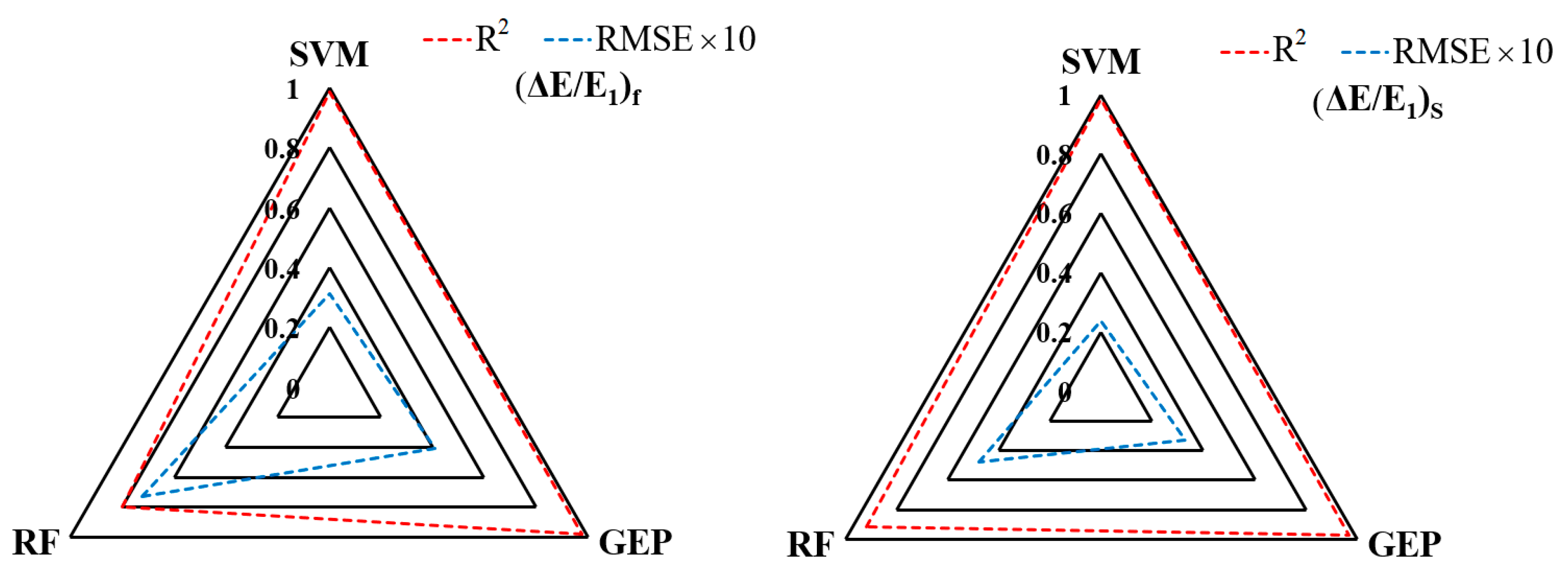
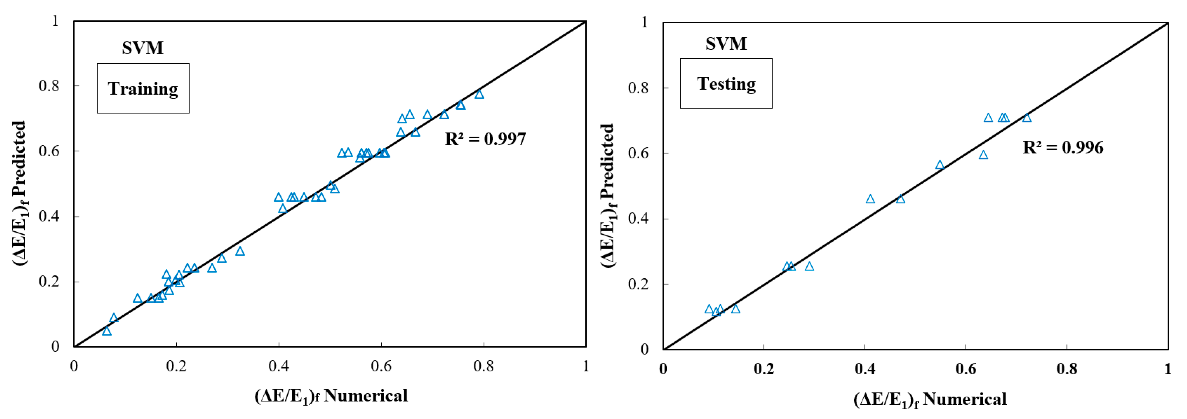
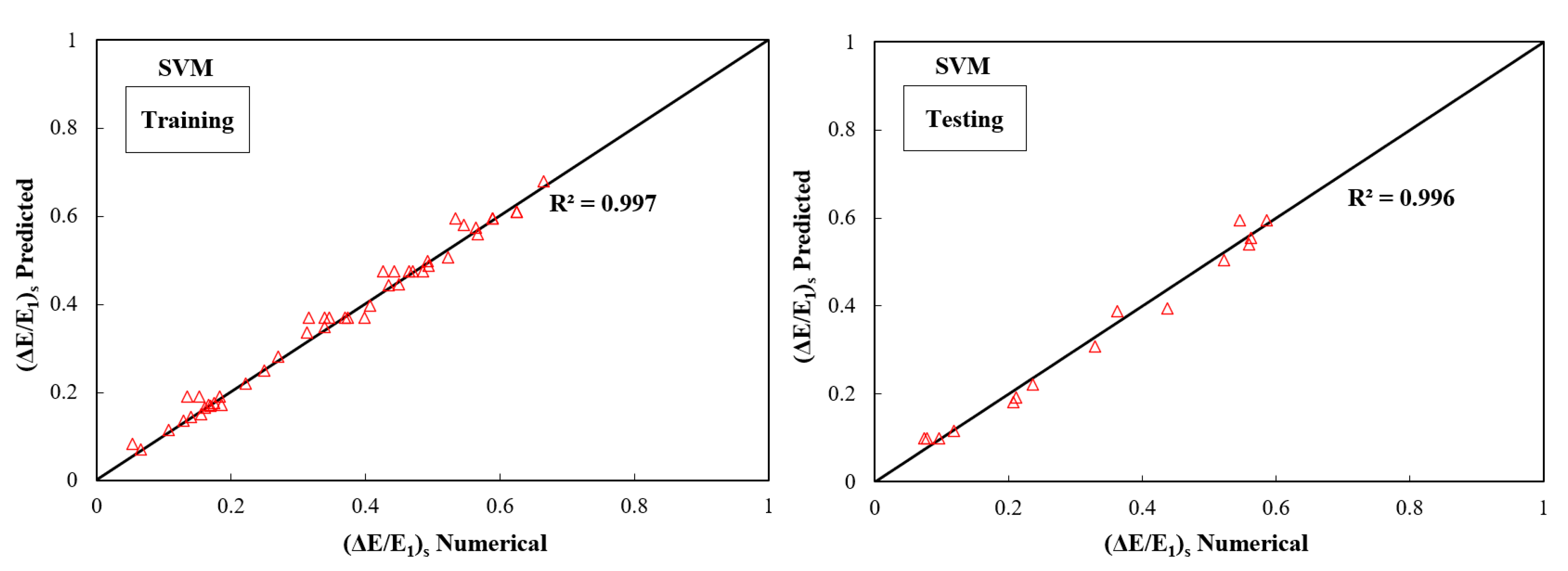
3.5. The Energy Dissipation (ΔE/E₁)

The energy dissipation of hydraulic jumps based on free and submerged is calculated as follows by Pourabdollah et al. [17]:

$${(\frac{\Delta E}{E_1})}_f={(\frac{E_1-E_2}{E_1})}_f={(\frac{(y_1+V_1^2/2g)-(y_2+V_2^2/2g)}{y_1+V_1^2/2g})}_f$$

(24)

$${(\frac{\Delta E}{E_1})}_s={(\frac{E_3-E_4}{E_3})}_s={(\frac{(y_3+V_1^2/2g)-(y_4+V_4^2/2g)}{y_3+V_1^2/2g})}_s$$

(25)

E₁, E₂, E₃, and E₄ are specific energies upstream and downstream of the free and submerged jumps, respectively (see Figure 1). According to the results of the FLOW-3D^®, the ΔE/E₁ increases with increasing the Fr₁. The highest ΔE/E₁ occurs with T/I = 0.50 in the free and submerged jumps compared to other distances between the roughnesses of the corresponding T/I ratios [26,27]. Determining the amount of ΔE/E₁ that occurs due to hydraulic jumps will lead to the stilling basin’s more efficient and economical design. The results of predicting energy dissipation due to free jump (ΔE/E₁)_f and submerged jump (ΔE/E₁)_S are presented in

Table 8. Prediction results for the energy dissipation (ΔE/E₁).

Training					Testing
(ΔE/E1)f	R2	RMSE	NRMSE (%)	MAPE (%)	R2	RMSE	NRMSE (%)	MAPE (%)
GEP	0.980	0.029	6.76	6.59	0.977	0.040	10.19	16.04
RF	0.855	0.069	16.5	25.61	0.801	0.072	16.32	21.22
SVM	0.985	0.027	6.37	6.58	0.984	0.031	7.80	9.04
(ΔE/E1)S	R2	RMSE	NRMSE (%)	MAPE (%)	R2	RMSE	NRMSE (%)	MAPE (%)
GEP	0.980	0.025	7.22	8.85	0.969	0.033	10.07	11.63
RF	0.912	0.051	12.94	13.83	0.916	0.047	13.53	13.43
SVM	0.985	0.022	6.22	6.43	0.984	0.023	7.25	9.05

. The results showed that for energy dissipation for (ΔE/E₁)_f, the SVM model with R² = 0.9848 and RMSE = 0.0313, and for the testing phase (ΔE/E₁)_S, R² = 0.9843 and RMSE = 0.0238, these were recognized as the best models. Therefore, the best prediction with the least possible error among the three models is obtained by the SVM model.

Two radar graphs of the R² and RMSE of energy dissipation due to free and submerged jumps are presented for the testing phase (Figure 17). Radar graphs can show the accuracy of predictions of different models compared to each other. It can be seen that the SVM model has provided acceptable performance and has a much better prediction than the GEP and RF models. Furthermore, because RMSE values are small and their changes are not visible in the graph, by multiplying the RMSE by 10, the range of changes became broader and more precise.

The distribution graph between numerical and predicted values is plotted for the best energy dissipation model due to free and submerged jumps (Figure 18 and Figure 19). Changes in energy dissipation for jumps during the testing and training phase indicate good agreement and overlap between the values of the numerical model and the predicted. According to the figure, it can be seen that the data of the numerical model had less dispersion with the predicted data. In other words, the output data are very well matched to each other. Additionally, during the model simulation process, the network training did not fail, and the training values were always higher than the testing.

The following equations show the relationship between the ΔE/E₁ and Fr₁ with a correlation coefficient equal to 0.963 and 0.946, respectively, for the free and submerged jumps:

$${(\frac{\Delta E}{E_1})}_f=-0.009F{r}_1^2+0.184F{r}_1-0.177$$

(26)

$${(\frac{\Delta E}{E_1})}_s=-0.007F{r}_1^2+0.146F{r}_1-0.143$$

(27)

3.6. Sensitivity Analysis

Sensitivity analysis is the best solution to achieve the effectiveness of the input variables of a statistical model in a study. Sensitivity analysis is used when sufficient inputs are changed in an organized statistical model to observe the effects of the presence or absence of these variables in the predictive output model. The present study omitted the one-by-one parameters to predict the submerged depth ratio (y₃/y₁). The parameter that had the most impact was identified, and its results are presented in

Table 9. Sensitivity analysis results for the submerged depth ratio (y₃/y₁).

Training						Testing
Input parameter	Omitted parameter	R2	RMSE	NRME (%)	MAPE (%)	R2	RMSE	NRMSE (%)	MAPE (%)
Fr1, SF, T/I	-	0.999	0.163	1.99	1.63	0.998	0.280	3.25	5.08
SF, T/I	Fr1	0.787	1.639	24.33	34.63	0.731	2.417	34.21	36.69
Fr1, T/I	SF	0.986	0.479	7.12	10.83	0.984	0.664	9.41	15.9
Fr1, SF	T/I	0.989	0.415	6.17	9.85	0.988	0.548	7.76	14.66

.

It can be seen that the best result for predicting the effective parameter of (y₃/y₁) is when all three parameters of Fr₁, T/I, and SF are involved in the prediction. The Fr₁ has the greatest effect on predicting the (y₃/y₁) based on sensitivity analysis. By omitting this parameter, the prediction accuracy is significantly reduced. The SF and T/I are also involved in the study of (y₃/y₁), but the impact of each is less than the Fr₁.

4. Conclusions

This paper presented and discussed the characteristics of free and submerged hydraulic jumps on the triangular bed roughness in various roughness arrangements of the corresponding T/I ratios with the CFD techniques and compared the prediction of this numerical model with the help of artificial intelligence methods (SVM, GEP, and RF). To simulate the free flow surface, the Volume of Fluid (VOF) method, and the turbulence, the RNG k-ε model in FLOW-3D^® software was used. Key findings of the comparative analysis are given below:

• By comparing the results of the two experiments (physical and numerical), the FLOW-3D^® software can accurately predict the characteristics of free and submerged hydraulic jumps. The overall mean value of relative error between numerical results and experimental data is 4.1%, which confirms the numerical model’s ability to predict the characteristics of the free and submerged jumps.
• The SVM model with the RMSE = 0.2075 and R² = 0.9966 for the training phase and RMSE = 0.2990 and R² = 0.9960 for the testing phase in predicting the y₂/y₁ is the best model and close to the FLOW-3D^® result.
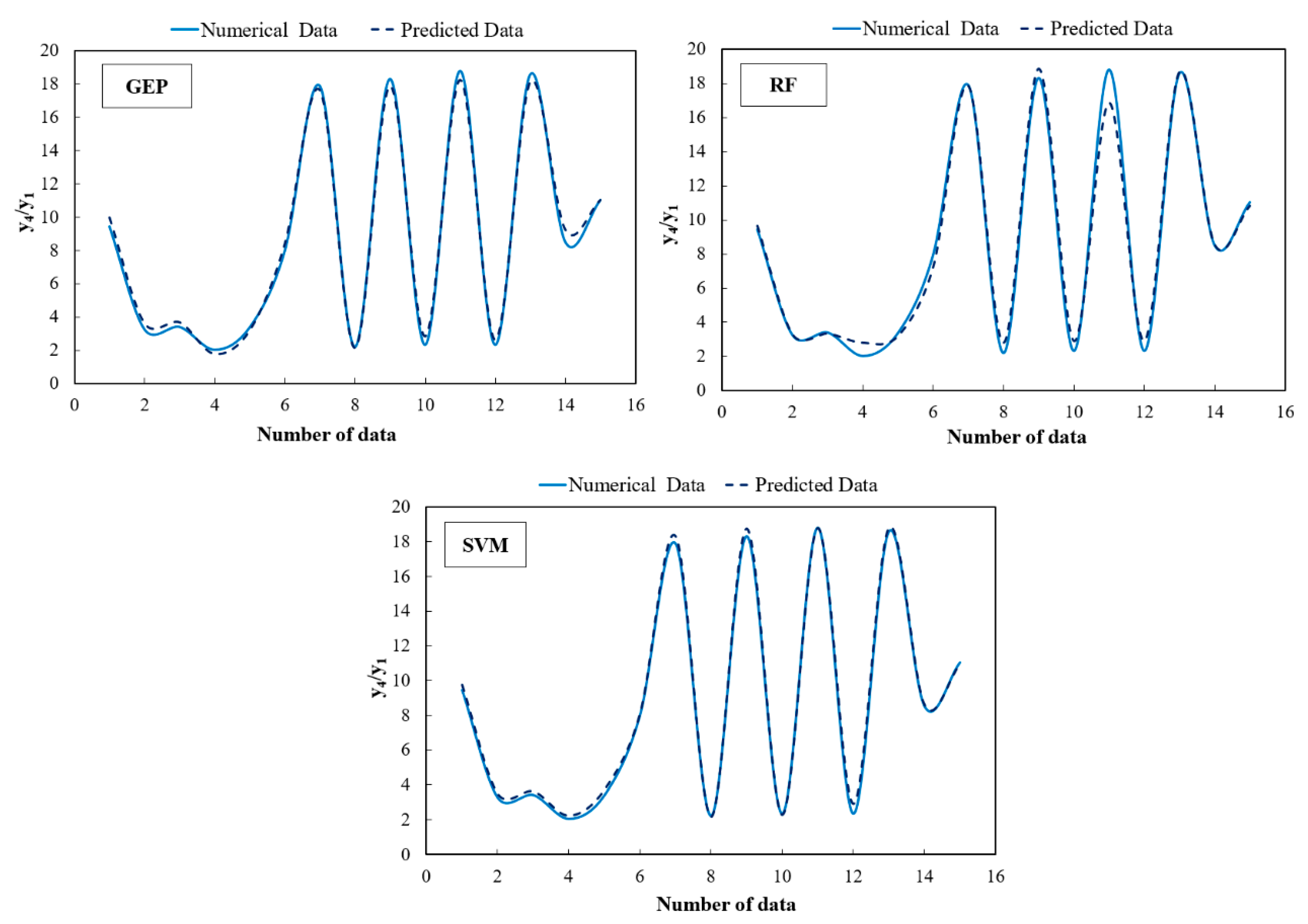
• For the y₃/y₁, the SVM model with values of RMSE = 0.3391 and R² = 0.9964 for the testing phase is close to the FLOW-3D^® model. The SVM model also performed better in predicting y₄/y₁ and had very little error. After the SVM model, the GEP model also provided acceptable results in estimating (y₃/y₁) and (y₄/y₁).
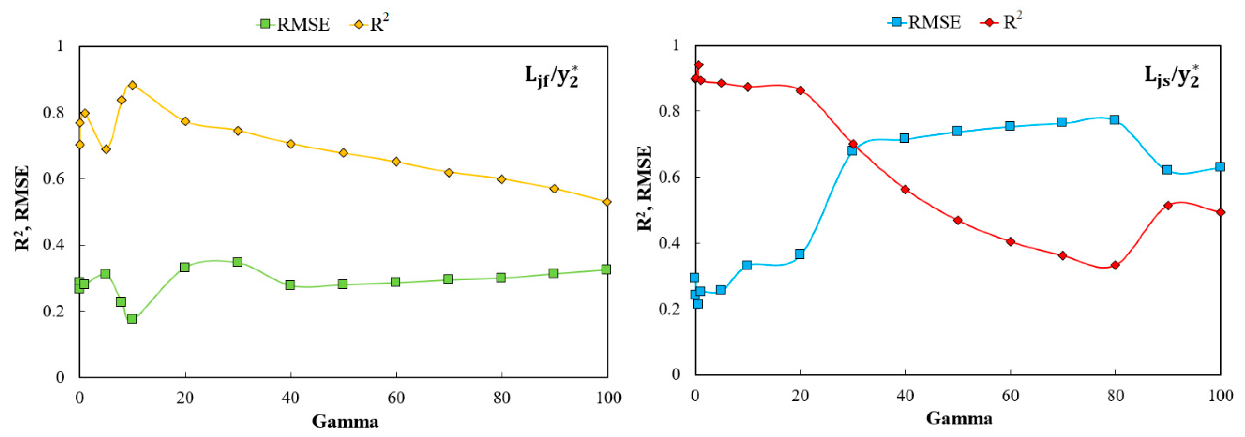
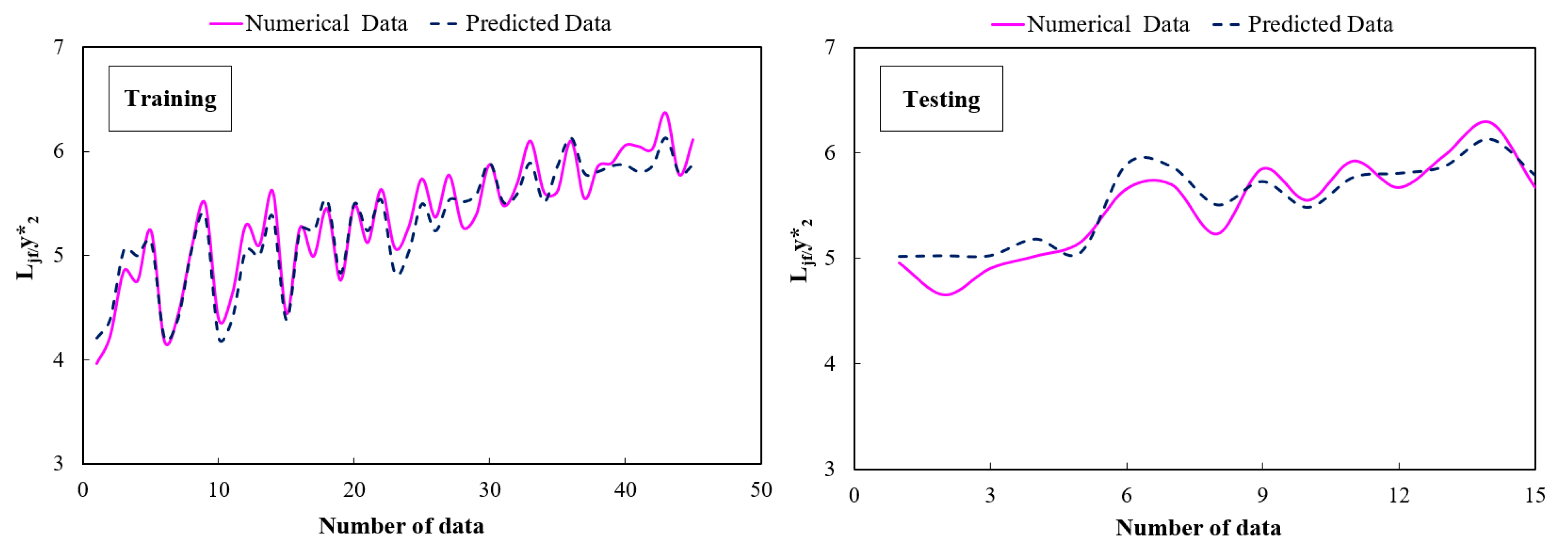
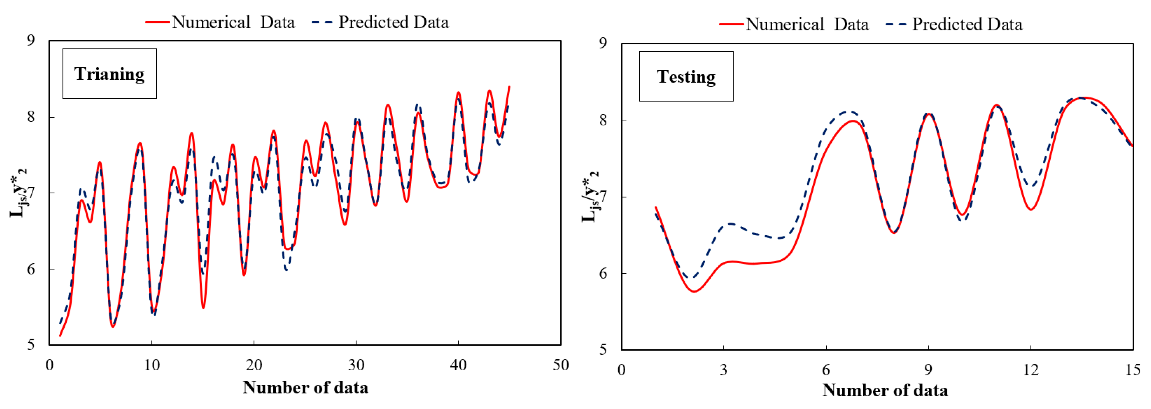
• The SVM model demonstrated better statistical criteria among other models (i.e., GEP and RF) and has high accuracy in predicting the relative length of free and submerged hydraulic jumps. Furthermore, the best result for predicting the $L_{jf}/y_2^{*}$ in the optimal gamma is 10 (γ = 10) and the $L_{js}/y_2^{*}$ in the optimal gamma is 0.60 (γ = 0.60).
• For energy dissipation due to (ΔE/E₁)_f and (ΔE/E₁)_S, for the testing phase, SVM model with R² = 0.9848 and RMSE = 0.031 as well as R² = 0.9843 and RMSE = 0.0238 were recognized as the best models, respectively.
• The Fr₁ has the greatest effect on predicting the (y₃/y₁) based on sensitivity analysis. By omitting this parameter, the prediction accuracy is significantly reduced. The SF and T/I are also involved in the (y₃/y₁), but the impact of each is less than the Fr₁.
• Relationships with good correlation coefficients for the mentioned parameters in free and submerged hydraulic jumps were presented based on numerical results.

Finally, the methodology presented in this study and the solution-oriented result contributes to helping hydraulic engineers to design and construct cost-effective spillways, stilling basins, and other hydraulic structures that experience hydraulic jumps. Indeed, the accurate estimation of the hydraulic jump length, especially in high head spillways, reduces construction operations’ volume and ultimately reduces the project’s overall cost of the stilling basin built to dissipate the hydraulic jumps.

References

1. Ebrahimi, S.; Salmasi, F.; Abbaspour, A. Numerical study of hydraulic jump on rough beds stilling basins. J. Civ. Eng. Urban. 2013, 3, 19–24. [Google Scholar]
2. Chanson, H. Hydraulics of Open Channel Flow; Elsevier: Amsterdam, The Netherlands, 2004. [Google Scholar]
3. McCorquodale, J.A.; Khalifa, A.M. Submerged radial hydraulic jump. J. Hydraul. Div. 1980, 106, 355–367. [Google Scholar] [CrossRef]
4. Smith, C.D. The submerged hydraulic jump in an abrupt lateral expansion. J. Hydraul. Res. 1989, 27, 257–266. [Google Scholar] [CrossRef]
5. Graber, S.D.; Ohtsu, I.; Yasuda, Y.; Ishikawa, M. Submerged Hydraulic Jumps below Abrupt Expansions. J. Hydraul. Eng. 2001, 127, 84–85. [Google Scholar] [CrossRef]
6. Vallé, B.L.; Pasternack, G.B. Submerged and unsubmerged natural hydraulic jumps in a bedrock step-pool mountain channel. Geomorphology 2006, 82, 146–159. [Google Scholar] [CrossRef]
7. Dey, S.; Sarkar, A. Characteristics of turbulent flow in submerged jumps on rough beds. J. Eng. Mech. 2008, 134, 49–59. [Google Scholar] [CrossRef]
8. Tokyay, N.; Evcimen, T.; Şimşek, Ç. Forced hydraulic jump on non-protruding rough beds. Can. J. Civ. Eng. 2011, 38, 1136–1144. [Google Scholar] [CrossRef]
9. Samadi-Boroujeni, H.; Ghazali, M.; Gorbani, B.; Nafchi, R.F. Effect of triangular corrugated beds on the hydraulic jump characteristics. Can. J. Civ. Eng. 2013, 40, 841–847. [Google Scholar] [CrossRef]
10. Ead, S.; Rajaratnam, N. Hydraulic jumps on corrugated beds. J. Hydraul. Eng. 2002, 128, 656–663. [Google Scholar] [CrossRef]
11. Carollo, F.G.; Ferro, V.; Pampalone, V. Hydraulic jumps on rough beds. J. Hydraul. Eng. 2007, 133, 989–999. [Google Scholar] [CrossRef]
12. Pagliara, S.; Lotti, I.; Palermo, M. Hydraulic jump on rough bed of stream rehabilitation structures. J. Hydro-Environ. Res. 2008, 2, 29–38. [Google Scholar] [CrossRef]
13. Abbaspour, A.; Hosseinzadeh Dalir, A.; Farsadizadeh, D.; Sadraddini, A.A. Effect of sinusoidal corrugated bed on hydraulic jump characteristics. J. Hydro-Environ. Res. 2009, 3, 109–117. [Google Scholar] [CrossRef]
14. Chanson, H. Momentum considerations in hydraulic jumps and bores. J. Irrig. Drain. Eng. 2012, 138, 382–385. [Google Scholar] [CrossRef] [Green Version]
15. Ahmed, H.M.A.; El Gendy, M.; Mirdan, A.M.H.; Ali, A.A.M.; Haleem, F.S.F.A. Effect of corrugated beds on characteristics of submerged hydraulic jump. Ain Shams Eng. J. 2014, 5, 1033–1042. [Google Scholar] [CrossRef] [Green Version]
16. Palermo, M.; Pagliara, S. Semi-theoretical approach for energy dissipation estimation at hydraulic jumps in rough sloped channels. J. Hydraul. Res. 2018, 56, 786–795. [Google Scholar] [CrossRef]
17. Pourabdollah, N.; Heidarpour, M.; Koupai, J.A. Characteristics of free and submerged hydraulic jumps in different stilling basins. Water Manag. 2020, 173, 121–131. [Google Scholar] [CrossRef]
18. Habibzadeh, A.; Rajaratnam, N.; Loewen, M. Characteristics of the flow field downstream of free and submerged hydraulic jumps. Water Manag. 2019, 172, 180–194. [Google Scholar] [CrossRef]
19. Gharangik, A.M.; Chaudhry, M.H. Numerical simulation of hydraulic jump. J. Hydraul. Eng. 1991, 117, 1195–1211. [Google Scholar] [CrossRef]
20. Ma, F.; Hou, Y.; Prinos, P. Numerical calculation of submerged hydraulic jumps. J. Hydraul. Res. 2001, 39, 493–503. [Google Scholar] [CrossRef]
21. Mousavi, S.N.; Júnior, R.S.; Teixeira, E.D.; Bocchiola, D.; Nabipour, N.; Mosavi, A.; Shamshirband, S. Predictive Modeling the Free Hydraulic Jumps Pressure through Advanced Statistical Methods. Mathematics 2020, 8, 323. [Google Scholar] [CrossRef] [Green Version]
22. Abbaspour, A.; Farsadizadeh, D.; Dalir, A.H.; Sadraddini, A.A. Numerical study of hydraulic jumps on corrugated beds using turbulence models. Turk. J. Eng. Environ. Sci. 2009, 33, 61–72. [Google Scholar]
23. Chern, M.-J.; Syamsuri, S. Effect of corrugated bed on hydraulic jump characteristic using SPH method. J. Hydraul. Eng. 2013, 139, 221–232. [Google Scholar] [CrossRef]
24. Bayon, A.; Valero, D.; García-Bartual, R.; Vallés-Morán, F.J.; López-Jiménez, P.A. Performance assessment of OpenFOAM and FLOW-3D in the numerical modeling of a low Reynolds number hydraulic jump. Environ. Model. Softw. 2016, 80, 322–335. [Google Scholar] [CrossRef]
25. Nikmehr, S.; Aminpour, Y. Numerical Simulation of Hydraulic Jump over Rough Beds. Period. Polytech. Civ. Eng. 2020, 64, 396–407. [Google Scholar] [CrossRef]
26. Ghaderi, A.; Dasineh, M.; Aristodemo, F.; Ghahramanzadeh, A. Characteristics of free and submerged hydraulic jumps over different macroroughnesses. J. Hydroinform. 2020, 22, 1554–1572. [Google Scholar] [CrossRef]
27. Ghaderi, A.; Dasineh, M.; Aristodemo, F.; Aricò, C. Numerical Simulations of the Flow Field of a Submerged Hydraulic Jump over Triangular Macroroughnesses. Water 2021, 13, 674. [Google Scholar] [CrossRef]
28. Karbasi, M.; Azamathulla, H.M. GEP to predict characteristics of a hydraulic jump over a rough bed. KSCE J. Civ. Eng. 2016, 20, 3006–3011. [Google Scholar] [CrossRef]
29. Roushangar, K.; Ghasempour, R. Explicit prediction of expanding channels hydraulic jump characteristics using gene expression programming approach. Hydrol. Res. 2017, 49, 815–830. [Google Scholar] [CrossRef]
30. Roushangar, K.; Ghasempour, R. Evaluation of the impact of channel geometry and rough elements arrangement in hydraulic jump energy dissipation via SVM. J. Hydroinform. 2018, 21, 92–103. [Google Scholar] [CrossRef]
31. Roushangar, K.; Homayounfar, F. Prediction Characteristics of Free and Submerged Hydraulic Jumps on Horizontal and Sloping Beds using SVM Method. KSCE J. Civ. Eng. 2019, 23, 4696–4709. [Google Scholar] [CrossRef]
32. Naseri, M.; Othman, F. Determination of the length of hydraulic jumps using artificial neural networks. Adv. Eng. Softw. 2012, 48, 27–31. [Google Scholar] [CrossRef]
33. Nasrabadi, M.; Mehri, Y.; Ghassemi, A.; Omid, M.H. Predicting submerged hydraulic jump characteristics using machine learning methods. Water Supply 2021. [Google Scholar] [CrossRef]
34. Huš, M.; Grilc, M.; Pavlišič, A.; Likozar, B.; Hellman, A. Multiscale modelling from quantum level to reactor scale: An example of ethylene epoxidation on silver catalysts. Catal. Today 2019, 338, 128–140. [Google Scholar] [CrossRef]
35. Hager, W.H.; Bremen, R. Classical hydraulic jump: Sequent depths. J. Hydraul. Res. 1989, 27, 565–585. [Google Scholar] [CrossRef]
36. Fürst, J.; Halada, T.; Sedlář, M.; Krátký, T.; Procházka, P.; Komárek, M. Numerical Analysis of Flow Phenomena in Discharge Object with Siphon Using Lattice Boltzmann Method and CFD. Mathematics 2021, 9, 1734. [Google Scholar] [CrossRef]
37. Hirt, C.W.; Nichols, B.D. Volume of fluid (VOF) method for the dynamics of free boundaries. J. Comput. Phys. 1981, 39, 201–225. [Google Scholar] [CrossRef]
38. Nazari-Sharabian, M.; Nazari-Sharabian, A.; Karakouzian, M.; Karami, M. Sacrificial piles as scour countermeasures in river bridges a numerical study using flow-3D. Civ. Eng. J. 2020, 6, 1091–1103. [Google Scholar] [CrossRef]
39. Abbasi, S.; Fatemi, S.; Ghaderi, A.; Di Francesco, S. The Effect of Geometric Parameters of the Antivortex on a Triangular Labyrinth Side Weir. Water 2021, 13, 14. [Google Scholar] [CrossRef]
40. Chiu, C.-L.; Fan, C.-M.; Tsung, S.-C. Numerical Modeling for Periodic Oscillation of Free Overfall in a Vertical Drop Pool. J. Hydraul. Eng. 2017, 143, 04016077. [Google Scholar] [CrossRef]
41. Wang, Y.; Wang, W.; Hu, X.; Liu, F. Experimental and numerical research on trapezoidal sharp-crested side weirs. Flow Meas. Instrum. 2018, 64, 83–89. [Google Scholar] [CrossRef]
42. Ghaderi, A.; Daneshfaraz, R.; Dasineh, M.; Di Francesco, S. Energy dissipation and hydraulics of flow over trapezoidal–triangular labyrinth weirs. Water 2020, 12, 1992. [Google Scholar] [CrossRef]
43. Ghaderi, A.; Abbasi, S. CFD simulation of local scouring around airfoil-shaped bridge piers with and without collar. Sādhanā 2019, 44, 216. [Google Scholar] [CrossRef] [Green Version]
44. Ghaderi, A.; Dasineh, M.; Abbasi, S.; Abraham, J. Investigation of trapezoidal sharp-crested side weir discharge coefficients under subcritical flow regimes using CFD. Appl. Water Sci. 2019, 10, 31. [Google Scholar] [CrossRef] [Green Version]
45. Ghaderi, A.; Abbasi, S.; Abraham, J.; Azamathulla, H.M. Efficiency of Trapezoidal Labyrinth Shaped stepped spillways. Flow Meas. Instrum. 2020, 72, 101711. [Google Scholar] [CrossRef]
46. Daneshfaraz, R.; Aminvash, E.; Ghaderi, A.; Abraham, J.; Bagherzadeh, M. SVM Performance for Predicting the Effect of Horizontal Screen Diameters on the Hydraulic Parameters of a Vertical Drop. Appl. Sci. 2021, 11, 4238. [Google Scholar] [CrossRef]
47. Daneshfaraz, R.; Bagherzadeh, M.; Esmaeeli, R.; Norouzi, R.; Abraham, J. Study of the performance of support vector machine for predicting vertical drop hydraulic parameters in the presence of dual horizontal screens. Water Supply 2021, 21, 217–231. [Google Scholar] [CrossRef]
48. Thakur, B.; Kalra, A.; Ahmad, S.; Lamb, K.W.; Lakshmi, V. Bringing statistical learning machines together for hydro-climatological predictions—Case study for Sacramento San joaquin River Basin, California. J. Hydrol. Reg. Stud. 2020, 27, 100651. [Google Scholar] [CrossRef]
49. Roushangar, K.; Koosheh, A. Evaluation of GA-SVR method for modeling bed load transport in gravel-bed rivers. J. Hydrol. 2015, 527, 1142–1152. [Google Scholar] [CrossRef]
50. Roushangar, K.; Alami, M.T.; Shiri, J.; Asl, M.M. Determining discharge coefficient of labyrinth and arced labyrinth weirs using support vector machine. Hydrol. Res. 2017, 49, 924–938. [Google Scholar] [CrossRef]
51. Ferreira, C. Gene Expression Programming in Problem Solving. In Soft Computing and Industry: Recent Applications; Roy, R., Köppen, M., Ovaska, S., Furuhashi, T., Hoffmann, F., Eds.; Springer: London, UK, 2002; pp. 635–653. [Google Scholar]
52. Borrelli, A.; De Falco, I.; Della Cioppa, A.; Nicodemi, M.; Trautteur, G. Performance of genetic programming to extract the trend in noisy data series. Phys. A Stat. Mech. Its Appl. 2006, 370, 104–108. [Google Scholar] [CrossRef]
53. Majedi-Asl, M.; Daneshfaraz, R.; Fuladipanah, M.; Abraham, J.; Bagherzadeh, M. Simulation of bridge pier scour depth base on geometric characteristics and field data using support vector machine algorithm. J. Appl. Res. Water Wastewater 2020, 7, 137–143. [Google Scholar]
54. Antoniadis, A.; Lambert-Lacroix, S.; Poggi, J.-M. Random forests for global sensitivity analysis: A selective review. Reliab. Eng. Syst. Saf. 2021, 206, 107312. [Google Scholar] [CrossRef]
55. Pavlišič, A.; Pohar, A.; Likozar, B. Comparison of computational fluid dynamics (CFD) and pressure drop correlations in laminar flow regime for packed bed reactors and columns. Powder Technol. 2018, 328, 130–139. [Google Scholar] [CrossRef]
56. Pavlišič, A.; Huš, M.; Prašnikar, A.; Likozar, B. Multiscale modelling of CO2 reduction to methanol over industrial Cu/ZnO/Al2O3 heterogeneous catalyst: Linking ab initio surface reaction kinetics with reactor fluid dynamics. J. Clean. Prod. 2020, 275, 122958. [Google Scholar] [CrossRef]
57. French, R.H. Open-Channel Hydraulics; McGraw-Hill: New York, NY, USA, 1985. [Google Scholar]
Figure 1. Definition sketch of the free and submerged hydraulic jumps on a triangular bed roughness after Ghaderi et al. [26].
Mathematics 09 03135 g001
Figure 2. The boundary conditions governing the simulation, (a) smooth bed, (b) the triangular bed roughness.
Mathematics 09 03135 g002
Figure 3. CFD flow discharge time variation in the inlet and outlet boundaries, (a) Q = 0.03 m3/s, (b) Q = 0.045 m3/s.
Mathematics 09 03135 g003
Figure 4. Structured rectangular hexahedral mesh with two different mesh blocks, (a) smooth bed, (b) the triangular bed roughness.
Mathematics 09 03135 g004
Figure 5. Variations of the relative error of y3/y1 and y2/y1 at Fr1 versus cell size.
Mathematics 09 03135 g005
Figure 6. Schematic of the Support Vector Machine (SVM).
Mathematics 09 03135 g006
Figure 7. Schematic of the Gene Expression Programming (GEP).
Mathematics 09 03135 g007
Figure 8. Performance of Random Forest (RF).
Mathematics 09 03135 g008
Figure 9. Numerical versus basic experimental parameters of submerged and free hydraulic jumps. (a) y3/y1, (b) y4/y1, (c) Ljs/y1, and (d) y2/y1.
Mathematics 09 03135 g009
Figure 10. FLOW-3D® model versus SVM model predicted for the y2/y1.
Mathematics 09 03135 g010
Figure 11. Comparison of FLOW-3D® model and SVM model for estimating the y2/y1.
Mathematics 09 03135 g011
Figure 12. Comparison of the numerical results and the predicted models of (y3/y1) for the testing phase.
Mathematics 09 03135 g012
Figure 13. Comparison of the numerical results and the predicted models of (y4/y1) for the testing phase.
Mathematics 09 03135 g013
Figure 14. Variations R2 and RMSE versus gamma for the best SVM model in jump length estimation.
Mathematics 09 03135 g014
Figure 15. Comparison of FLOW-3D® and SVM model values to estimate the L j f / y 2 * .
Mathematics 09 03135 g015
Figure 16. Comparison of FLOW-3D® and SVM model values to estimate the L j s / y 2 * .
Mathematics 09 03135 g016
Figure 17. Radar graphs of R2 and RMSE for energy dissipation due to free and submerged jumps in the testing phase.
Mathematics 09 03135 g017
Figure 18. FLOW-3D® model versus SVM predicted for the free jump.
Mathematics 09 03135 g018
Figure 19. FLOW-3D® model versus SVM predicted for the submerged jump.
Mathematics 09 03135 g019