Article

Enterprise Compensation System Statistical Modeling for Decision Support System Development

1
Faculty of Control Systems, Tomsk State University of Control Systems and Radioelectronics, 634050 Tomsk, Russia
2
Department of Experimental Physics, Tomsk Polytechnic University, 634050 Tomsk, Russia
*
Author to whom correspondence should be addressed.
Mathematics 2021, 9(23), 3126; https://doi.org/10.3390/math9233126
Submission received: 31 October 2021 / Revised: 26 November 2021 / Accepted: 28 November 2021 / Published: 4 December 2021

Abstract

:
This article raises the issue of decision support system (DSS) development in enterprises concerning the compensation system (CS). The topic is relevant as the CS is one of the main components in human resource management in business. A key element of such DSSs is CS models that provide predictive analytics. Such models are able to give information about how a particular CS affects output, product quality, employee satisfaction, and wage fund. Thus, the main goal of this article is to obtain a CS statistical model and its formulas for determining the probability densities of resultant indicators. To achieve this goal, the authors conducted several blocks of research. Firstly, mathematical formalization of CS functionality was described. Secondly, a statistical model of CS was built. Thirdly, calculations of CS result indicators were made. Reliable scientific methods were used: black box modeling and statistical modeling. This article proposes a statistical and analytical model. As an example, a piecework-bonus system statistical model is demonstrated. The discussion derives formulas of integral estimations showing the probability density of the resulting CS indicators and the related statistical characteristics. These results can be used to predict the behavior of the workforce. This constitutes the scientific novelty of the study, which will establish significant advances in the development of DSSs in the field of labor economics and HR management.

1. Introduction

With increasing technological progress and the globalization of the economy, wages are becoming an extremely important enabler of economic development. With the rapid improvement of business processes in enterprises, the proportion of intellectual labor is increasing, the legal and regulatory framework is expanding, complex, diverse tasks are being addressed on a daily basis and, accordingly, the social and labor relations of the employee and employer are changing. For instance, Yabanci O. claims: «People are a critical resource and capital for organizations»; furthermore, it changes «due to the active integration of artificial intelligence» [1]. The enterprise is becoming a complex economic system where management decisions (MD), including those related to human resource management, are continually being made.
For the DM (decision maker), modeling staff reactions to MD and the cost effectiveness of MD is a daunting task. The fact is that each individual staff member, as an entity, is a complex intellectual, emotional and psychological system. A team consisting of multiple actors is an even more complex structure that provides plenty of risks. Some authors such as Kraev M. call it «Human resource risks» [2].
Many studies from Web of Science core database emphasize the crucial role of wages as a motivation. Turker D., Brink W., and Kuang X. conclude «empirically supported that being a socially responsible employer positively affects the relevant employee outcomes»; furthermore, they experimentally investigate how wage premiums influence employee efforts [3,4]. A CS is designed to rely on the quantitative and qualitative content of labor, while balancing the benefits of the employee and the employer. Having a DSS to deal with such a task would be a powerful supportive factor for the DM. the employer. Having a DSS to deal with such a task would be a powerful supportive factor for the DM. Nevertheless, such a DSS has prediction analytics of personal behavior as its main feature. Thus, the main goal of this article can be designated—formula derivations for probability densities of CS resultant indicators.
The relevance of the topic is to improve the efficiency of human resources management in enterprises. The key to this is payroll and consequently CSs. As a confirmation of this thesis, Bangladesh Civil Service research can be observed where authors claim: «Our results suggest that salary increases can be an effective for recruiting higher-quality officers» [5]. Consequently, it is advisable to develop an appropriate DSS. Within the framework of this article, the operating principle of such DSS expressed in calculation program module (software), is disclosed using the example of a piecework CS. The process of obtaining a statistical model of the CS for the software module operation is shown. As a result, it is possible to obtain probabilistic estimates of results on the example of piecework CS and to implement these in enterprises.
This manuscript includes 64 formulas, 2 tables, and 8 figures in 6 main sections. The article represents the leading role of CSs in sectoral DSSs and describes the main problems of employee behavior and work results prediction. Further, this paper explores the solution to this problem by building a mathematical formalization of CS and developing its statistical model. Certain formulas are given and their application in DSSs is described.

2. Literature Sources Analysis and Purpose of Study Formulation

According to the Web of Science (WoS) platform, more than 200,000 studies have been published in the last 30 years with the following search keywords in the WoS database: “compensation plan” and “wage problems”, amounting to more than 6000 research articles per year worldwide. For the specific purpose of this research, over 30 manuscripts are used. Interest in various aspects of remuneration has not disappeared to this day. The papers published in 2016–2021 focus specifically on the problem stated in this article (effectiveness of the CS in enterprises). For example, Habel J., Alavi S., and Linsenmayer K. are interested in the change in the health of workers, in the transition to piecework pay [6]. The impact of age and gender on CSs was investigated by Chung C., Hoon S., and Morris M. [7,8]. Studies have been published on the combination of variable parts of a CS and collective remuneration, the impact of the CS on the work of top managers, CS flexibility and other issues [9,10,11,12,13,14,15].
More specific studies concerning modeling CSs and DSSs are also widely represented. The manuscripts of Pylkkänen E. and Orlova E. described a detailed regression method in compensation plan prognoses [16,17]. For instance, Pylkkänen E. discuss the empirical specification of a wage model and provides regression analysis. Different authors have studied many other aspects of CS modeling. These works include «Modeling the behavior of the wage fund», «Modeling earnings dynamics», and «Modeling the wage system» [18,19,20]. In essence, those works consider CSs from another point of view and use different methods of study to those used in the present article. In this case, some innovation may be noted.
DSSs are also often considered. Significant manuscripts from such authors as Kustandi C., Reni A., Setiawan N., and Irawan, Y. offer DSSs concerning CSs based on the Additive Weighting method [21,22,23]. Other authors are focused on DSS implementation and usage problems [24,25].
As for the Russian economy, many authors of publications covering CS problems agree that labor productivity is an important factor for the Russian economy. At the same time, a serious problem with this indicator of growth lies in an inefficient CS [26,27,28,29]. An outdated CS requires reform [30]. DSSs could play a key role in a multifactor economy [26,27,28]. There is an urgent need to develop DSSs, which is an urgent scientific and social aim for the entire world community [31,32,33,34,35,36]. The level of development of digitalization in society also demonstrates the need to implement DSSs [37]. Existing IT and DSS systems such as SAP, Oracle, BAAN have gained deserved popularity [38,39,40,41]. However, enterprises are still in search of trends, patterns, and connections that would help them in making strategically important management decisions. Businesses need a probabilistic assessment of the consequences of MD, especially when implementing new CSs. The existing DSS in the Russian and global markets is limited to providing only deterministic assessment, which is incomparably low for effective decision-making.

3. Purpose and Objectives of the Study

The scientific novelty of this study lies in the development of the author’s own statistical models of a CS. The main goal of this article is to obtain CS statistical models and formulas for determining the probability densities of indicators resulting from CSs. As a special case, a piecework-bonus CS is studied in this paper. For CS indicators, algorithmic probability densities of statistical models are given. Moreover, statistical characteristics of CS indicators and a risk assessment of inefficient use of remuneration systems is calculated.
The probability density of the CS resulting indicator formulas and statistical models characteristics are used in the data processing module of the described DSS.

4. Materials and Methods of Research

To develop the necessary DSS, workforce behavior prognosis is needed. Thus, statistical modeling is used to obtain formulas to determine the probability densities of CS results. To make it clear and logical, several steps are followed:
  • Define the place of CS statistical models in DSS architecture;
  • Describe the main problems of developing CS models;
  • Designate, compare, and choose one of the 3 main methods of developing CS models;
  • Describe the scheme for the mathematical formalization of a CS;
  • Represent the mathematical formalization of a piecework-bonus CS, which is used in obtaining the results;
  • Describe model consistency.

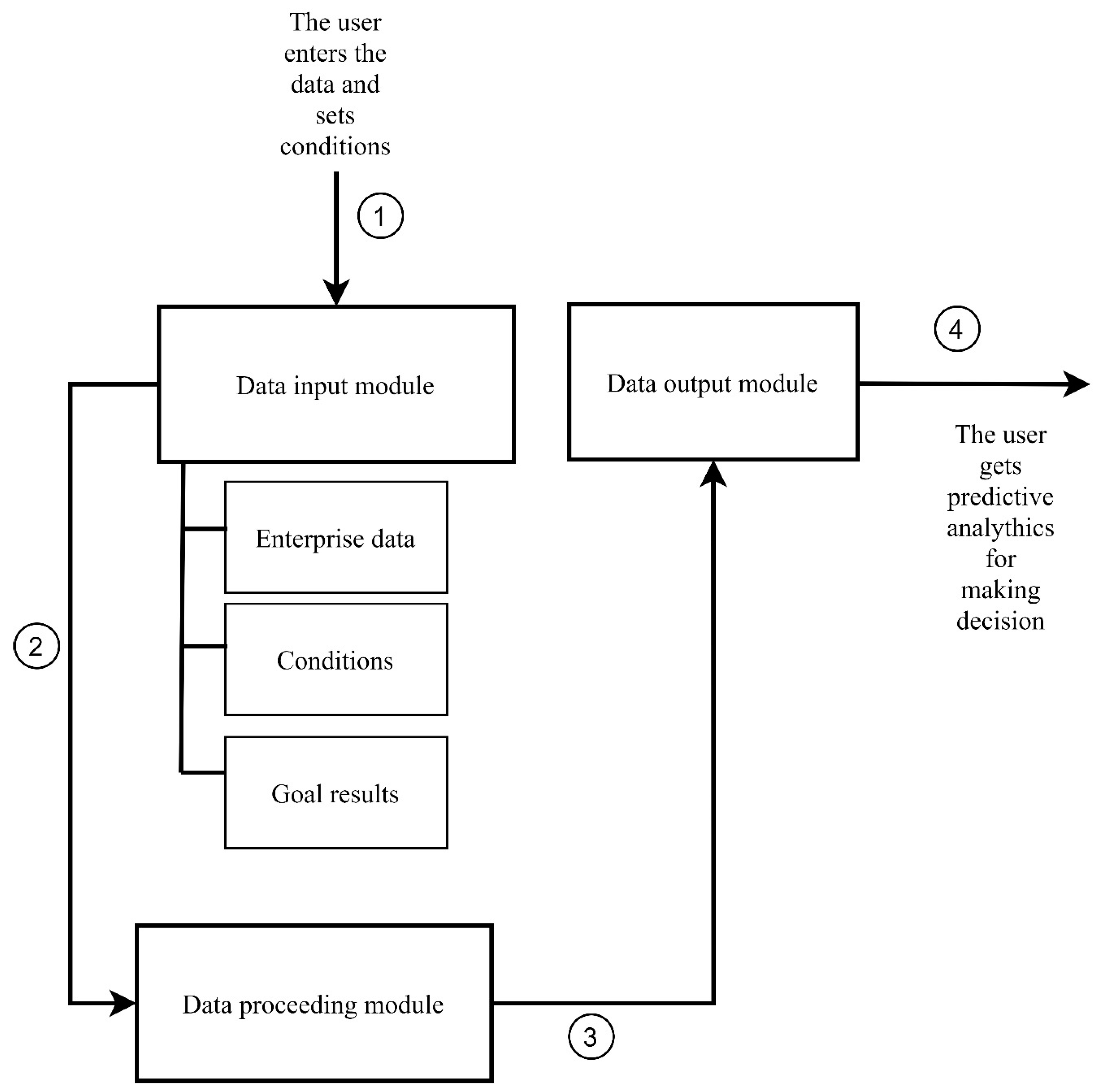
4.1. The Decision Support System for Compensation Plan Management Description

The objectives of the DSS are, firstly, to improve the efficiency of the enterprises. Secondly, to enable the DM to apply more informed decisions regarding the CS in the enterprise. Thirdly, to reduce economic risks when changing the CS at the enterprise.
In order to achieve the objectives of the DSS, it is required to solve relevant tasks, i.e., the software should have relevant functionality. This aspect is considered in the example shown in Figure 1 (software architecture developed by the authors).
As shown in Figure 1, there are 3 main modules in the DSS. The data input module allows the user to specify the quantitative options for the enterprise, as well as providing the ability to independently determine the risk level for a number of parameters and the desired output. Then, in step 2, the data processing module applies the developed statistical models for the CS. The data output module provides information for decision-making. Such information includes the predicted values of parameters at an enterprise, the probability, and the level of risk.

4.2. The Problem of Randomness and Variability CS

In the present research, two main problems in DSSs in the field of CS development are distinguished.
# 1. The factor of randomness.
The key parameters for assessing the performance of an enterprise are output—Q, product quality—G, wages—W, and workers’ satisfaction—Sat. Unfortunately, there are no statistical data from enterprises on the above parameters.
Even assuming that over a period of time t, Enterprise A collected values of indicators {Q, G, W, Sat} using CS0, before implementing CS1 and collecting the same data again, it is quite difficult to reveal a pattern of indicators changing, as multiple implementations are required. In addition, it is unproven that using CS1 instead of CS0 will give Enterprise B the same predicted result as Enterprise A. Furthermore, it is obvious to reject the notion that all of the businesses will have the same results when CS1 is used after CS0.
The reason lies in the individual and unpredictable reaction of the team and each employee to changes in the CS. The random factor applies to all parameters. For this reason, it is only possible to predict the qualitative and quantitative changes in the performance of an enterprise as a result of the implementation of the CS by relying on statistics. However, statistical data do not exist.
# 2. Variability.
Many parameters are taken into account for CSs, ranging from time tariffs to quality bonuses, as well as output bonuses and a multitude of other allowances and bonuses. The result is a high variability in the CS, multiplied by the variety of CSs, and other factors. Where the CS is the same, e.g., piece-rate CS, the enterprise charges can vary from one enterprise to another. Table 1 shows how many variants of a classic piecework-bonus CS may exist in the real economy.
Applying the distribution law to number of variables and constants: 8 × 256 = 2048 variants of piecework-bonus CSs may be studied. The calculation confirms the multivariate nature of the CS parameters and the lack of regularity in their functioning.

4.3. The Problem of the Randomness and Multivariance Nature of CS Solution

The solutions to the problems of CS variability, randomness, and uncertainty of the distribution law are clearly presented in Table 2.
The first point of Table 2 refers to decisions that rely on statistical data. There are no real statistics {Q, G, W, Sat} for the CSn at the moment. For a comparative analysis of the different types of CS and their performance, it is necessary to have data, e.g., on the monthly output of workers of different enterprises and then to compare the figures for all types of CS.
In the first case, the solution lies in the extremely problematic collection of statistical data; consequently, it is more appropriate to consider options 2 and 3 from Table 2.
The work of describing statistical models is a time-consuming but productive process. Note that, for the purposes of this paper, a statistical model of a piecework-bonus CS is considered, in which the random variables are normally distributed.

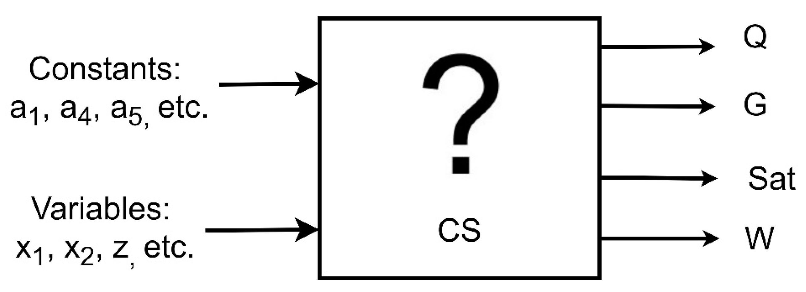
4.4. Scheme of CS Mathematical Formalization

In order to produce scientifically approved mathematical formalization, a black box model is used (see Figure 2) [42].
As shown in Figure 2, black box is a CS that transforms inputs to outputs. The black box approach states that a researcher does not know the exact method of input-to-output transformation. However, inputs and outputs are observed. In this case, the inputs are constants of the CS, which any enterprise may set, and variables, which are random for any studied company. The outputs of the black box are product output, product quality, labor satisfaction, and wage amount. So, the basic state is that values of constants and variables directly influence the results {Q, G, Sat, W} to some extent.
First conclusion: Any enterprise may see its inputs and outputs. However, the key question is what would be the results {Q, G, Sat, W} for a specific enterprise if it changes CS0 to CS4? The general answer is {Q0, G0, Sat0, W0} ≠ {Q4, G4, Sat4, W4}. As can be seen from Figure 2, the structure of the CS itself is the key. However, as noted before, the method by which inputs are transformed to outputs cannot be specified. Consequently, it may be characterized as a random process. It can be written in this way: if Q0—random output of CS0, then CS0 → CS4, Q4 = Q0 ∗ X2, where x2 is a coefficient of random changes in %. It may vary ±1–100%. The sign depends on the CS.
Second conclusion: As shown in Figure 2, the inputs have a random nature, so the outputs are also random. Moreover, as shown previously, process CS0 → CS4 is also random. Thus, the standard, well-known methodology of the theory of probability and mathematical statistics can be used for the current research. These methods are described in detail in many sources [42,43].

4.5. The Notation and Mathematical Formalization of a Piecework-Bonus CS

The following mathematical formalization is described in detail in another study [44]. To clarify, the formulas of CS are common knowledge, while the variables, constants, and their ranges are derived from an economic point of view [44]. More clarification is given in Section 4.6.
Notations:
x 1 —the output of a time-based CS, measured in c.u., is a random variable; x 1 [ 50 ; 100 ] ;
x 2 —is the effect on output during a change of CS, random variable, x 2 [ 0 ; 1 ] ;
y 1 —is the quality of output while the enterprise is running a time-based CS, in %, a random variable; y 1 [ 50 ; 100 ] ;
y 2 —impact on quality when changing CS, y 2 [ 0 ; 1 ] ;
z —workers’ satisfaction while the enterprise running a time-based CS, in %, a random variable; z [ 1 ; 100 ] ;
a 1 —is the wage while the enterprise is running a time-based CS, measured in conventional monetary units; a 1 = 10 , 000 ;
a 4 —is the tariff rate for a piecework-bonus CS, measured in conventional monetary units; a 4 [ 105 ; 117 ] ;
a 5 —is a quality bonus in a piecework-bonus CS, measured in conventional monetary units; a 5   [ 1000 ; 3000 ] ;
b 2 —is the quality standard, in %. When achieved in a piecework-bonus CS, a bonus is paid, b 2 [ 70 ; 80 ] ;
W 4 —wage fund for a piecework-bonus CS, measured in c.u;
G 4 —quality in a piecework-bonus CS, in %;
S a t 4 —workers’ satisfaction with a piecework-bonus CS, in %;
Q4—output while the enterprise is running a piecework-bonus CS, in c.u.
In the following formulas:
Q 4 = { x 1 ( 1 + x 2 )   i f   Q 4 100 100 , i f   Q 4 > 100 ,
G 4 = { y 1 ( 1 + y 2 ) , i f   y 1 b 2 b 2 , i f   y 1 > b 2 ,
W 4 = { a 4 b 2 , i f   G 4 b 2 a 4 b 2 + a 5 , i f   G 4 > b 2 ,
S a t 4 = { z + 100 ( a 4 b 2 a 1 1 ) 100 x 2 y 2 100 , i f   y 1 b 2 z + 100 ( a 4 b 2 + a 5 a 1 1 ) 100 x 2 ( b 2 y 1 1 ) 100 , i f   y 1 > b 2 ,
The range of variation of the S a t 4 value is: 1 ≤   S a t 4 100 .
Let the random variables   x 1 ,   x 2 ,   y 1 ,   y 2 ,   z be given their distribution densities f x 1 ( x 1 ) ,   f x 2 ( x 2 ) ,   f y 1 ( y 1 ) ,   f z ( z ) . The random variables x 1 ,   x 2 ,   y 1 ,   y 2 ,   z vary in the ranges:   a x 1 b , s 1 x 2 s 2 , c y 1 d , s 1 y 2 s 2 , g z h .
Here, a = 50 ,   b = 100 ; c = 50 ,   d = 100 ; g = 1 ,   h = 100 , s 1 = 0 ,   s 2 = 1 . Truncated normal distribution is used as densities f x 1 ( x 1 ) ,   f x 2 ( x 2 ) ,   f y 1 ( y 1 ) ,   f z ( z ) ; as such, the results are determined.

4.6. Model Consistency

For any model it is crucial to be adequate and reflect a real economic object. Before setting out the model’s consistency, some limitations need to be discussed. According to competent authors, any model is imperfect, because of the complexity of real objects [42,43]. Thus, modeling aims only to learn some object trends and behaviors while employing many assumptions, as discussed below.
Firstly, Section 4.5 shows that the black box model can be easily applied to CS functionality. Both inputs and outputs are described. References and common logic show that CS directly influences enterprise results such as {Q, G, Sat, W}. As such, it appears adequate to devise mathematical formalization for CS functionality.
Secondly, there are many comments about the randomness of CS functionality. Overall, the processes are influenced by the theory of probability and mathematical laws of statistics, which are well known.
Thirdly, Section 4.6. presents the units of measurement for the indicators. In essence, in the description of the statistical model, the exact units used to measure the indicators are not significant. Regardless of whether the units used are tons, megatons, m3, rubles, dollars, or billions of US dollars, the only things that matter are their functional links. This is why conventional units and conventional monetary units are used.
Fourthly, the ranges of variables and constants in Section 4.6 are derived from simple, well-known economic logic. The only thing which is important is the correlation between ranges of constants and variables. For example, the piecework tariff (a4) cannot be too low, because workers will not have the opportunity to earn its standard wage (a1). It cannot be too high either because workers will have the opportunity earn twice the wage while providing half the product output. Thus, it appears reasonable to assume that each enterprise sets a piecework tariff with a correlation to the standard time-based CS on the market.
Finally, there is the assumption of the labor satisfaction (Sat4) calculation principle. The formulas are based on the concept of «Homo economicus» proposed by A. Smith and formalized by J. S. Mill. This is a topic for a separate discussion. The general concept highlights the self-interest of the economic agent. For example, the less work an employee produces, while earning the current wage or even more, the more the employee will be satisfied with the work and vice versa. This principle is expressed in formulas.
Thus, the mathematical model of CSs may be considered as adequate, but many improvements should be made in future studies.

5. Research Results

The following results are achieved by using common methods of mathematical statistics and probability theory. All these methods are applied to formal mathematical models of CSs. Thus, the statistical model of CS results is obtained.

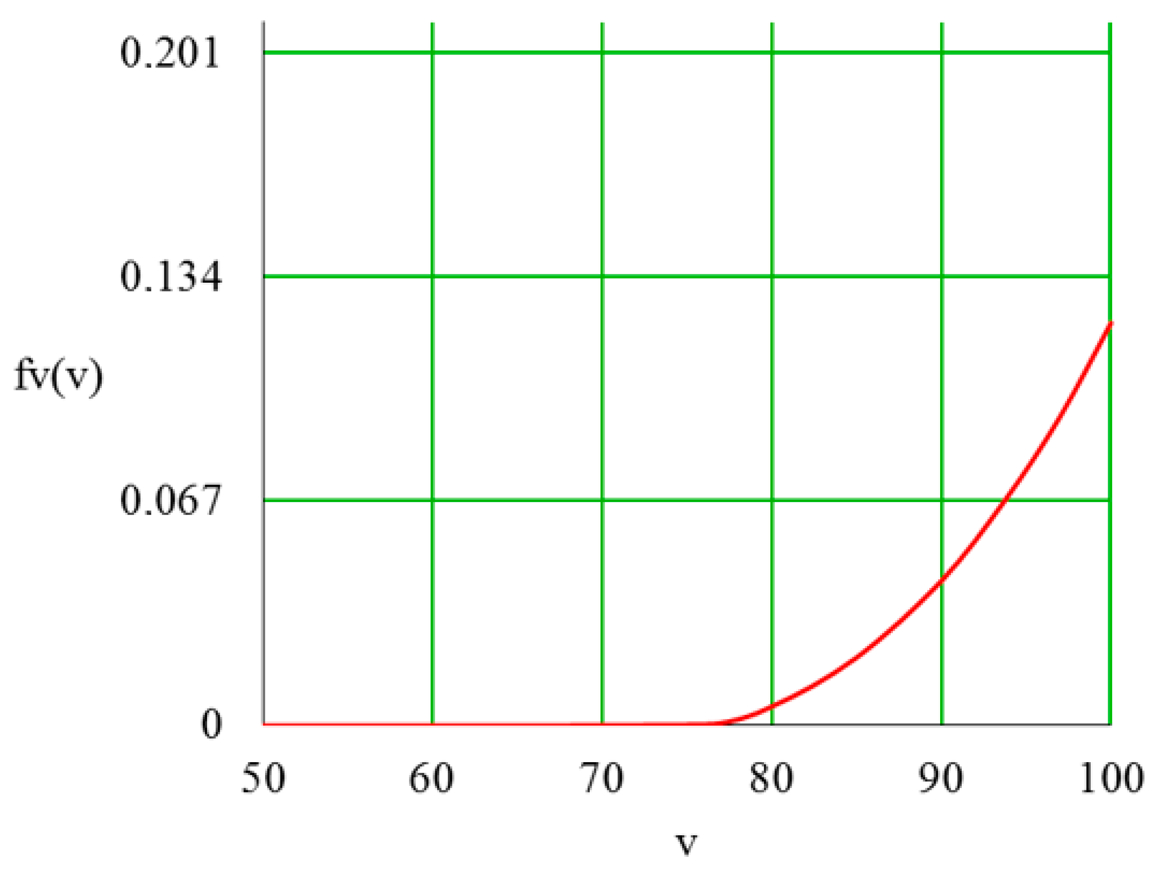
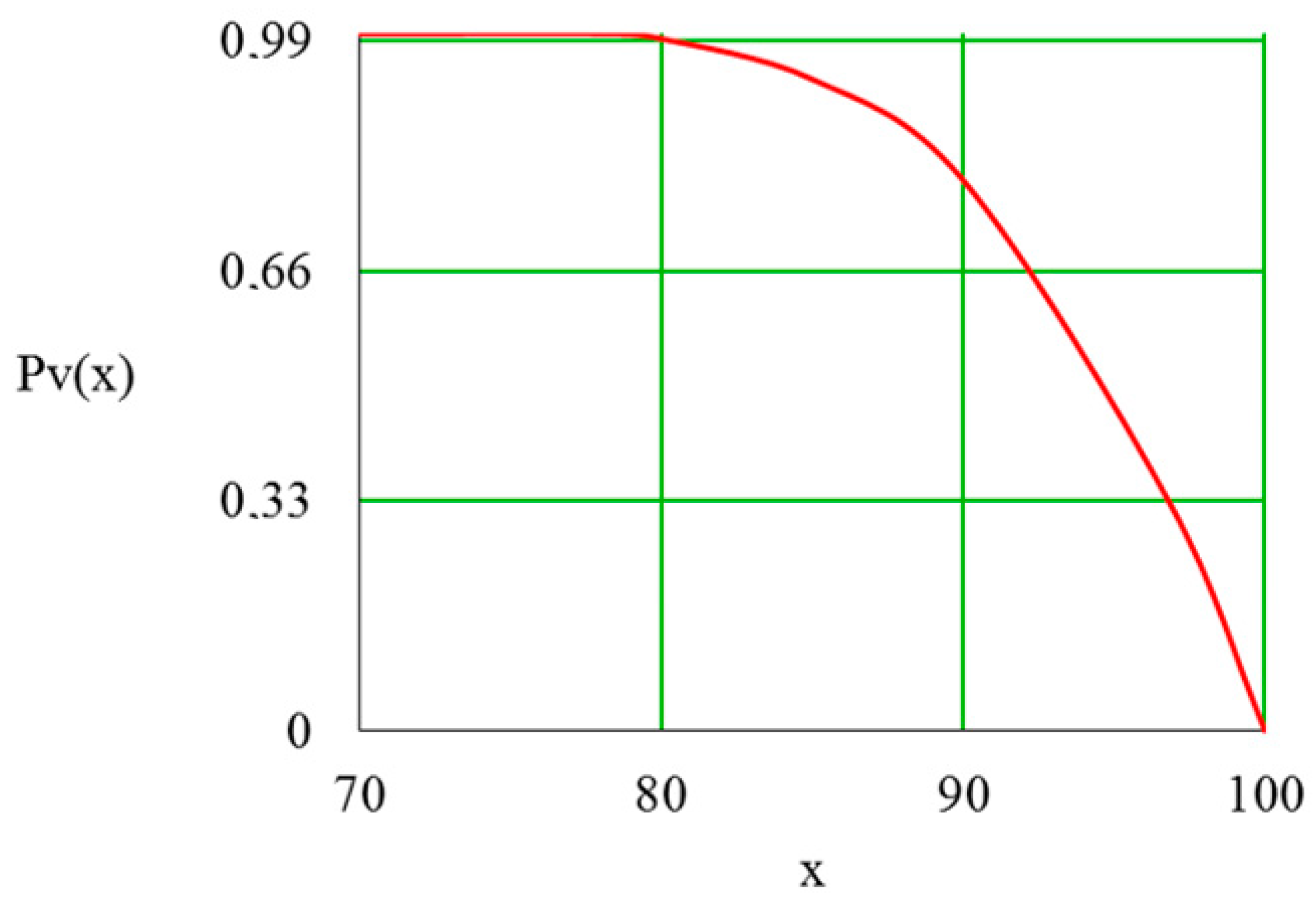
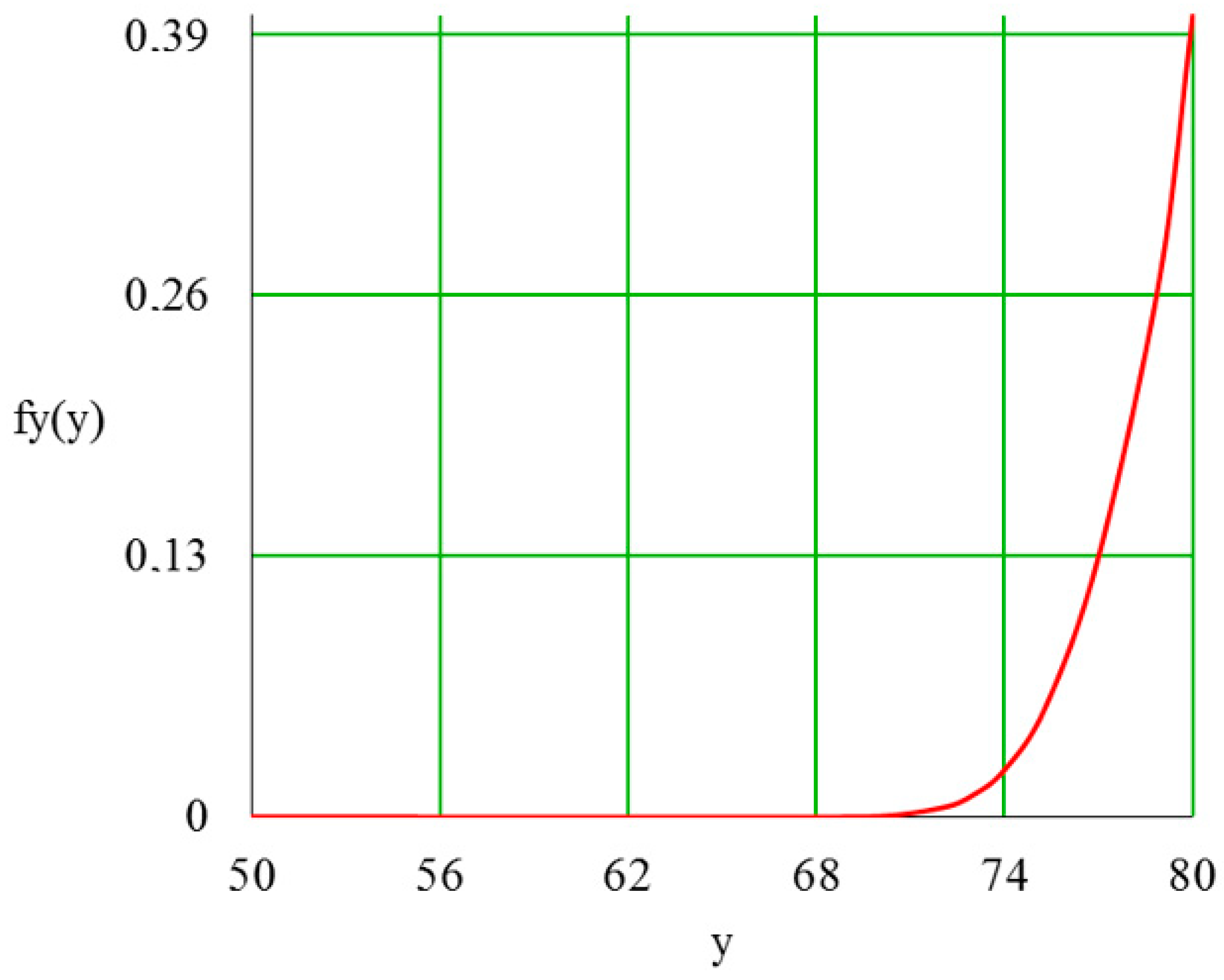
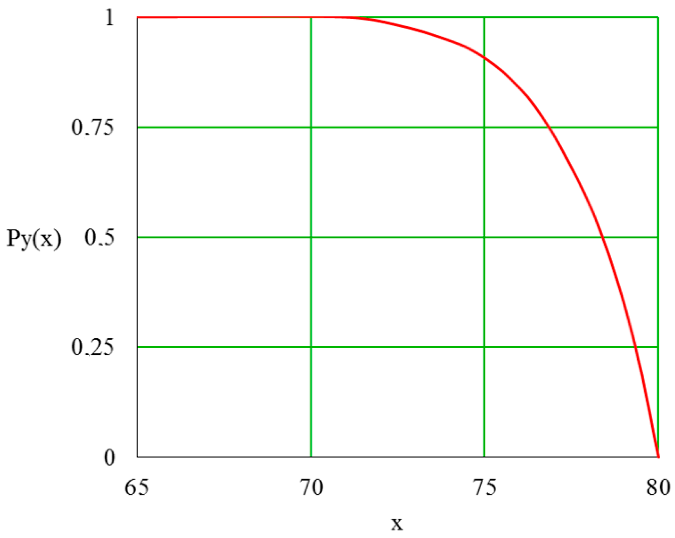
5.1. Output Distribution Density in a Piecework-Bonus CS

A random variable Q4 is considered that expresses the output of a piecework-bonus CS in a conditional unit.
Denote Q4 by v, so
v = { x 1 ( 1 + x 2 ) ,   if   v 100 100 ,   i f   v > 100 ,  
Denote q = 1 + x 2 . Probability density of q is equal to ( q ) =   f x 2 ( q 1 ) , q [ 1 ;   2 ] . Consider a random variable v = x 1 q (where Q4 = v) and find the distribution density of this value. Thus, the range of values of the variables q and v, in which the random variable v = x 1 q , is different from zero, while a q 2 = b q 1 (here q 1 = 1 ,     q 2 = 2 ). This area is presented in the form of two sub-areas: in the first sub-area, the value v changes in the range a q 1 v a q 2 ; in the second, a q 2 v b q 2 . Here, q 1 = 1 ,     q 2 = 2 .
The probability distribution of a random variable in the first sub-area is
x 1 = v q ,     d x 1 = d v q
Then, the probability density of a random variable can be calculated by the formulas:
f 1 ( v ) = q 1 v / a f q ( q ) f x 1 ( v / q ) d q q = q 1 v / a f x 2 ( q 1 ) f x 1 ( v / q ) d q q ,   a q 1 v a q 2
f 2 ( v ) = v / a q 2 f q ( q ) f 1 x 1 ( v / q ) d q q = v / a q 2 f x 2 ( q 1 ) f x 1 ( v / q ) d q q ,   a q 2 v b q 2
As output v is restricted b 1 < a q 2 = 100 , only the first sub-area has been taken into account. For the probability density of the random output variable v = Q 4 , the following expression is obtained:
f ( v ) = C v 1 v / a f x 2 ( q 1 ) f x 1 ( v / q ) d q q , a v b ,
C v = 1 a b ( 1 v / a f x 2 ( q 1 ) f x 1 ( v / q ) d q q ) d v normalization   constant ,
Example 1. Let the random variables x1 and x2 be normally distributed with parameters ( m x 1 = 85 ,   σ x 1 = 5 ; m x 2 = 0.5 ,   σ x 2 = 0.2 ). The probability density plot of the random variable v = Q4 is exposed further (Figure 3).
Characteristics of the random variable v = Q4:
v m = a b v f v ( v ) d v ,
v 2 = a b v 2 f v ( v ) d v ,  
σ v = v 2 v m 2 v m = 93.749 , σ v = 4.948
The value P v ( x ) = 1 a x f x ( x ) d x can be used as a measure of efficient labor (achieving the desired output).
The following figure shows a graph of the probability of successfully reaching a selected level of output.
Probability P ( v > X ) (Figure 4).
P v ( x ) : = 1 a x f v ( v ) d v ,
As can be seen from the graph, the probability of achieving the maximum output of 100 c.u. is close to zero. The curve also has an interesting property, namely that the probability of achieving an output between 90 and 100 c.u. decreases sharply. By contrast, between 70 and 80 c.u., the probability is close to 0.99 and starts to fall gradually between 80 and 90 c.u.
The graph demonstrates the logical behavior of workers. The piece tariff increases productivity dramatically, but not linearly. Virtually every worker is able to increase their productivity. Then, (between 80–90 c.u.) the number of teams that are able to further increase their output declines gradually. At the hardest point (90–100 c.u.), the number of workers able to maintain a high output decreases sharply. Thus, approaching the maximum output, only «star» teams remain. Therefore, the probability that the particular enterprise has such a team is close to zero.

5.2. Quality Distribution Density in Piecework-Bonus CS

At this point, consider the random variable G4 (expressing quality in a piecework-bonus CS). Denote G4 by y :
y = { y 1 ( 1 + y 2 ) ,   i f   y 1 b 2 b 2 , i f   y 1 > b 2 ,
The following expression can be derived for the density f y ( y ) :
f y ( y ) = C y q 1 y / c f y 2 ( q 1 ) f y 1 ( y / q ) d q q ,
C y = 1 c b 2 ( q 1 y / c f y 2 ( q 1 ) f y 1 ( y / q ) d q q ) d y ,
Example 2. Let random variables y 1   and y 2 be normally distributed with parameters ( m y 1 = 85 ,   σ y 1 = 5 ; m y 2 = 0.5 ,   σ y 2 = 0.2 ), Let b 2 = 80 .
The probability density plot of the random variable y = G 4   has the following form (Figure 5).
Characteristics of the random variable y = G 4
v m = c b 2 y f y ( y ) d y ,
v 2 = c b 2 y 2 f y ( y ) d y ,  
σ y = v 2 v m 2 v m = 77.783 , σ y = 1.986
P v ( x ) : = 1 c x f y ( y ) d y , graph is given in Figure 6.
Similarly, the plot of the probability of reaching the maximum quality level has a convex shape. There are also three important areas: the first is 65–70%, where the probability of achieving a selected level of quality is close to 1; the second is 70–75%, where there is a gradual decline in the probability function; the third is 75–80%, where a sharp fall in the probability is observed, down to the zero level.
However, there are two main differences from the productivity graph. Firstly, the graph in Figure 6 is flatter at 70–75%. Secondly, the quality limit is only 80%, as opposed to the output (100 c.u.). To explain these facts, it is necessary to look at how a quality bonus is given—the b2 value, which can be set from 70 to 80%. An employee receives a bonus when the b2 bar is reached. For now, it is necessary to look at each section of the graph in more detail.
Area 65–70%—the quality level that 100% of the workforce will reach, because it is not difficult to achieve and the bonus is significant. Area 70–75%—the probability that the workers will reach this quality level in exchange for the bonus is between 0.9 and 1. This is because this quality level is not too high on the one hand and the bonus is significant on the other hand. In the third area, 75–80%, function drops off sharply. This is due to the fact that 80% quality is a more difficult level to achieve; hence, few workers with the existing piecework tariff can achieve this level, and the probability will be close to zero.
The explanation for the 80% function limit is that workers have absolutely no incentive to produce higher quality products above the level for which they will get their bonuses.
Conclusion: the more your DM sets a quality bar to pay a bonus, the less likely workers will reach it. This simple thesis has economic logic and common sense and is also supported mathematically.
Calculating the characteristics of the random variable v = G 4 :
G 4 = { y 1 ( 1 + y 2 ) , i f   y 1 b 2 b 2 , i f   y 1 > b 2 ,
There are two incompatible cases—case 1 ( c y 1 b 2 ) and case 2 ( b 2 y 1 d ).
The probability of case 1 and case 2 occurrence is:
P 1 = c b 2 f y 1 ( y ) d y ,    P 2 = 1 P 1 ,
Thus, the average value of the random value v = G 4 is as follows:
m G = P 1 c b 2 y f y ( y ) d y + P 2 b 2 ,
Standard deviation:
σ G = ( c b 2 y 2 f y ( y ) d y ( c b 2 y f y ( y ) d y ) 2 ) ,
Calculation of the characteristics of the G4 variable:
P 1 = c b 2 f y 1 ( y ) d y
P 1 = 0.159 ,  
P 2 = 1 P 1 , P 2 = 0.841 ,
m G = P 1 c b 2 y f y ( y ) d y + P 2 b 2 ,  
σ G = c b 2 y 2 f y ( y ) d y ( c b 2 y f y ( y ) d y ) 2 ,
The characteristics of the calculation results of variable value v = G 4 in case 2 are as follows:
P 1 = 0.159 ;   P 2 = 0.841 ;   m G = 80 % ;   σ G = 2 % .

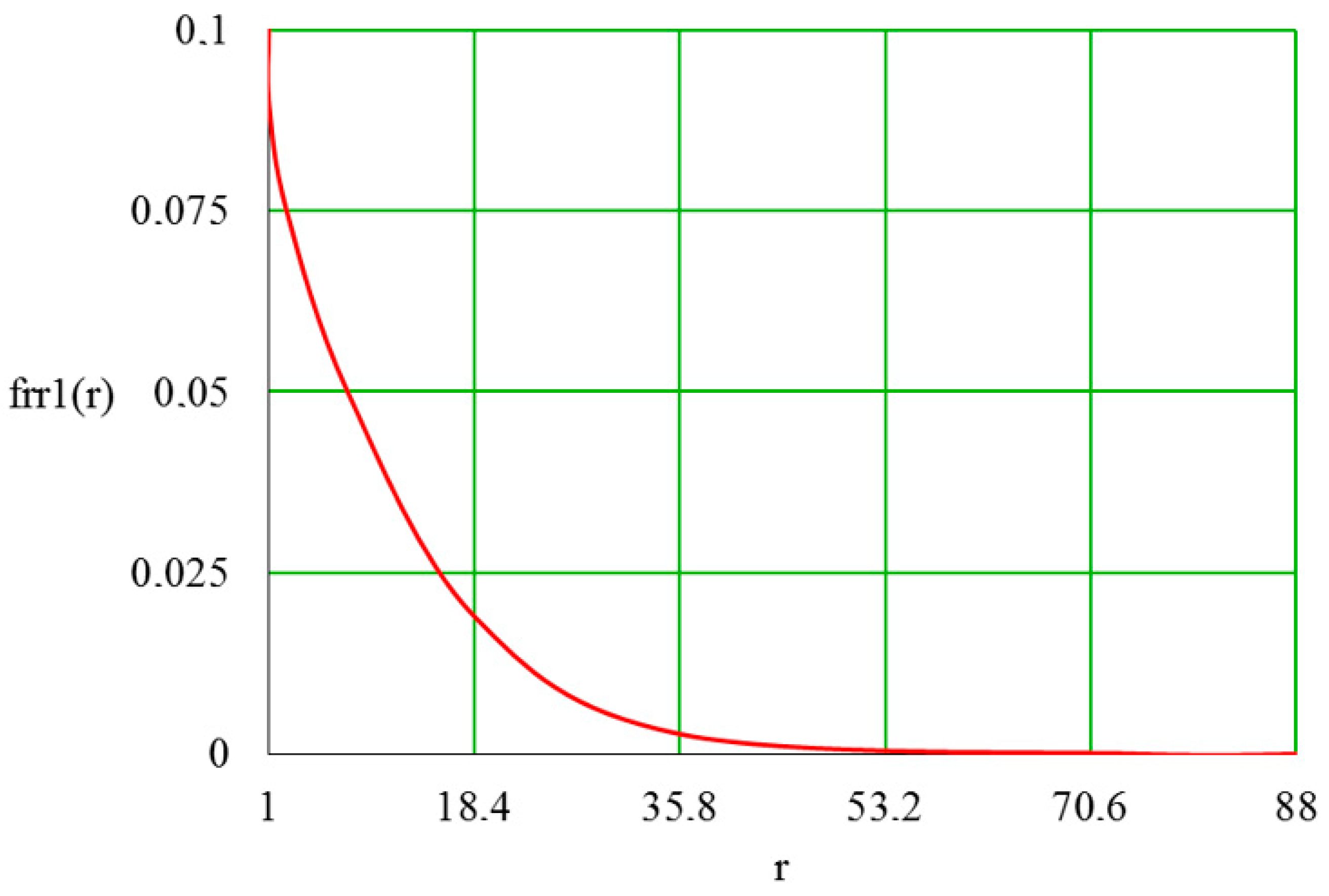
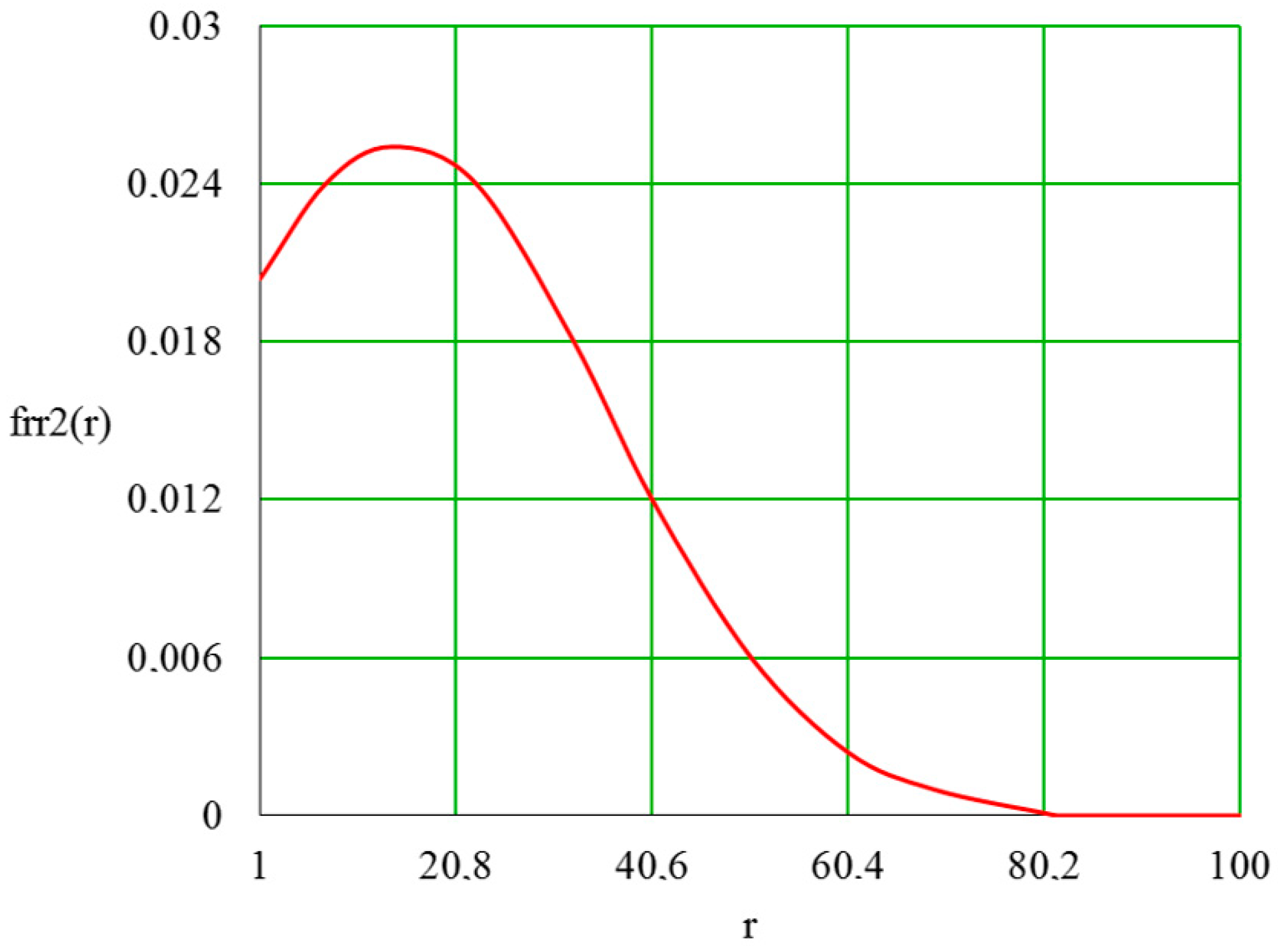
5.3. Distribution Density of a Wage Fund in a Piecework-Bonus CS

Denote the variable W 4 by.
W = { a 4 b 2   i f   G 4 b 2 a 4 b 2 + a 5 , i f   G 4 > b 2 ,
Previously, the notation y = G 4 is used and the density f y ( y ) is obtained. So, here there are two incompatible events—case 1 ( c y b 2 ) and case 2 ( b 2 y d ). To calculate the probabilities, the density f y ( y ) must be renormalized.
C y 1 = 1 c d ( q 1 y / c f y 2 ( q 1 ) f y 1 ( y / q ) d q q ) d y ,
f 1 y ( y ) = C y 1 q 1 y c f y 2 ( q 1 ) f y 1 ( y q ) d q q ,
The probability of case 1 and case 2 occurrence is:
P 1 = c b 2 f 1 y ( y ) d y ,   P 2 = 1 P 1 ,
Thus, average value of the random value W = W 4 is:
m W = P 1 ( a 4 b 2 ) + P 2 ( a 4 b 2 + a 5 ) ,
σ W = P 1 ( a 4 b 2 ) 2 + P 2 ( a 4 b 2 + a 5 ) 2 ( m W ) 2   ,  
Case 3. Let a 4 = 110 ,   a 5 = 2000 ,   and   b 2 = 80 . So, the results are follows: P 1 = 0.012 ;   P 2 = 0.988 ;   m W = 10 , 780 ;   σ W = 221 .

5.4. Distribution Density of Employee Satisfaction with Piecework-Bonus CS

Let us move on to the random value Sat4 (satisfaction with piecework-bonus CS). Denote it by   r .
Case 1: y 1 b 2 .
r = z + 100 ( a 4 b 2 a 1 1 ) 100 x 2 y 2 100 , r 1 r r 2 , s 1 x 2 s 2 ; s 1 y 2 s 2 ; h z g ; r 1 = 1 , r 2 = 100
The following notation is implemented:
M = 100 ( a 4 b 2 a 1 1 ) ; x = 100 x 2 with density f x ( x ) = f x 2 ( x / 100 ) 1 100 ; y = 100 y 2 with density f y ( y ) = f y 2 ( y / 100 ) 1 100 ; q = x + y with density
f q ( q ) = { 0 q f x ( x ) f y ( q x ) d x , 0 q 100 , q 100 100 f x ( x ) f y ( q x ) d x , 100 q 200 ,
t = M q with density f t ( t ) = f q ( M t ) ,
For the random value r = z + t for the case y 1 b 2 , probability density equals:
f r r 1 ( r ) = C r r M h f t ( r z ) f z ( z ) d z , g + M r h + M ,  
C r = 1 g h + M ( r M h f t ( r z ) f z ( z ) d z ) d r ,
The graph of random value probability density r = S a t 4 for the case y 1 b 2 is given in Figure 7.
Case 2: y 1 > b 2 .
r = z + 100 ( a 4 b 2 + a 5 a 1 1 ) 100 x 2 ( b 2 y 1 1 ) 100 ,   i f   1 > b 2 ,
r 1 r r 2 ; g z h ; s 1 x 2 s 2 ; c y 1 d ,
Observing u = ( b 2 y 1 1 ) 100 , b 2 y 1 = 100 . The density of u equals:
f u 1 ( u ) = f y 1 ( b 2 1 + u / 100 ) | b 2 ( 1 + u / 100 ) 2 | 1 100 , ( b 2 d 1 ) 100 u 0 ,
The normalization procedure is as follows:
C u = 1 b 2 d f u 1 ( u ) d u ,   f u ( u ) = C u f u 1 ( u ) ,
New notation o = x + u is applied with density
f o 1 ( o ) = { 0 o u 1 f x ( x ) f u ( o x ) d x , u 1 o 0 , o o u 1 f x ( x ) f u ( o x ) d x , 0 o 100 + u 1 o 100 f x ( x ) f u ( o x ) d x , 100 + u 1 o 100 ,
Here, u 1 = 100 ( b 2 c 1 ) , u 2 = 100 ( b 2 b 2 1 ) = 0 .
Denote M 2 = 100 ( a 4 b 2 + a 5 a 1 1 ) and implement w = M 2 o with density
f w ( w ) = f o ( M 2 w ) ,
For random value r = z + w , probability density equals:
f r r 2 ( r ) = { C r f r 1 ( r ) , g r g + w 2 ; C r f r 2 ( t ) , g + w 2 r h + w 1 C r f r 3 ( r ) , h + w 1 r h . ,
C r = 1 g g + w 2 f r 1 ( r ) d r + g + w 2 h + w 1 f r 2 ( r ) d r + h + w 1 h f r 3 ( r ) d r ,
Here
f r 1 ( r ) = g r w 1 f z ( z ) f w ( r z ) d z , g + w 1 r g + w 2 ,
f r 2 ( t ) = r w 2 r w 1 f z ( z ) f w ( r z ) d z , g + w 2 r h + w 1 ,
f r 3 ( t ) = r w 2 h f z ( z ) f w ( r z ) d z , h + w 1 r h + w 2 ,
w 1 = M 2 o 2 ,
w 2 = M 2 o 1 ,
The random value r = S a t 4 for case y 1 > b 2 ; the probability density graph is presented in Figure 8.
The characteristics of a random variable r = S a t 4 are calculated:
r = { z + 100 ( a 4 b 2 a 1 1 ) 100 x 2 y 2 100 , i f   y 1 b 2 z + 100 ( a 4 b 2 + a 5 a 1 1 ) 100 x 2 ( b 2 y 1 1 ) 100 , i f   y 1 > b 2 ,
There are two incompatible cases. Case 1 ( c y 1 b 2 ) and case 2 ( b 2 y 1 d ). The realization probability of case 1 and case 2 is:
P 1 = c b 2 f y 1 ( y ) d y ,
P 2 = 1 P 1 ,
Thus, the average value of the random value r = S a t 4 equals
m S = P 1 g h r f r r 1 ( r ) d r + P 2 g h r f r r 2 ( r ) d r
Random value standard deviation calculation r = S a t 4 :
S 2 = P 1 g h r 2 f r r 1 ( r ) d r + P 2 g h r 2 f r r 2 ( r ) d r ,
σ S = S 2 m S 2 ,
The characteristics (mean value, standard deviation) of variable S a t 4 (satisfaction with piecework-bonus CS) are calculated as follows:
P 1 = c b 2 f y 1 ( y ) d y , P 1 = 0.159
P 2 = 1 P 1 , P 2 = 0.841
m S = P 1 g h r f r r 1 ( r ) d r + P 2 g h r f r r 2 ( r ) d r ,
S 2 = P 1 g h r 2 f r r 1 ( r ) d r + P 2 g h r 2 f r r 2 ( r ) d r ,
σ S = S 2 m S 2
Case 4. Let a4 = 110, a5 = 2000, and b2 = 80. The results are: P 1 = 0.159 ; P 2 = 0.841 ; m S = 22 % ;   σ S = 15 % .

5.5. Applying a Statistical Model to the Data Processing Module of the DSS

The resulting probability densities are effectively used in the data processing module (Figure 1). The following algorithm is used:
  • The user specifies which indicator values they would like to obtain {Q, G, Sat, W};
  • The user sets (in %) the level of risk they are prepared to accept in case MD in relation to the CS fail;
  • The software processing module calculates statistical characteristics of CS parameters;
  • The result for the MD is shown.
For example, if the user wants to change from a time-tariff to a piecework-bonus CS, the user should achieve an output value   Q 4 (the output of a piecework-bonus CS) of at least 95 c.u. According to the derived probability density, the probability of this event will be:
P ( Q 4 95 ) = 1 50 95 f ( Q 4 ) d Q 4 = 17.3 % ,
Thus, the information for MD is presented. Whether a manager is willing to change the CS to obtain a high output result has a probability of 17%.
Other indicators are calculated in a similar way. For example, when a user wants to achieve a quality level of at least 75%, the probability of this happening would be 0.9.
Nevertheless, the data processing module of the DSS is more complex, partly because it operates several statistical models for different CSs. In the end, MD are reduced to the user making a weighted choice between the desired indicators and the probability of their realization.

6. Conclusions

The purpose of this paper was to develop a statistical model of a piecework-bonus CS, to be used in the data processing module of the CS DSS. Existing CS models do not take into account the random behavior of CS indicators, which means that the models are of little use. In order to build practically useful models, it is necessary to have statistical data, which are not available at present. This paper proposes two main approaches to solve the problem: (1) creating algorithmic statistical CS models and (2) developing CS simulation models. This paper presents a statistical model of a piecework-bonus CS obtained under the assumption of a normal distribution of initial values. The formulas for the probability densities of the resulting indicators of the piecework-bonus CS were obtained, so the statistical characteristics of CS indicators were calculated, as were the probabilities of achieving the desired results. The main conclusions are as follows:
  • It is possible to obtain and effectively apply algorithmic statistical models of CS in the CS DSS module.
  • Analytical statistical models for CS are possible to obtain only with an even distribution of the initial CS data. However, even for this simple case, the resulting CS model seems to be more practical than the deterministic CS models.
  • As a limitation, it must be mentioned that for more complex probability distributions of initial data (normal distribution, chi-square distribution, and others), the formulas for the probability densities of the resulting CS indicators become too complex and difficult to interpret.
  • Further development of CS models is possible based on simulation modeling. The simulation modeling method allows the modeling of any process influenced by random factors. It is also a universal method for solving mathematical tasks.
  • There is potential for further CS research using a statistical models method. This includes defining the most significant distribution laws of CS model variables and then applying them to the presented algorithmic statistical model. These extensive results may be of great use in building DSSs and studying CSs.

Author Contributions

Conceptualization, A.M., A.S. (Aleksandr Shilnikov), P.S. and A.S. (Anatoly Sidorov); review of sources, A.M., A.S. (Aleksandr Shilnikov) and P.S.; description of the method, A.M. and A.S. (Aleksandr Shilnikov); experiment (testing, calculations), A.S.; writing—original draft preparation, A.M. and A.S. (Aleksandr Shilnikov); writing—review and editing, P.S.; visualization, A.M. and A.S. (Aleksandr Shilnikov); funding acquisition, P.S. All authors have read and agreed to the published version of the manuscript.

Funding

This research was funded by Ministry of Science and Higher Education of the Russian Federation; project FEWM-2020–0036.

Institutional Review Board Statement

Not applicable.

Informed Consent Statement

Not applicable.

Data Availability Statement

Not applicable.

Conflicts of Interest

The authors declare no conflict of interest.

References

  1. Yabanci, O. From human resource management to intelligent human resource management: A conceptual perspective. Hum.-Intell. Syst. Integr. 2019, 1, 101–109. [Google Scholar] [CrossRef]
  2. Kraev, V.; Tikhonov, A. Risk Management in Human Resource Management. TEM J. 2019, 8, 1185–1190. [Google Scholar] [CrossRef]
  3. Turker, D. Social Responsibility and Human Resource Management. In Managing Social Responsibility. CSR, Sustainability, Ethics & Governance; Springer: Cham, Switzerland, 2018; pp. 131–144. [Google Scholar]
  4. Brink, W.; Kuang, X.; Majerczyk, M. The effects of minimum-wage increases on wage offers, wage premiums and employee effort under incomplete contracts. Account. Organ. Soc. 2021, 89, 101195. [Google Scholar] [CrossRef]
  5. Rajibul, A.M.; Kijima, Y. Can a Higher Wage Attract Better Quality Applicants without Deteriorating Public Service Motivation? Evidence from the Bangladesh Civil Service. Int. J. Public Adm. 2021, 44, 74–89. [Google Scholar] [CrossRef] [Green Version]
  6. Habel, J.; Alavi, S.; Linsenmayer, K. Variable Compensation and Salesperson Health. J. Mark. 2021, 85, 130–149. [Google Scholar] [CrossRef]
  7. Chung, C.; Sung Hoon, K.; Koangsung, C. Effects of wage-peak system on youth employment: Evidence from South Korea. Appl. Econ. 2021, 53, 4975–4984. [Google Scholar] [CrossRef]
  8. Morris, M.; Chen, H.; Heslin, M.J.; Krontiras, H. A Structured Compensation Plan Improves But Does Not Erase the Sex Pay Gap in Surgery. Ann. Surg. 2018, 268, 442–448. [Google Scholar] [CrossRef] [PubMed]
  9. Deelen, A. Flexible Wages or Flexible Workers? A Decomposition of Wage Bill Adjustment by Dutch Firms, 2006–2013. Economist 2021, 169, 179–209. [Google Scholar] [CrossRef]
  10. Bechter, B.; Braakmann, N.; Brandl, B. Variable Pay Systems and/or Collective Wage Bargaining? Complements or Substitutes? ILR Rev. 2021, 74, 443–469. [Google Scholar] [CrossRef] [Green Version]
  11. Yang, R.; Mai, Y.; Lee, C.-Y.; Teo, C.-P. Tractable Compensation Plan under Asymmetric Information. Prod. Oper. Manag. 2020, 29, 1212–1218. [Google Scholar] [CrossRef]
  12. Edmans, A.; Gabaix, X. Executive Compensation: A Modern Primer. J. Econ. Lit. 2016, 54, 1232–1287. [Google Scholar] [CrossRef] [Green Version]
  13. Zhou, B.; Li, Y.-M.; Sun, F.-C.; Zhou, Z.-G. Executive compensation incentives, risk level and corporate innovation. Emerg. Mark. Rev. 2021, 47, 100798. [Google Scholar] [CrossRef]
  14. Chung, K.; Boutaba, R.; Hariri, S. Knowledge based decision support system. Inf. Technol. Manag. 2016, 17, 1–3. [Google Scholar] [CrossRef] [Green Version]
  15. Jason, L.; Sukari, F.; Geoffrey, B. Biased self-assessments, feedback, and employees’ compensation plan choices. Account. Organ. Soc. 2016, 54, 45–59. [Google Scholar] [CrossRef]
  16. Pylkkänen, E. Modeling Wages and Hours of Work. In Proceedings of the 6th Nordic Seminar On Micro Simulation Models, Copenhagen, Denmark, 8–9 June 2000; pp. 1–47. [Google Scholar]
  17. Orlova, E. Innovation in Company Labor Productivity Management: Data Science Methods Application. Appl. Syst. Innov. 2021, 4, 68. [Google Scholar] [CrossRef]
  18. Bolgova, E.V. Modeling the behavior of the wage fund at various levels of staffing of the enterprise. Bull. Samara State Acad. Railw. 2014, 6, 60–64. [Google Scholar]
  19. Joseph, G.; Altonji, A.; Smith, A. Modeling earnings dynamics. Econometrica 2013, 81, 1395–1454. [Google Scholar] [CrossRef]
  20. Lupinos, E.A. Modeling the wage system. Omsk. Univ. Bull. Ser. Econ. 2011, 1, 122–126. [Google Scholar]
  21. Kustandi, C.; Reni, A.; Suharto, T.; Lestari, N. Providing Best Employee Rewards using Decision Support System Method. Int. J. Adv. Sci. Technol. 2020, 29, 6356–6363. [Google Scholar]
  22. Setiawan, N.; Rossanty, Y. Simple Additive Weighting as Decision Support System for Determining Employees Salary. Int. J. Eng. Technol. 2018, 7, 309–313. [Google Scholar]
  23. Irawan, Y. Decision Support System for Employee Bonus Determination with Web-Based Simple Additive Weighting (SAW). J. Appl. Eng. Technol. Sci. (JAETS) 2020, 2, 7–13. [Google Scholar] [CrossRef]
  24. Orlov, A.I. The development and approvement management decisions. Sci. J. KubSAU 2017, 130, 567–597. [Google Scholar]
  25. Vinogradova, E.Y. Topical issues of design and implementation of corporate management decision-making support systems at an enterprise. News Far East. Fed. Univ. Econ. Manag. 2018, 1, 102–111. [Google Scholar] [CrossRef]
  26. Bobrovnikova, A. Razvitie form i sistem oplaty truda v usloviyah rynochnoj ekonomiki Rossii. Territ. Nauk. 2017, 2, 175–178. (In Russian) [Google Scholar]
  27. Kochelorova, G. Sovershenstvovanie poryadka oplaty truda na predpriyatii. Soc.’no-Ekonomicheskij Gumanit. Zhurnal Krasnoyarskogo GAU 2018, 1, 28–41. (In Russian) [Google Scholar]
  28. Sokolova, A.; Duborkina, I. Sistema oplaty truda v kommercheskih organizaciyah. Serv. Ross. Rubezhom 2017, 11, 111–121. (In Russian) [Google Scholar]
  29. Filippova, T.; Zhabunin, A.; Ekova, V.; Shipunova, I. Ways to improve wages at the enterprise. Innov. Econ. Prospect. Dev. Improv. 2017, 1, 171–175. (In Russian) [Google Scholar]
  30. Slepcova, E.; Knyazeva, A. Optimization of wages in modern conditions. Econ. Bus. 2017, 1, 95–98. (In Russian) [Google Scholar]
  31. Borzhesh, A.; Lebedev, A. Methodological approach to assessing the effectiveness of management decision support systems in oil and gas corporations. Belgorod State Univ. Sci. Bull. 2018, 45, 239–250. [Google Scholar]
  32. Kitsios, F.; Kamariotou, M. Decision Support Systems and Business Strategy: A conceptual framework for Strategic Information Systems Planning. In Proceedings of the 6th IEEE International Conference on IT Convergence and Security (ICITCS2016), Prague, Czech Republic, 26 September 2016; pp. 149–153. [Google Scholar]
  33. Kaklauskas, A. Intelligent Decision Support Systems. In Biometric and Intelligent Decision Making Support; Springer: Cham, Switzerland, 2015; pp. 31–85. [Google Scholar]
  34. Demidovskij, A.; Babkin, E. Developing a distributed linguistic decision making system. Bus. Inform. 2019, 13, 18–32. [Google Scholar] [CrossRef] [Green Version]
  35. Aqell, M.; Nakshabandi, O.; Adeniyi, A. Decision Support Systems Classification in Industry. Period. Eng. Nat. Sci. 2019, 7, 774–785. [Google Scholar] [CrossRef] [Green Version]
  36. Rashidi, M.; Ghodrat, M.; Samali, B.; Mohammadi, M. Decision Support Systems. Manag. Inf. Syst. 2018, 2, 19–38. [Google Scholar]
  37. Sidorov, A.; Senchenko, P. Regional Digital Economy: Assessment of Development Levels. Mathematics 2020, 8, 2143. [Google Scholar] [CrossRef]
  38. Vinogradova, E. Questions of design corporate systems for support of acceptance of administrative decisions at the enterprise. Bull. Far East. Fed. Univ. Econ. Manag. 2018, 1, 102–111. [Google Scholar] [CrossRef]
  39. Karamyshev, A. Process-based management methodology analysis completely covering business processes of the enterprise. Bull. Belgorod State Technol. Univ. Named After. V. G. Shukhov 2017, 2, 214–217. [Google Scholar] [CrossRef]
  40. Osipov, V.; Gorina, A. Characteristic and directions of development of management accounting systems. [Harakteristika i napravleniya razvitiya sistem upravlencheskogo ucheta]. Vestn. Univ. 2019, 5, 40–47. [Google Scholar] [CrossRef]
  41. Shvedenko, V. Information support of interaction of process and functional management of enterprise activities. Izv. St.-Peterbg. Gos. Ekon. Univ. 2019, 6, 90–94. [Google Scholar]
  42. Borovkov, A.A. Applied Statistics; University Textbook; Lani: Saint-Petersburg, Russia, 2021; 704p. [Google Scholar]
  43. Davison, A.C. Statistical Models; Cambridge University Press: Cambridge, UK, 2008; 726p. [Google Scholar]
  44. Shilnikov, A.; Mitsel, A. Management of the compensation system based on statistical models and simulation. Vestn. Astrah. Gos. Tekhnicheskogo Univ. 2021, 3, 82–93. [Google Scholar]
Figure 1. Description of the DSS modules.
Mathematics 09 03126 g001
Figure 2. Black box model.
Mathematics 09 03126 g002
Figure 3. The probability density plot—Q4.
Mathematics 09 03126 g003
Figure 4. The probability of successfully reaching a set level of output.
Mathematics 09 03126 g004
Figure 5. The probability density plot—G4.
Mathematics 09 03126 g005
Figure 6. The probability of successfully reaching a set level of quality.
Mathematics 09 03126 g006
Figure 7. The labor satisfaction (Sat4) probability density ( y 1 b 2 ) .
Mathematics 09 03126 g007
Figure 8. The labor satisfaction (Sat4) probability density ( y 1 > b 2 ).
Mathematics 09 03126 g008
Table 1. Piecework-bonus CS variability.
ParameterValueQuantity
CSPiecework bonus1 CS
Variables and constantsAccording to mathematical formalization (see Section 4.5). Value of each variable and constant varies in its own range.8 units
The distribution lawThe values of variables and constants in the CS differ according to the enterprise. So, for researchers these are random. It is not possible to choose a distribution law; it is necessary to select from a number of known laws. As an example, 4 laws: even, lognormal, chi-square, and normal will be applied.4 Laws of distribution = 256 combinations
Table 2. Comparison of solutions to CS variability problems.
#The SolutionThe Essence
1Based on statistical dataProbabilistic forecasts are based on statistics. Statistical data on the types and results of CSs in different enterprises are required.
2Based on statistical modelsBased on the analysis of statistical models, the probability density of a particular CS outcome is calculated.
3Based on simulation modelingBased on the CS simulation model, generated indicators are derived to be investigated and analyzed.
Publisher’s Note: MDPI stays neutral with regard to jurisdictional claims in published maps and institutional affiliations.

