Continuous Stability TS Fuzzy Systems Novel Frame Controlled by a Discrete Approach and Based on SOS Methodology

Abstract

Generally, the continuous and discrete TS fuzzy systems’ control is studied independently. Unlike the discrete systems, stability results for the continuous systems suffer from conservatism because it is still quite difficult to apply non-quadratic Lyapunov functions, something which is much easier for the discrete systems. In this paper and in order to obtain new results for the continuous case, we proposed to connect the continuous with the discrete cases and then check the stability of the continuous TS fuzzy systems by means of the discrete design approach. To this end, a novel frame was proposed using the sum of square approach (SOS) to check the stability of the continuous Takagi Sugeno (TS) fuzzy models based on the discrete controller. Indeed, the control of the continuous TS fuzzy models is ensured by the discrete gains obtained from the Euler discrete form and based on the non-quadratic Lyapunov function. The simulation examples applied for various models, by modifying the order of the Euler discrete fuzzy system, are presented to show the effectiveness of the proposed methodology.

1. Introduction

Since their introduction in 1985, Takagi Sugeno fuzzy models have been studied for the control of a wide class of nonlinear systems owing to their ability to deal with complex behaviors [1]. In this case, the nonlinear systems can be represented by a set of linear subsystems linked to nonlinear functions. Based on the Parallel Distributed Compensation (PDC) controller and the Lyapunov function, the closed loop stability is verified leading to a Linear Matrix Inequality (LMI) that can be solved to obtain the controller gains. The LMI conditions suffer from conservatism. Therefore, to relax the LMI conditions of stability and stabilization using the candidate Lyapunov functions, many stability studies have been carried out for the continuous and discrete systems [2,3,4,5,6,7]. Since it is difficult to use the non-quadratic Lyapunov functions for the continuous systems, this type of functions can be used in the discrete case leading to LMI problems that can be solved easily. For the continuous systems, a similar approach allows for producing Bilinear Matrix Inequality (BMI) conditions that are difficult to resolve. In the work of References [8,9,10,11,12], a relaxed scheme for controller synthesis of continuous-time systems in the Takagi-Sugeno form, based on non-quadratic Lyapunov functions and a non-PDC control law, is presented, which is proved to reduce conservativeness compared with common Lyapunov functions. The obtained results suffer from conservatism. In fact, the provided relaxations allow state and input dependence of the membership functions’ derivatives, as well as independence on initial conditions when input constraints are needed. It is true that nonquadratic Lyapunov functions may be used with continuous approaches, but either they assume hypothesis about the derivative of the membership functions that must be checked a posteriori during experiments or simulations, or they are very complex, or they provide only local results [8,9,10,11,12]. Since it is not possible to enforce such constraints in the control law through LMIs, the validity of such approaches can be questioned. Indeed, a valid simulation does not imply the same validity for other initial conditions.

Several research studies tried to fuse continuous and discrete systems based on the discrete controller [13,14]. In Reference [15], the authors studied a particular class of continuous fuzzy models, i.e., the ones that can be exactly discretized. Of course, this is a restricted class, but, for this class, the continuous model behaves exactly as the discretized one. Through examples, continuous control laws may be outperformed in some cases by means of discrete control laws, including the regulator problem. In addition, the authors of Reference [16] proposed an idea for the continuous stability system by merging the two cases in order to reach new continuous results. Contrary to Reference [15], they attempted to deal with all continuous models and defined their discretized forms based on the Euler approximation method limited to the first order.

This led to two sets of LMIs conditions: one for the discrete case in order to determine the discrete control laws obtained from the Euler discretized model, and the other for the continuous case when checking the continuous stabilization systems based on the obtained discrete controller. This proposed solution led to use non-quadratic Lyapunov functions in the continuous case to avoid BMI since some parameters of the discrete control law were saved. Based on the last controller, the LMI stability conditions of the continuous models were checked using a candidate Lyapunov function. Several attempts have been made, in this context, using a quadratic and non-quadratic Lyapunov function but no solution is found by solving the LMI conditions. In Reference [16], the authors used the quadratic Lyapunov function that does not guarantee the feasibility of the solutions at all times. The last result may be explained by the choice of the Lyapunov function since the quadratic Lyapunov function cannot check the stability of the continuous model via the discrete gains obtained from its Euler discretized model, which is restricted to one. Therefore, it is important to choose the right Lyapunov function so as to achieve interesting results.

While some studies focused on the LMI conditions, another trend studied the stability analysis of polynomial fuzzy models based on the sum of squares techniques (SOS). In this case, convex optimization problems as LMI conditions are reformulated as sum of square decomposition problems [17,18,19,20,21,22,23,24]. This approach was intended for modeling and controlling nonlinear systems using polynomial fuzzy models.

Based on the polynomials’ techniques, the originality of this research work is to check the continuous stability model, controlled by the discrete gains obtained from its Euler discretized model, using the sum of squares approach. In this context, the second set of LMIs is replaced by the candidate Lyapunov polynomial function in order to show the stability of the TS continuous closed loop based on the obtained discrete controller.

Contrarily to References [15,16], in our present paper, we tried to work for all types of fuzzy continuous models, which is an advantage, and defined their discretized fuzzy models using the Euler discretization method for an order of approximation greater than one to determine the controller gains. Moreover, the stability conditions of the sum of squares do not require the derivative hypothesis of the membership functions. In addition, they guarantee the global asymptotical stability when a solution to the SOS-based optimization problem holds. Therefore, one of the advantages of our methodology is that the drawbacks of LMI conditions based on non-quadratic approaches would be overcome.

The remaining of this paper is structured as follows. Section 2 presents the materials and methods. First, the literature on the Takagi Sugeno continuous fuzzy models is reviewed. Second, the sum of squares approach (SOS) with its stability conditions based on the polynomial Lyapunov function is introduced. Then, the proposed methodology based on the Euler discretization method and SOS approach is described. Section 4 provides the illustrations of two numerical examples to prove the effectiveness of this method and exposes the simulation results and the discussions.

2. Materials and Methods

2.1. Takagi Sugeno Continuous Systems

2.1.1. Notations

Considering function $h_i\left(z(\cdot )\right)\ge 0$, and matrice $Y_i$ with $i\in \left\{1,\dots ,r\right\}$, we suggest these notations:

• $Y_z={\displaystyle \sum _{i=1}^r{h}_i\left(z\left(t\right)\right)}{Y}_i, \mathrm{in} \mathrm{the} \mathrm{discrete} \mathrm{case} Y_z={\displaystyle \sum _{i=1}^r{h}_i\left(z\left(k\right)\right)}{Y}_i$
• $\begin{array}{l}{Y}_{z+}={\displaystyle \sum _{i=1}^r{h}_i\left(z\left(k+1\right)\right)}{Y}_i,\\ Y_{zz+}={\displaystyle \sum _{i=1}^r{\displaystyle \sum _{j=1}^r{h}_i}\left(z\left(k\right)\right)h_j\left(z\left(k+1\right)\right)}{Y}_{ij},\\ Y_z^{-1}={\left({\displaystyle \sum _{i=1}^r{h}_i\left(z\left(k\right)\right)Y_i}\right)}^{-1},\hspace{0.17em}\\ Y\in \left\{A,B,K,G,P\right\}\end{array}$.

The $(*)$ indicates a transpose quantity. For example, $Y_z^T{P}_z(*)-P_z<0$ stands for $Y_z^T{P}_z{Y}_z-P_z<0$, and $\left[\begin{array}{cc}-P_z^{}& (*)\\ Y_z& -P_z^{}\end{array}\right]<0$ for $\left[\begin{array}{cc}-P_z^{}& Y_z^T\\ Y_z& -P_z^{}\end{array}\right]<0$.

Based on these forms, a TS continuous is presented as follows [1]:

$$\dot{x}\left(t\right)=A_{cz\left(t\right)}^{}x\left(t\right)+B_{cz\left(t\right)}^{}u\left(t\right).$$

(1)

The index $c$ designates the continuous case, $x\left(t\right)\in R^n$ is the vector of states, $z\left(t\right)$ is the vector of premises, $u\left(t\right)\in R^m$ is the vector of inputs, $r$ is the number of rules, and $A_{cz(t)}^{}$ and $B_{cz(t)}^{}$ are the continuous matrices of appropriate dimensions. The weights $h_i$ satisfy the following convex sum:

$${\displaystyle \sum _{i=1}^r{h}_i\left(z\left(t\right)\right)=1}.$$

(2)

2.1.2. Quadratic Stabilization Conditions

This paragraph aims to remind the reader of some results obtained by applying the Takagi Sugeno continuous model using the classical PDC law [25]. The last is defined in Equation (3):

$$u\left(t\right)=-F_{cz\left(t\right)}^{}x\left(t\right).$$

(3)

Based on Equation (3), the Takagi-Sugeno continuous fuzzy system is as follows:

$$\dot{x}\left(t\right)=\left(A_{cz\left(t\right)}^{}-B_{cz\left(t\right)}^{}{F}_{cz\left(t\right)}^{}\right)x\left(t\right).$$

(4)

The synthesis of the controller (3) allows finding the gains $F_{ci}^{}$, which ensures the continuous fuzzy system closed loop stabilization (4). The quadratic Lyapunov function is mainly used:

$$V\left(x\left(t\right)\right)=x^T\left(t\right)Px\left(t\right),\hspace{0.17em}P=P^T>0.$$

(5)

Theorem 1

([2]). The equilibrium of the system (4) is globally asymptotically stable if a common matrix $X=X^T>0$ and matrices $M_i$ satisfy these LMIs:

$$\{\begin{array}{ll}{\mathrm{Y}}_{ii}<0& i=1,2,\dots ,r\\ \frac{2}{r-1}{\mathrm{Y}}_{ii}+{\mathrm{Y}}_{ij}+{\mathrm{Y}}_{ji}<0& i,j=1,2,\dots ,r,\hspace{1em}i\ne j\end{array},$$

(6)

with: ${\mathrm{Y}}_{ij}=A_{ci}^{}X-B_{ci}^{}{M}_j+(*),\hspace{0.17em}\hspace{0.17em}X=P^{-1},\hspace{0.17em}\hspace{0.17em}{F}_{ci}^{}=M_i^{-1}X$.

2.2. Continuous Stability Conditions from the Sum of Square Approach

2.2.1. Definition

A scalar polynomial is $g\left(x\left(t\right)\right)$, a sum of squares if there are polynomials $g_i\left(x\left(t\right)\right)\hspace{0.17em}\hspace{0.17em}\forall \hspace{0.17em}i\in \left\{1,\dots ,v\right\}$ and $x\in R^n$ such that [17]:

$$f\left(x\left(t\right)\right)={\displaystyle \sum _{i=1}^v{g}_i^2\left(x\left(t\right)\right)}.$$

(7)

If $g\left(x\left(t\right)\right)$ is a sum of squares, it implies that $g\left(x\left(t\right)\right)$. Thus, this last condition will be replaced by $g\left(x\left(t\right)\right)$ as a sum of squares that can be rewritten as a convex problem. In this case, the standard solvers for LMIs can be used. The free toolbox of MATLAB, called SOSTOOLS, aims to translate these conditions into LMIs [26].

The condition that $g\left(x\left(t\right)\right)\succ 0$ can be transformed into $g\left(x\left(t\right)\right)-\epsilon \succ 0,\hspace{0.17em}\forall \epsilon \succ 0$, and, consequently, $g\left(x\left(t\right)\right)-\epsilon$ is a sum of squares. Then, $g\left(x\left(t\right)\right)$ can be shown equivalent to a quadratic form presented in the following lemma.

Lemma 1

([17]). Let$\stackrel{⌢}{x}\left(x\left(t\right)\right)\in R^N$ be a column vector whose entries are all monomials in $x\left(t\right)$ having a degree less than $d$. In addition, let $g\left(x\left(t\right)\right)$ be a polynomial of degree $2d$. Then, $g\left(x\left(t\right)\right)$ is sum of squares if there exists a positive semi definite matrix $P$ such that

$$g\left(x\left(t\right)\right)={\stackrel{⌢}{x}}^{\mathrm{T}}\left(x\left(t\right)\right)P\hspace{0.17em}\left(x\left(t\right)\right)\stackrel{⌢}{x}\left(x\left(t\right)\right).$$

(8)

A monomial in $x\left(t\right)$ is a function of the form $x_1^{{\alpha }_1}{x}_2^{{\alpha }_2}\dots x_n^{{\alpha }_n}$, while ${\zeta }_1,{\zeta }_2,\dots ,{\zeta }_n$ are nonnegative integers that the monomial degree is given by ${\zeta }_1+{\zeta }_2+\dots +{\zeta }_n$, and $x_i$ are the components of the vector $x\left(t\right)$. Thus, the polynomial model is expressed by Equation (9):

$$\dot{x}\left(t\right)=A_{pz\left(t\right)}^{}\left(x\left(t\right)\right)\stackrel{⌢}{x}\left(x\left(t\right)\right)+B_{pz\left(t\right)}^{}\left(x\left(t\right)\right)u\left(t\right),$$

(9)

where $A_{pz\left(t\right)}^{}\left(x\left(t\right)\right)$ and $B_{pz\left(t\right)}^{}\left(x\left(t\right)\right)$ are polynomial matrices in $x\left(t\right)$.

2.2.2. Stability Conditions

The purpose of this section is to remind the readers of the stability conditions of the SOS approach, which is based on the following polynomial Lyapunov function [18]:

$$V\left(x\left(t\right)\right)={\stackrel{⌢}{x}}^{\mathrm{T}}\left(x\left(t\right)\right)P\left(x\left(t\right)\right)\hspace{0.17em}\stackrel{⌢}{x}\left(x\left(t\right)\right).$$

(10)

In what follows, the stability problem was investigated using u(t) = 0 and Theorem 2 would be introduced. In order to simplify the mathematical equations, the time $t$ was omitted.

Theorem 2

([18]). The polynomial T-S model (9) is globally asymptotically stable if there exists a symmetric polynomial matrix $P\left(x\right)\hspace{0.17em}\in R^{N\times N}$ and the polynomial ${\epsilon }_1\left(x\right)\succ 0$ and ${\epsilon }_{2i}\left(x\right)\succ 0$ such that the following polynomials are the sum of squares for $i=1,\dots ,r$:

$${\stackrel{⌢}{x}}^{\mathrm{T}}\left(x\right)\left\{P\left(x\right)-{\epsilon }_1\left(x\right)I\hspace{0.17em}\right\}\stackrel{⌢}{x}\left(x\right),$$

(11)

and

$$-{\stackrel{⌢}{x}}^{\mathrm{T}}\left(x\right)\left\{\begin{array}{l}P\left(x\right)T\left(x\right){\mathrm{A}}_{\mathrm{pz}}^{}\left(x\right)+(\ast )+{\displaystyle \sum _{\mathrm{k}=1}^{\mathrm{n}}\frac{\partial P}{\partial x_k}{\mathrm{A}}_{\mathrm{pz}}^k\left(x\right)}\stackrel{⌢}{x}\left(x\right)\\ +{\epsilon }_{2i}\left(x\right)I\hspace{0.17em}\end{array}\right\}\stackrel{⌢}{x}\left(x\right),$$

(12)

where $T\left(x\right)\hspace{0.17em}\in R^{N\times n}$ is a polynomial matrix in which entries are defined as: $T_{ij}\left(x\right)=\frac{\partial {\stackrel{⌢}{x}}_i\left(x\right)}{\partial x_j}$ and ${\mathrm{A}}_{\mathrm{pz}}^k\left(x\right)$ denote the k-th line of a matrix ${\mathrm{A}}_{\mathrm{pz}}^{}\left(x\right)$.

The previous stability conditions can be relaxed. We proceeded to a local study leading to the following lemma:

Lemma 2.

A local study was performed to the previously presented stability conditions (11) and (12) in such a way that they become:

$${\stackrel{⌢}{x}}^{\mathrm{T}}\left(x\right)\left\{P\left(x\right)-{\epsilon }_1\left(x\right)I-{\displaystyle \sum _{\mathrm{i}=1}^{\mathrm{r}}{\sigma }_i{Q}_i}\hspace{0.17em}\left(x\right)\hspace{0.17em}\right\}\stackrel{⌢}{x}\left(x\right),$$

(13)

$$-{\stackrel{⌢}{x}}^{\mathrm{T}}\left(x\right)\left\{\begin{array}{l}P\left(x\right)T\left(x\right){\mathrm{A}}_{\mathrm{pz}}^{}\left(x\right)+(\ast )+{\displaystyle \sum _{\mathrm{k}=1}^{\mathrm{n}}\frac{\partial P}{\partial x_k}{\mathrm{A}}_{\mathrm{pz}}^k\left(x\right)}\stackrel{⌢}{x}\left(x\right)\\ +{\epsilon }_{2i}\left(x\right)I-{\displaystyle \sum _{\mathrm{i}=1}^{\mathrm{r}}{\sigma }_i{Q}_i}\hspace{0.17em}\left(x_i\right)\end{array}\right\}\stackrel{⌢}{x}\left(x\right),$$

(14)

with$Q_i\left(x_i\right)\hspace{0.17em}\succ 0$are local constraints computed for any monomial, and$x_i$and${\sigma }_i$are multipliers. For example, if$x_i\in \left[{\mathrm{a}}_{\mathrm{i}}{,\mathrm{b}}_{\mathrm{i}}\right]$, then$Q_i\left(x_i\right)=\left(b_i-x_i\right)\left(x_i-{\mathrm{a}}_{\mathrm{i}}\right)$.

2.3. Discrete Stabilization Conditions from the Euler Method

Several discretization methods have been introduced in the literature, such as Lie series, Taylor series, Euler approximation, etc. The Euler approximation-based discrete time model was adopted in this paper because it is the simplest method that allows a close discretized model to the continuous one. Indeed, it enables maintaining the same structure of the original model. This makes it possible to prove that the stabilization of the obtained discrete model leads, obviously, to the stabilization of its exact model. In addition, the more we increase the order of approximation, the closer we get to the original model [27].

For $t\in \left[k\delta ,\left(k+1\right)\delta \right]$, where $\delta$ is the sampling period, let us consider the following hypothesis:

Assume that the membership function $h_i\left(z\left(t\right)\right)$ is approximated by its value at time $k\delta$, that is: $h_i\left(z\left(t\right)\right)h_i\left(z\left(k\delta \right)\right),\hspace{0.17em}\hspace{0.17em}\hspace{0.17em}i\in \left\{1,\dots ,r\right\}$. Consequently, for $t\in \left[k\delta ,\left(k+1\right)\delta \right]$, the nonlinear matrices ${\displaystyle \sum _{i=1}^r{h}_i\left(z\left(t\right)\right)A_i}$ and ${\displaystyle \sum _{i=1}^r{h}_i\left(z\left(t\right)\right)B_i}$ can be approximated as constant matrices, respectively, ${\displaystyle \sum _{i=1}^r{h}_i\left(z\left(k\delta \right)\right)A_i}$ and ${\displaystyle \sum _{i=1}^r{h}_i\left(z\left(k\delta \right)\right)B_i}$.

Equation (15) gives the Euler discretization of the model (1) for $m$ order:

$$x\left((k+1)\delta \right)={\displaystyle \sum _{i=1}^r{h}_i}(z(k\delta ))\left(A_{di}^{}x(k\delta )+B_{di}^{}u(k\delta )\right),$$

(15)

with

$$\begin{array}{l}{A}_{di}^{}=I+A_{ci}^{}·\delta +{\left(A_{ci}^{{}^{}}\right)}^2·\frac{{\delta }^2}{2!}+\cdots +{\left(A_{ci}^{}\right)}^m·\frac{{\delta }^{\mathrm{m}}}{\mathrm{m}!},\\ B_{di}^{}=B_{ci}^{}·\delta +A_{ci}^{}·B_{ci}^{}·\frac{{\delta }^2}{2!}+\cdots +{\left(A_{ci}^{}\right)}^{m-1}·B_{ci}^{}.\frac{{\delta }^{\mathrm{m}}}{\mathrm{m}!}\end{array}.$$

(16)

It is worth noting that the more the order $m$ increases, the closer the discretized model will be to the original continuous model. Using Equations (17) and (18), the Euler discretized stabilization model is checked [4]:

$$V(x(k))=x^T(k)H_{z(k)}{P}_{z(k)}{H}_{z(k)}^{-1}x(k),$$

(17)

$$u(k)=-F_{dz(k)}^{}\hspace{0.17em}{H}_{z(k)}^{-1}x(k)\hspace{0.17em}\hspace{0.17em},$$

(18)

with $P_{z\left(k\right)}={\displaystyle \sum _{i=1}^r{h}_i{P}_i}\hspace{0.17em}\hspace{0.17em}$ and $P_{z\left(k\right)}=P_{z\left(k\right)}{}^T$.

To satisfy the stabilization of system (15), Theorem 3 introduces the stabilization conditions that will allow to obtain the appropriate gains $F_{di}^{}$ and $H_i$.

Theorem 3

([4]). The equilibrium of the discrete closed loop system (15) is globally asymptotically stable if there exist common symmetric and positive definite matrices $P_i$, $F_{di}^{}$ and  $H_i$ guaranteeing these conditions:

$$\{\begin{array}{ll}{\mathrm{Y}}_{ii}^k<0& i,k=1,2,\dots ,r\\ \frac{2}{r-1}{\mathrm{Y}}_{ii}^k+{\mathrm{Y}}_{ij}^k+{\mathrm{Y}}_{ji}^k<0& i,j,k=1,2,\dots ,r,\hspace{1em}i\ne j\end{array},$$

(19)

with ${\mathrm{Y}}_{ij}^k=\left[\begin{array}{cc}-P_i& (*)\\ A_{di}^{}{H}_j-B_{di}^{}{F}_{dj}^{}& -H_k-H_k^T+P_k\end{array}\right]$.

As can be seen in Equation (19), it is much easier to use non-quadratic Lyapunov function to guarantee the stabilization in the discrete case. In this case, a novel method of stability analysis for the continuous TS fuzzy models was proposed based on the control results obtained from the discretized model. The originality of this work is presented in two axes. The first one is to determine the discrete gains for the continuous TS fuzzy system. The gains are obtained using the Euler approximation for different values of sampling period. The second one is to check the stability of the TS continuous closed loop system, based on the obtained discrete gains, by applying the candidate Lyapunov polynomial function of the SOS approach. To summarize, the proposed idea can be detailed as follows:

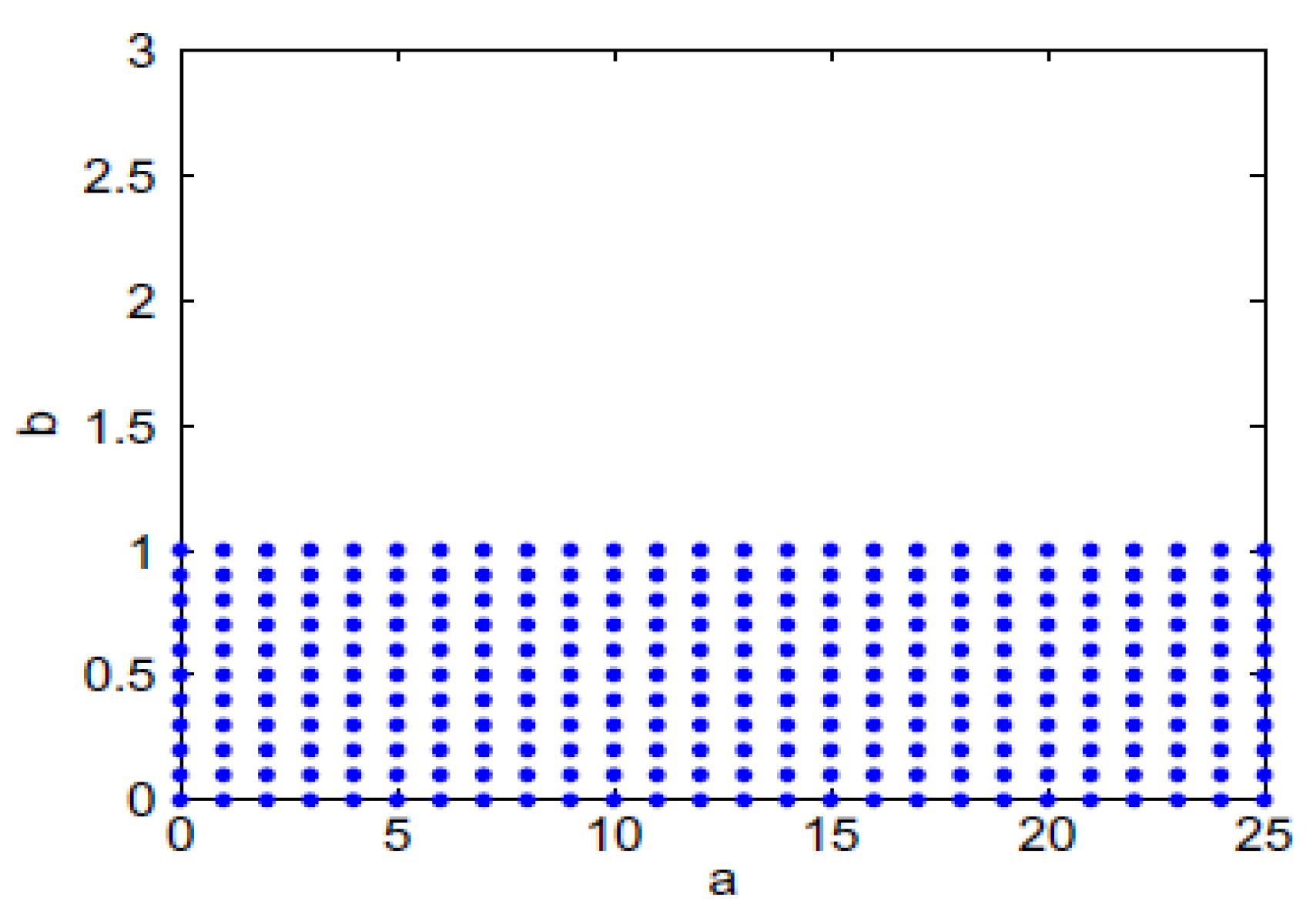
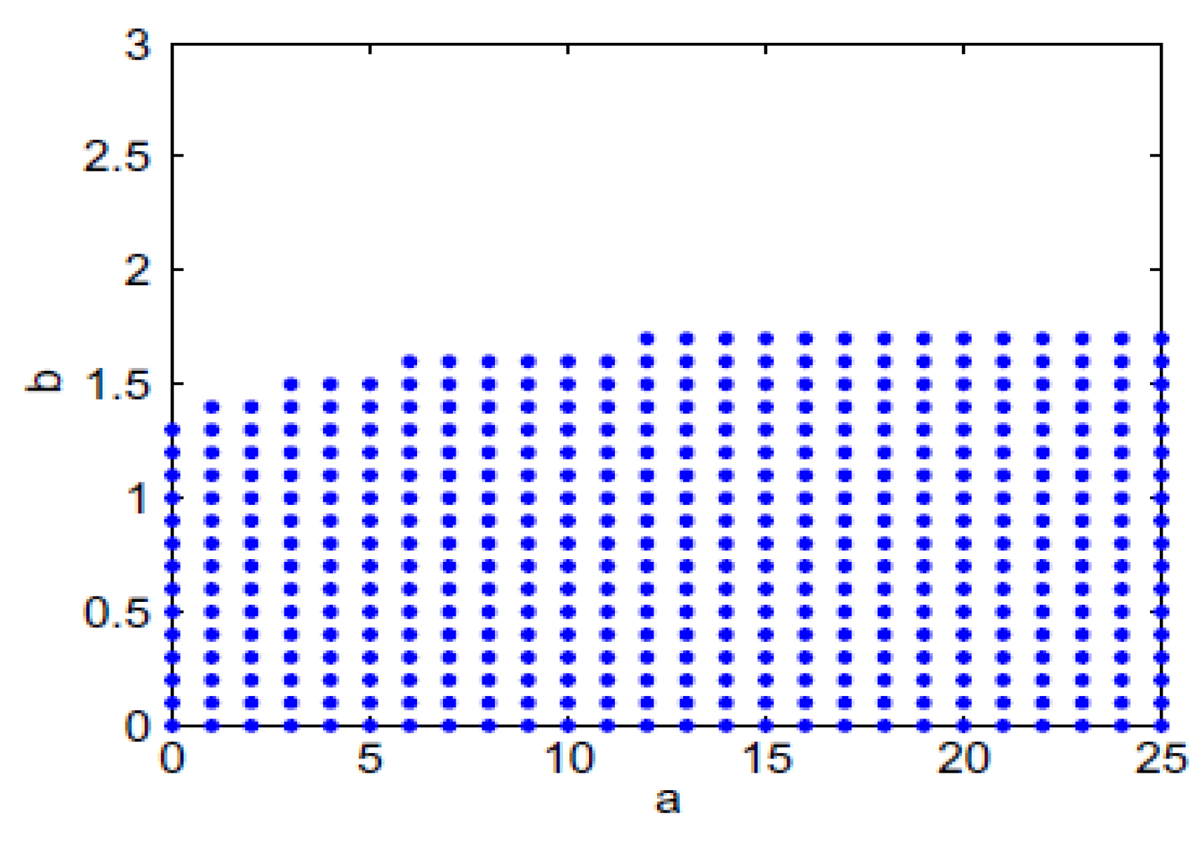
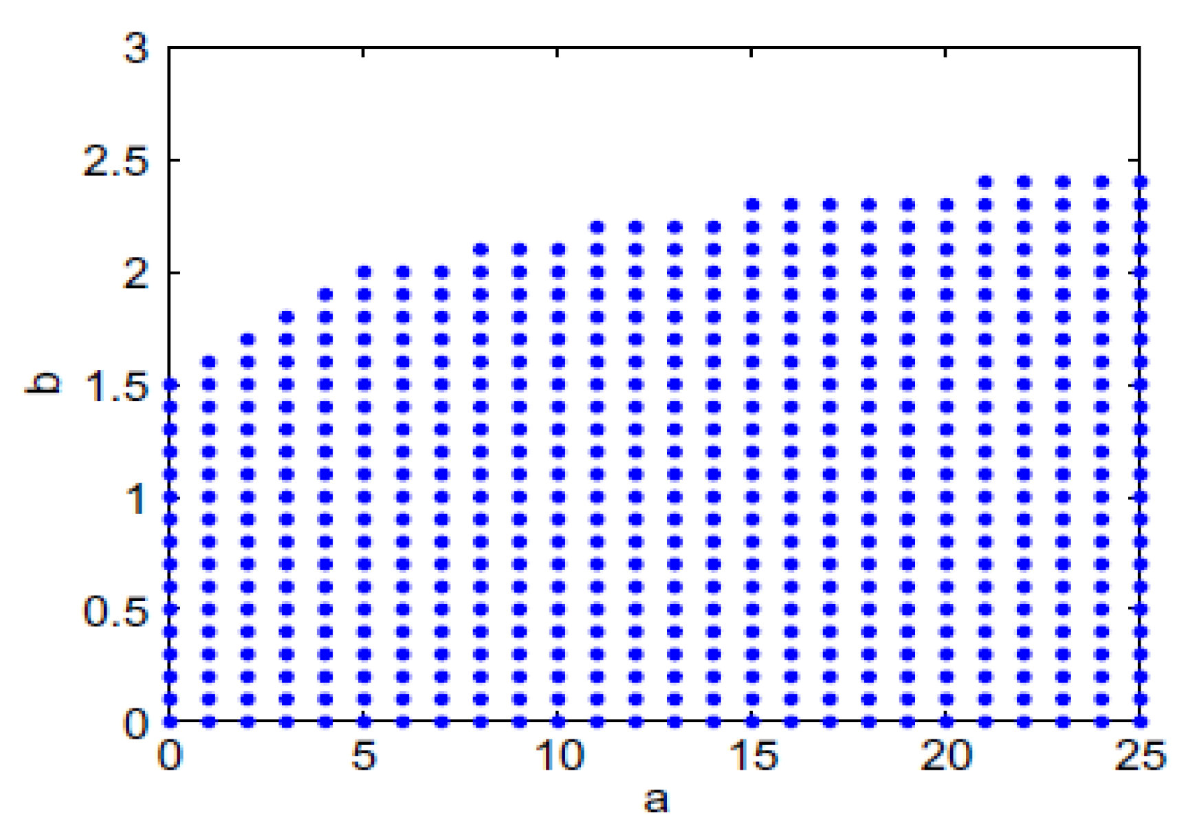
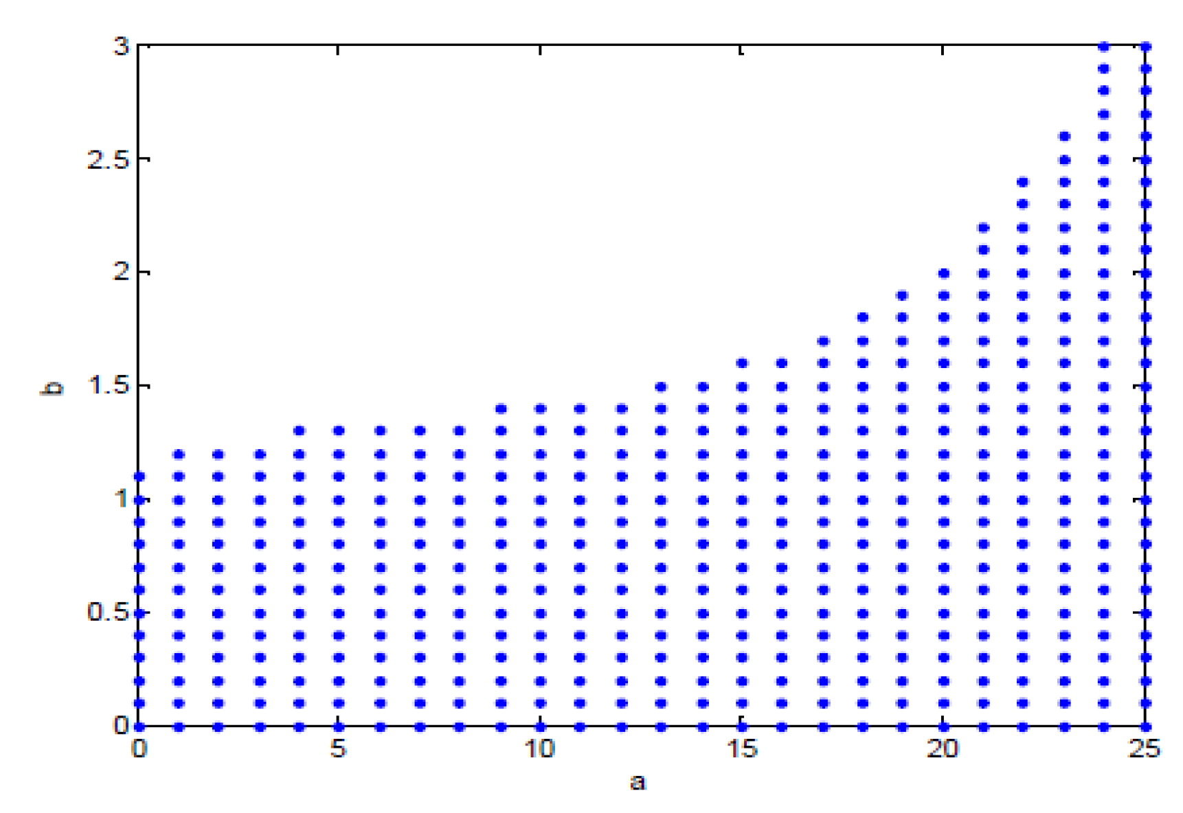
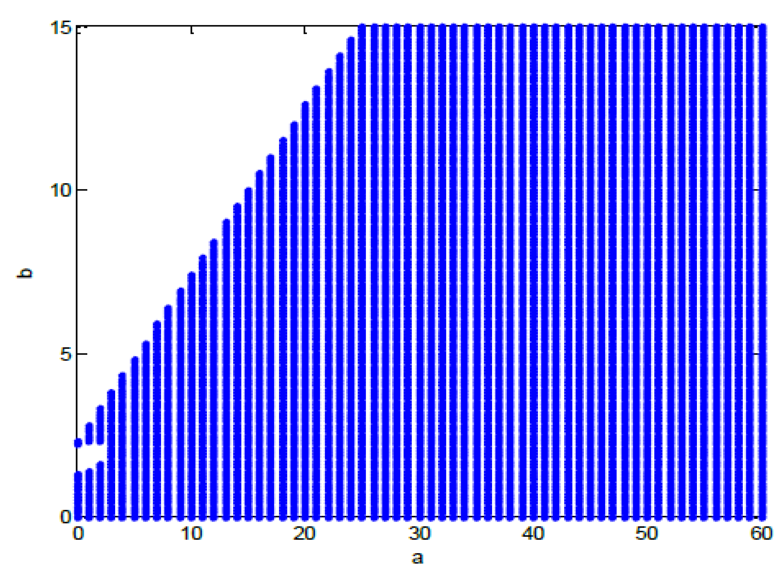
• First step: Using the Euler method, the discrete model corresponding to the continuous model (1) is obtained. Several models were tried, in this case, by progressively increasing the Euler approximation order $m$.
• Second step: By applying Theorem 3 on the previously-obtained discretized model, the discrete gains $F_{di}^{}$ and $H_i$ are determined, satisfying the Euler discrete stabilization model.
• Third step: By saving the previously-obtained gains $F_{di}^{}$ and $H_i$, a new continuous control law, expressed by (20), will be applied to the continuous TS model (1).

  $$u(t)=-F_{dz(t)}^{}\hspace{0.17em}{H}_{z(t)}^{-1}x(t)\hspace{0.17em}\hspace{0.17em}.$$

  (20)

It should be noted that this methodology leads to adopting the function (17) for the Takagi Sugeno continuous models, avoiding BMIs problems at the same time, since some design parameters of the discrete control law were kept.

• Fourth step: By applying the discrete controller, the closed loop continuous TS fuzzy model is expressed by Equation (21):

  $$\dot{x}\left(t\right)=\left(A_{cz\left(t\right)}^{}-B_{cz\left(t\right)}^{}{F}_{dz(t)}^{}{H}_{z\left(t\right)}^{-1}\right)x\left(t\right).$$

  (21)

From Equation (21), the matrices $A_{cz\left(t\right)}^{},\hspace{0.17em}{B}_{cz\left(t\right)}^{},\hspace{0.17em}{F}_{dz\left(t\right)}^{}$, and $H_{z\left(t\right)}^{-1}$ are known, which is considered an advantage. Then, it will be easy to apply the conditions of the SOS approach to check the stability of the model (21), which presents one of the contributions of this research work.

In this case, Theorem 3 is adopted with $A_{pz}^{}=A_{cz}^{}-B_{cz}^{}{F}_{dz}^{}{H}_z^{-1}$, and $T\left(x\right)$ is the identity matrix.

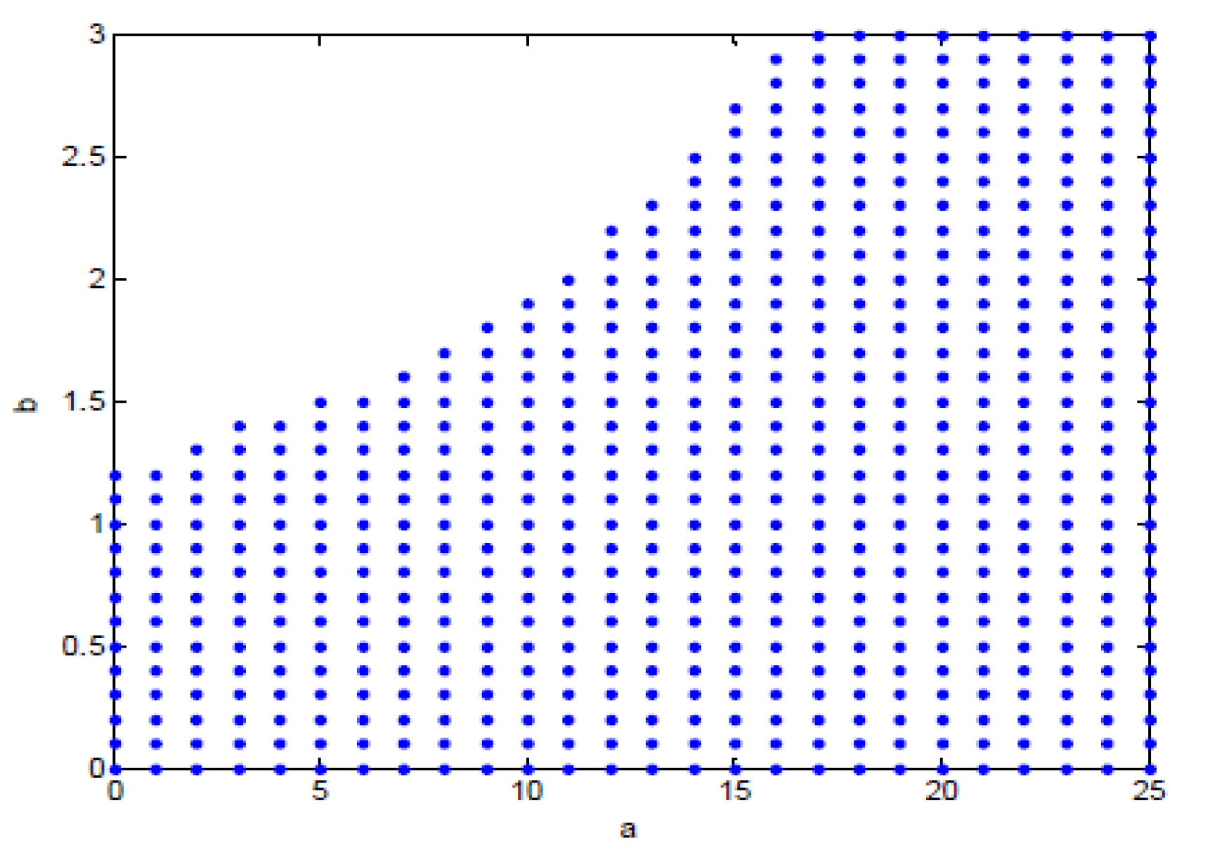
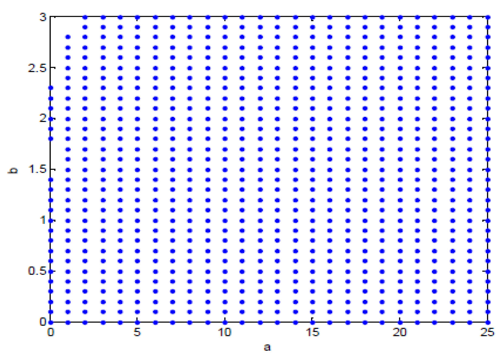
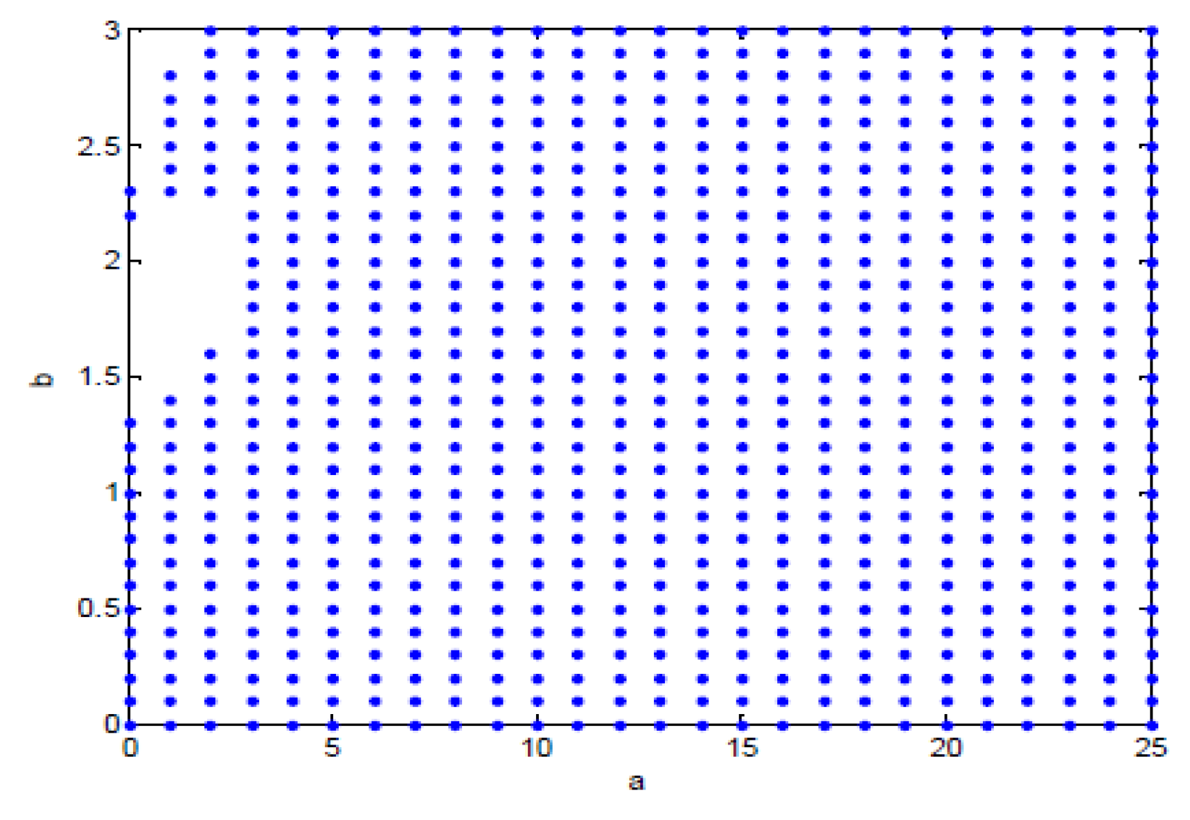
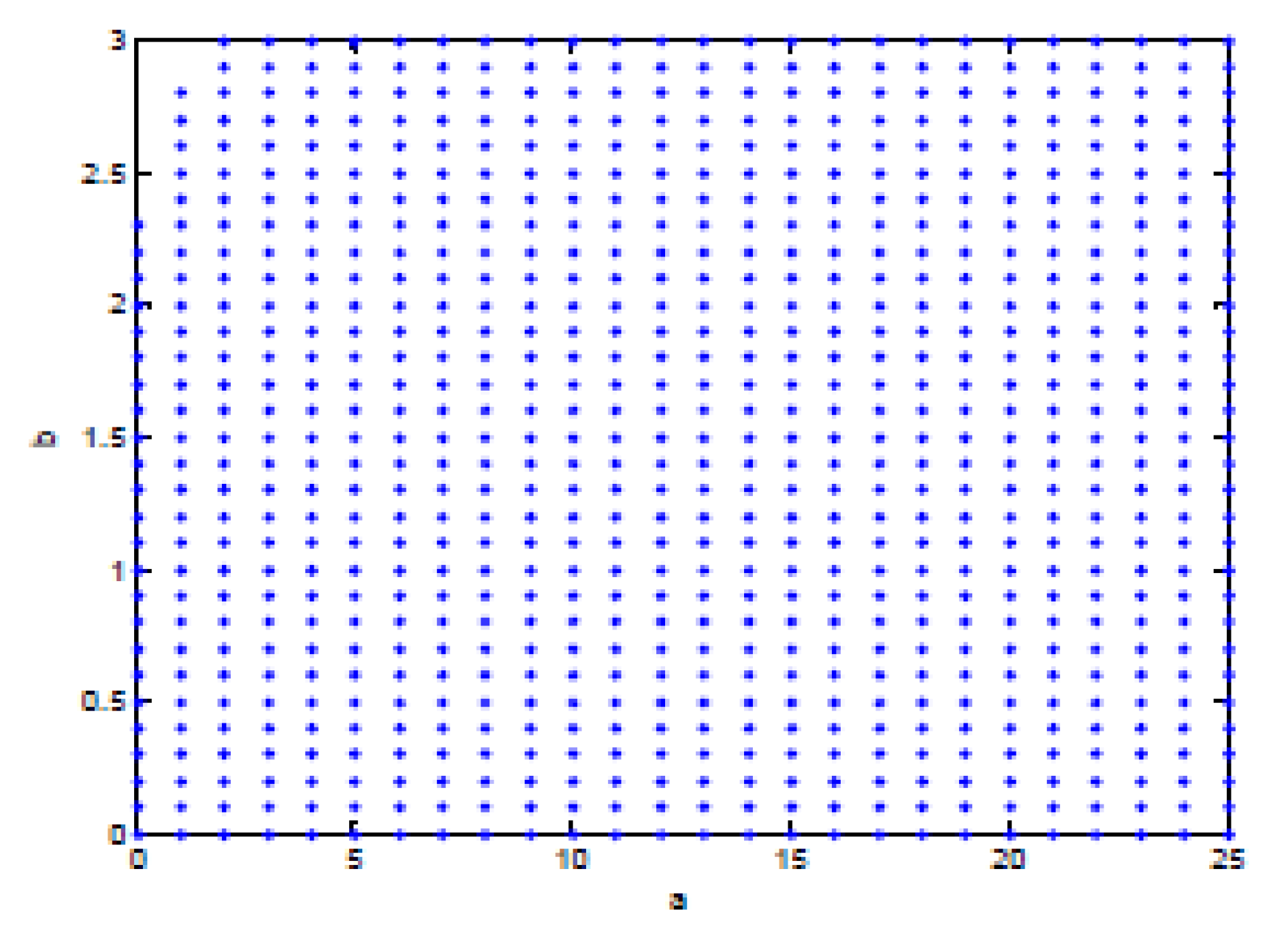
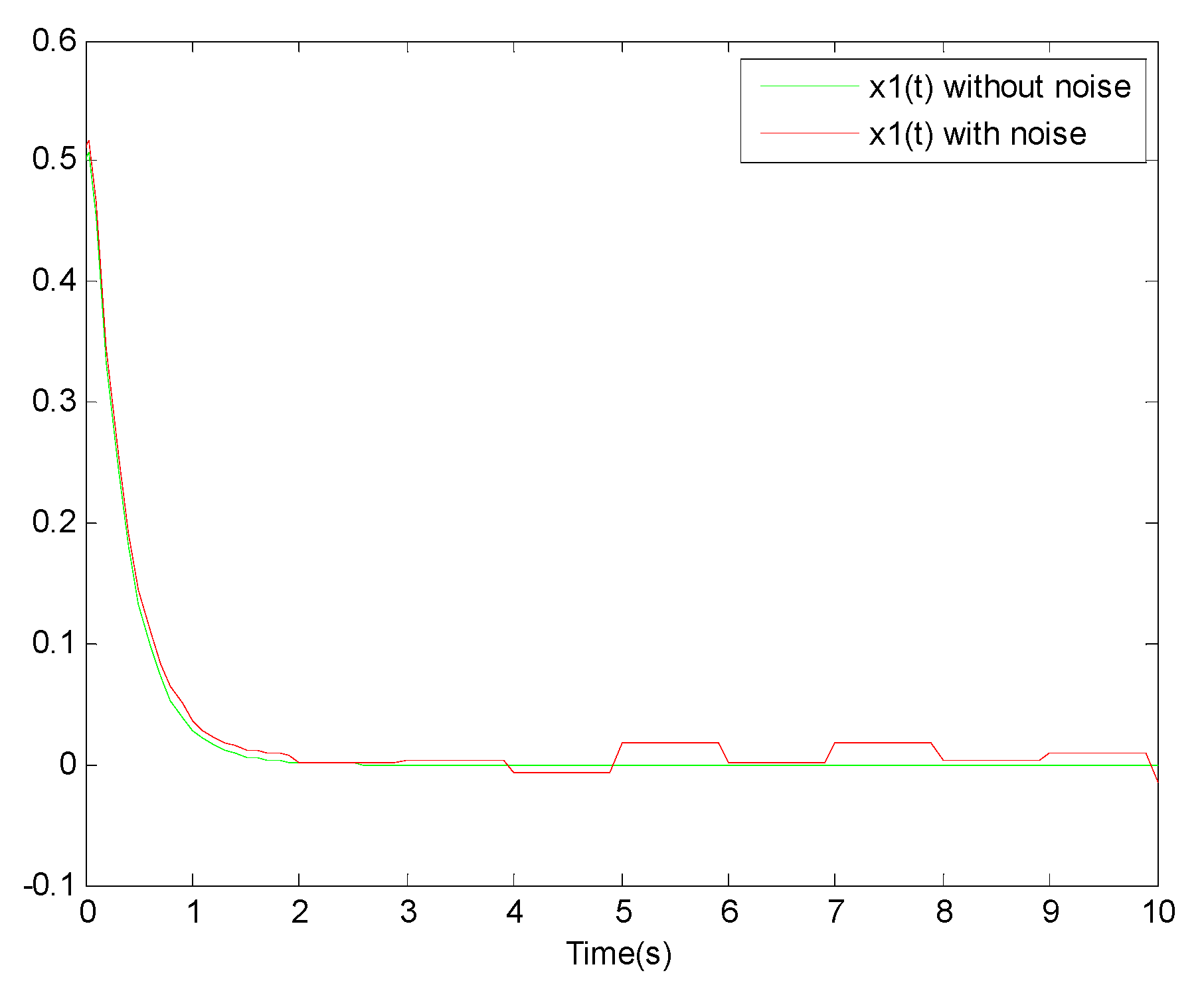
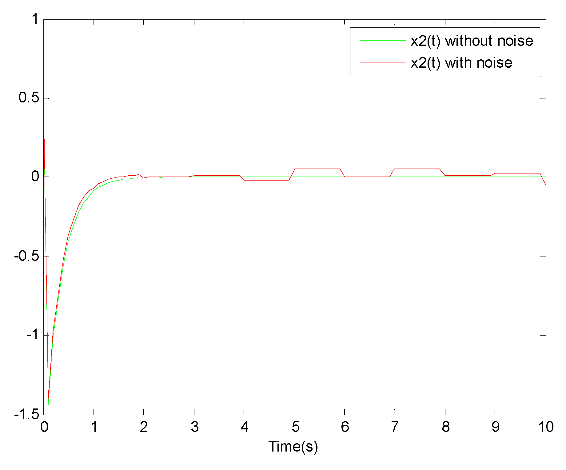
3. Simulation Results and Discussion

After introducing the proposed methodology theoretically, three examples are considered in this section to demonstrate the performance of this proposed idea.

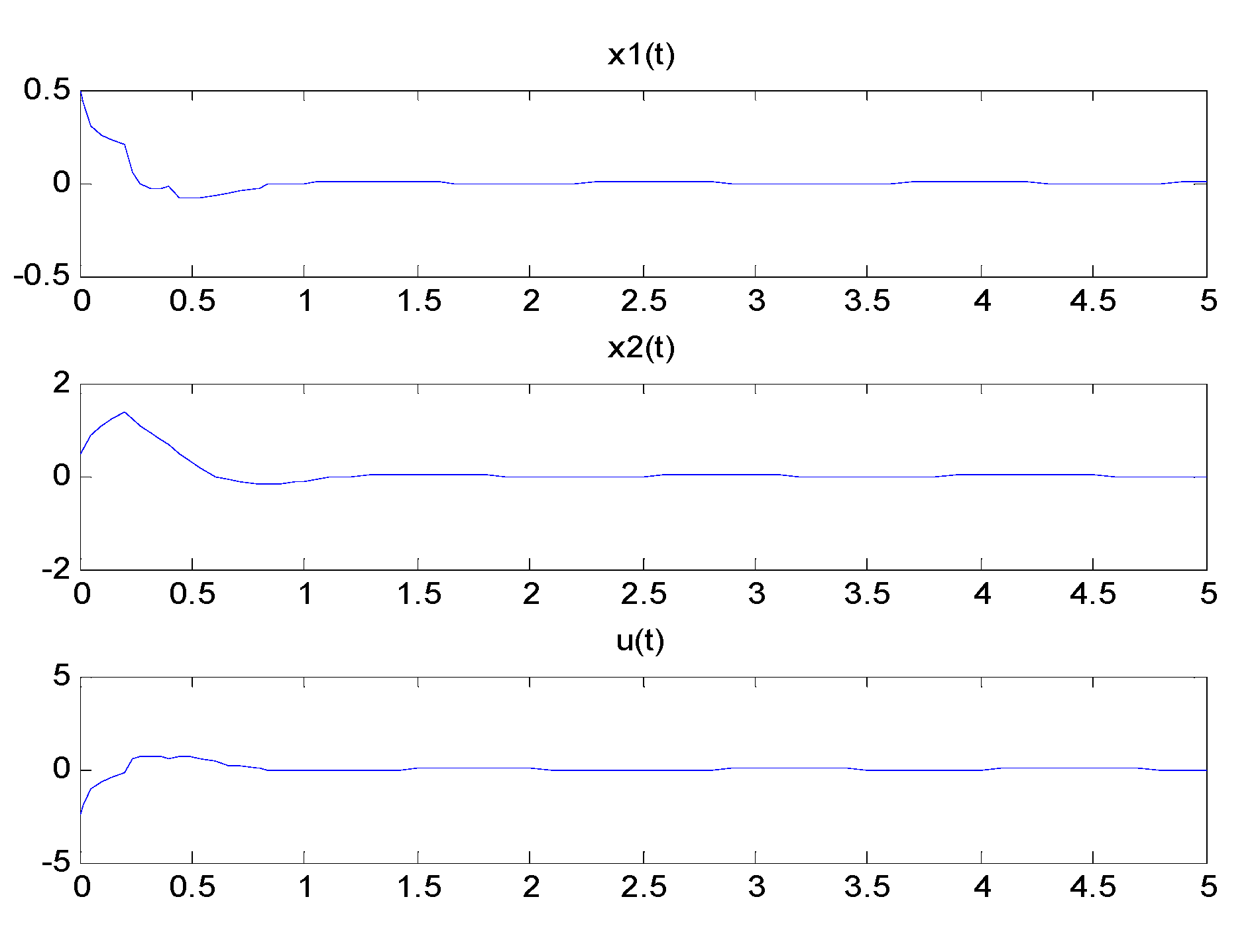
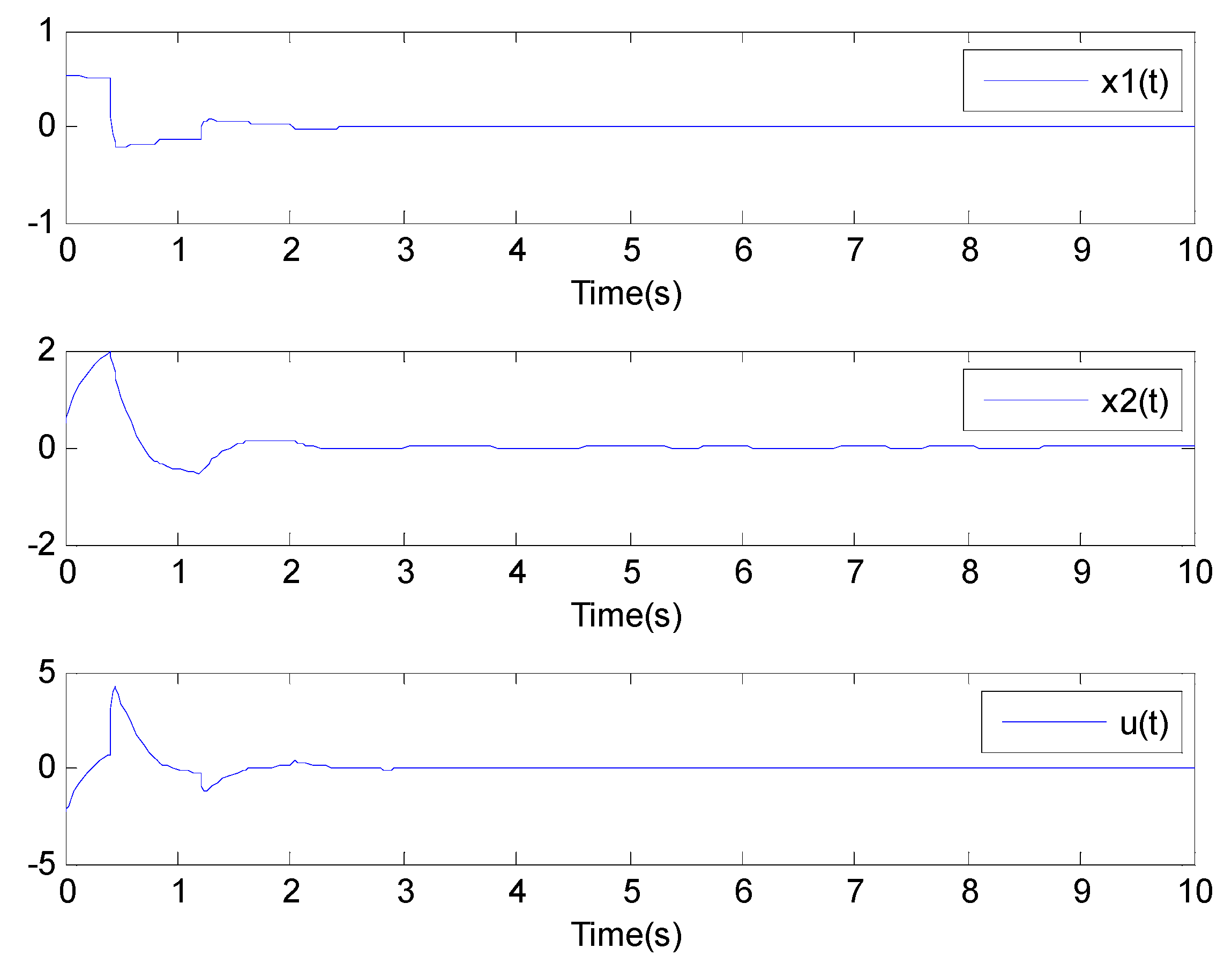
3.1. Example 1

Use the model (22) described by the following matrices [10,28,29]:

$$\begin{array}{l}{A}_{c1}^{}=\left[\begin{array}{cc}3.6& -1.6\\ 6.2& -4.3\end{array}\right], A_{c2}^{}=\left[\begin{array}{cc}-a& -1.6\\ 6.2& -4.3\end{array}\right], B_{c1}^{}=\left[\begin{array}{c}-0.45\\ -3\end{array}\right], B_{c2}^{}=\left[\begin{array}{c}-b\\ -3\end{array}\right]\\ h_1\left(z\left(t\right)\right)=\frac{\sin \left(x_1\left(t\right)\right)}{x_1\left(t\right)}, h_2\left(z\left(t\right)\right)=1-h_1\left(z\left(t\right)\right), -\frac{\pi }{3}\le x_1\left(t\right)\le \frac{\pi }{3}\end{array}.$$

(22)

The closed-loop stability system was checked for several values for the pairs $\left(a,b\right)$. Considering $a\in \left[0,25\right]\hspace{0.17em}$ and $b\in \left[0,1\right]\hspace{0.17em}$, feasible solutions were found by solving the conditions of Theorem 1. As for the Euler discrete system, it was obtained using the Euler approximation (15) and (16). Solving the conditions presented in Theorem 3 leads to feasible solutions for $m\succ 1$ and $b\ge 1$. To expand the solutions feasibility that guarantee the continuous stability model (22), the proposed idea was to apply the previously-described steps. Indeed, $a\in \left[0,25\right]\hspace{0.17em}$ was maintained, and parameter $b$ was adjusted as much as possible to obtain the largest stabilization regions that guarantees the Euler discrete stabilization system. In this case, varying the values of the order $m$ and the sampling period $\delta$ has allowed the study of several models. If the stabilization of the discrete system is guaranteed, it will also be guaranteed for its continuous system. The last step was verified by applying the stability conditions presented in Theorem 2.

Some research works in the literature studied this example for $a\in \left[0,25\right]\hspace{0.17em}$ and $b\in \left[0,3\right]\hspace{0.17em}$ to show the stability region [10,28,29]. Using the proposed methodology for the same values, the feasible solutions can be found for $m\in \left[2,100\right]\hspace{0.17em}$. In this case, it is to highlight that the solutions feasibility depends on the parameter $\delta$ since $\delta$ varies by adjusting $m$. Note that the sampling period $\delta$ is not a constraint to be determined, but it is a parameter to be varied. In our work, the variation of this parameter leads to interesting results because we are able to use large values for the sampling period $\delta$, which is considered to be an advantage for our proposed methodology since faster sampling is usually more difficult to achieve practically, and most of the work existing in the literature has proposed theorems that are only valid for small values of $\delta$, which is seen as a drawback for several authors.

Considering $a\in \left[0,25\right]\hspace{0.17em}$ and $b\in \left[0,3\right]\hspace{0.17em}$,

Table 1. Variation results of $m$ and $\delta$.

$\mathit{m}$	$\mathit{\delta }\left(\mathbf{sec}\right)$
$4$	$\in \left[0.08,0.1\right]$
$10$	$\in \left[0.1,0.2\right]$
$35$	$\in \left[0.2,0.5\right]$
$50$	$\in \left[0.2,0.8\right]$
$70$	$\in \left[0.2,1.1\right]$
$100$	$\in \left[0.2,1.4\right]$

presents the variation results of $m$ and $\delta$.

As shown in Table 1, $\delta$ increases by increasing $m$. By comparing our proposed idea with the existing results in the literature, the stability regions of the continuous model (22) in the plan $a$–$b$ are presented in Figure 1, Figure 2, Figure 3, Figure 4, Figure 5, Figure 6, Figure 7 and Figure 8. Figure 1, Figure 2 and Figure 3 show the existing results:

Based on the proposed idea, Figure 4, Figure 5, Figure 6, Figure 7 and Figure 8 display the stability regions obtained for several values of $m$ and $\delta$ in order to show their influences on the stability results.

Based on the above-displayed figures, and in comparison with the literature, our methodology offers larger stability regions. Furthermore, note that the more the values of $m$ and $\delta$ are increased, the wider the solutions feasibility becomes. Undoubtedly, these figures have demonstrated the merits of increasing the order of approximation on the stability results. The simulation results for the different cases are shown while varying the different parameters.

Case 1: For $a=25$, $b=3$, $m=10$, and $\delta =0.2\hspace{0.17em}\mathrm{s}$, the discrete gains are given by:

$$\begin{array}{l}{F}_{d1}^{}=\left[\begin{array}{cc}0.7058& -54.3352\end{array}\right],\\ F_{d2}^{}=\left[\begin{array}{cc}12.0349& -8.9390\end{array}\right]\end{array}$$

$$\begin{array}{l}{H}_1=\left[\begin{array}{cc}3.0053& 8.0087\\ 10.9714& 42.5153\end{array}\right],\\ H_2=\left[\begin{array}{cc}3.9759& 2.8216\\ 14.7871& 40.3630\end{array}\right].\end{array}$$

Applying the previously-obtained discrete gains, the stability of the continuous model (22) can be checked based on Theorem 3, which leads to feasible solutions given by the following Lyapunov polynomials:

$$P\left(x\right)=\left[\begin{array}{cc}\alpha \left(x\right)& (\ast )\\ \beta \left(x\right)& \sigma \left(x\right)\end{array}\right].$$

• The Lyapunov Polynomials function of the first-order are:

  $$\begin{array}{l}\alpha \left(x\right)=0.1061+0.0874x_1+0.0759x_2\\ \beta \left(x\right)=-0.0128-0.0019x_1-0.0030x_2\\ \sigma \left(x\right)=-0.5036\times {10}^{-3}+0.7617\times {10}^{-3}{x}_1+0.0101x_2\end{array}.$$

Considering the initial conditions presented by $x\left(0\right)=\left[-0.5 0.5\right]$, Figure 9 illustrates the continuous closed-loop results for model (22) controlled by the law in (20).

Figure 9 shows the fast convergence of the Takagi Sugeno continuous system (22). Therefore, it can be noted that the continuous closed loop state response is asymptotically stabilized using the law obtained from the non-PDC controller, satisfying its discrete stabilization model.

Case 2: For $a=25$, $b=3$, $m=100$, and $\delta =0.4$, the discrete gains are given by:

$$\begin{array}{l}{F}_{d1}^{}=\left[\begin{array}{cc}3.7432& -14.6680\end{array}\right],\hspace{0.17em}{F}_{d2}^{}=\left[\begin{array}{cc}0.4117& -15.1675\end{array}\right],\hspace{0.17em}\\ H_1=\left[\begin{array}{cc}2.7966& 7.1999\\ 9.5659& 33.6534\end{array}\right],\hspace{0.17em}{H}_2=\left[\begin{array}{cc}3.0839& 7.3414\\ 8.6791& 32.8930\end{array}\right]\end{array}.$$

The Lyapunov polynomials function of the second-order is given by:

$$\begin{array}{l}\alpha \left(x\right)=0.0356+0.1001x_1+0.1290x_2+0.026639x_1{}^2+0.15508x_1{x}_2+0.7037x_2{}^2\\ \beta \left(x\right)=-0.0090-0.0284x_1-0.0313x_2-0.0072x_1{}^2-0.0531x_1{x}_2-0.1721x_2{}^2\\ \sigma \left(x\right)=0.0013+0.0118x_1+0.0109x_2+0.0042x_1{}^2+0.0145x_1{x}_2+0.0458x_2{}^2\end{array}.$$

Figure 10 shows the stability of the continuous model (22) using the discrete gains.

The feasibility region solutions of the continuous model (22) can be expanded for $a\in \left[0,60\right]\hspace{0.17em}$ and $b\in \left[0,15\right]\hspace{0.17em}$, as shown in Figure 11, Figure 12 and Figure 13. In this case, it is clear that the proposed approach provides larger feasible regions compared to the results of Reference [25], where the stability of the closed-loop system (22) was checked for $a\in \left[0,60\right]\hspace{0.17em}$ and $b\in \left[0,4\right]\hspace{0.17em}$.

As previously stated, the feasibility regions depend on the values of $m$ and $\delta$ since the more the order of Euler approximation is increased, the larger stability region we obtain.

For, $a=60$, $b=15$, $m=100$, and $\delta =0.4\hspace{0.17em}\mathrm{s}$, the following gains are obtained:

$$F_{d1}^{}=\left[\begin{array}{cc}1.8868& -15.4389\end{array}\right],\hspace{0.17em}{F}_{d2}^{}=\left[\begin{array}{cc}2.9929 & -12.1275\end{array}\right]$$

$$H_1=\left[\begin{array}{cc}2.9982& 6.9936\\ 10.7455& 33.1903\end{array}\right],\hspace{0.17em}{H}_2=\left[\begin{array}{cc}3.1588& 8.1046\\ 8.5528& 31.8310\end{array}\right].$$

The Lyapunov polynomials having the order two are given by:

$$\begin{array}{l}\alpha \left(x\right)=0.0735+0.0843x_1+0.0357x_2+0.0412x_1{}^2-0.0512x_1{x}_2+0.1467x_2{}^2\\ \beta \left(x\right)=-0.0177-0.0200x_1-0.0072x_2-0.0091x_1{}^2+0.0115x_1{x}_2-0.0348x_2{}^2\\ \sigma \left(x\right)=-0.0020+0.0195x_1+0.0199x_2+0.0153x_1{}^2-0.0149x_1{x}_2+0.0323x_2{}^2\end{array}.$$

For x(0) = [−0.5, 0.5], the simulations results are shown below, in Figure 14.

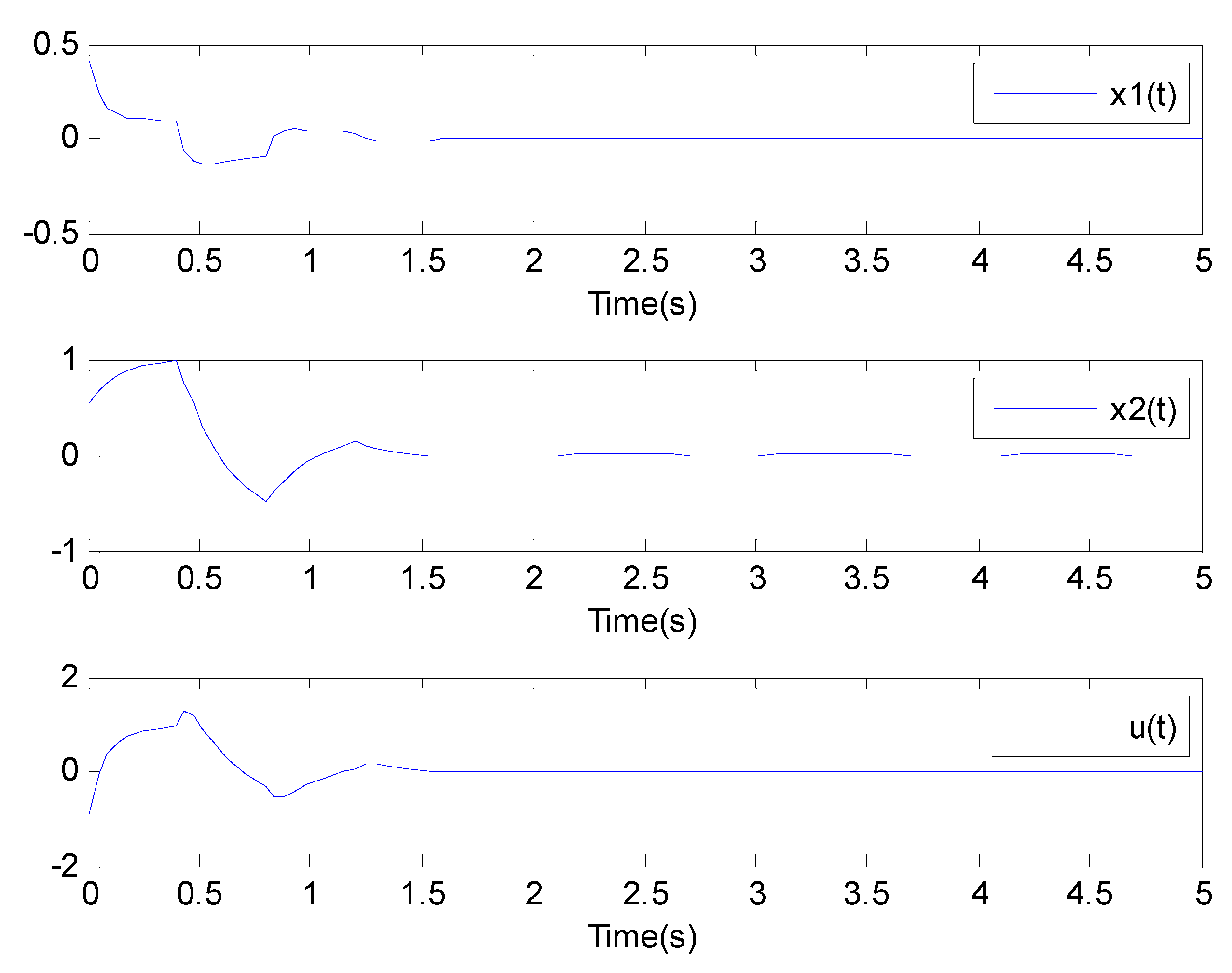
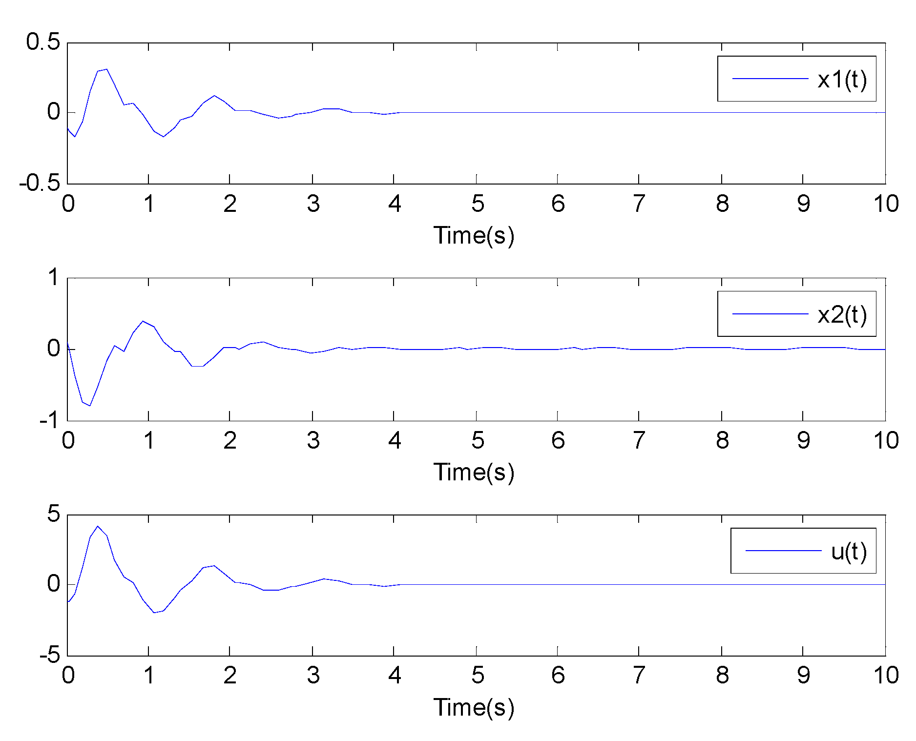
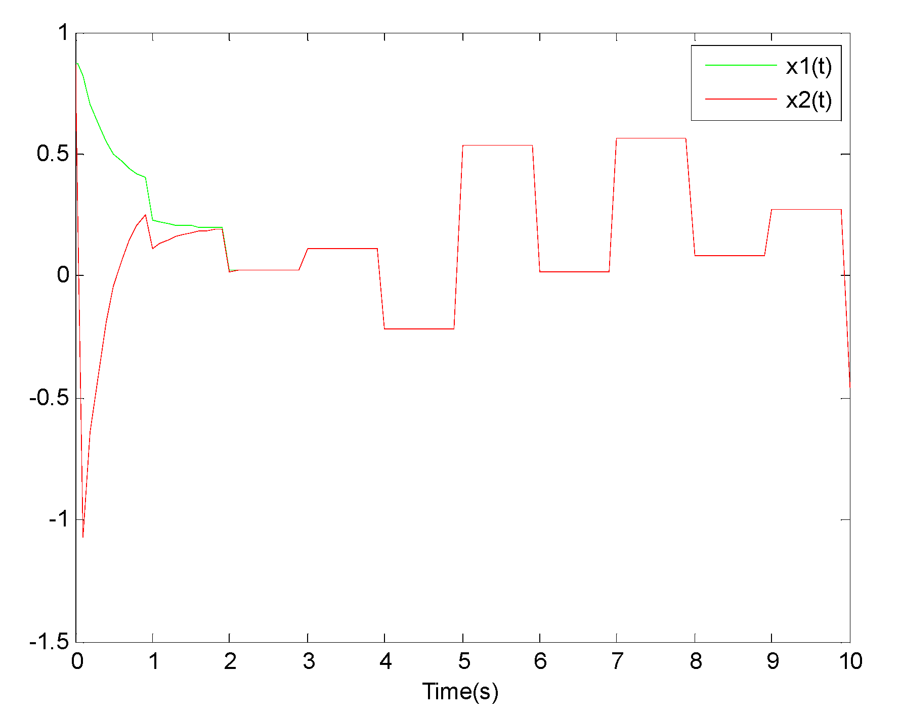
3.2. Example 2

Let us present the following model [30]:

$$\begin{array}{l}{A}_{c1}^{}=\left[\begin{array}{cc}-a& -4\\ -1& -2\end{array}\right], A_{c2}^{}=\left[\begin{array}{cc}-2& -4\\ 20& -2\end{array}\right], B_{c1}^{}=\left[\begin{array}{c}1\\ 10\end{array}\right], B_{c2}^{}=\left[\begin{array}{c}1\\ b\end{array}\right], \\ h_1\left(z\left(t\right)\right)=\frac{1+\sin \left(x_1\left(t\right)\right)}{2}, h_2\left(z\left(t\right)\right)=1-h_1\left(z\left(t\right)\right), -\frac{\pi }{2}\le x_1\left(t\right)\le \frac{\pi }{2}\end{array}.$$

(23)

For $b=1$ and $a\le -4$, the continuous approach based on Theorem 1 does not allow feasible solutions. However, the proposed method in this paper achieved feasible solutions. In fact, for $b=1$, the parameter $a$ can be expanded to $-14$.

Table 2. Feasibility region of solutions of the parameter $a$ related to $m$ and $\delta$.

$\mathit{m}$	$\mathit{\delta }\left(\mathbf{sec}\right)$	$\mathit{a}$
$2$	$0.05$	$\left[-5,\hspace{0.17em}-4\right]$
$10$	$\left[0.05,\hspace{0.17em}0.3\right]$	$\left[-7,\hspace{0.17em}-4\right]$
$20$	$\left[0.05,\hspace{0.17em}0.9\right]$	$\left[-5,\hspace{0.17em}-4\right]$
$50$	$\left[0.05,\hspace{0.17em}1\right]$	$\left[-15,\hspace{0.17em}-4\right]$

below shows some results about the feasibility solutions region of the parameter $a$ related to the variations of $m$ and $\delta$. It should be noted that any feasible solution was found with the first order of approximation.

From Table 2, it can be concluded that the more the value of $m$ increases, the larger the feasibility region of the solutions of parameter $a$ becomes.

This interesting result was validated by the application of the stability conditions from Theorem 3 to verify the continuous stability of the model (23) using the discrete gains.

Let us consider the case of $b=1$, $a=-14$, $m=50$, and $\delta =0.7\hspace{0.17em}\mathrm{s}$, and the Lyapunov polynomials function of order two is given by:

$$\begin{array}{l}\alpha \left(x\right)=0.6649+0.7296x_1+0.3991x_2+0.5293x_1{}^2-0.0317x_1{x}_2+1.4384x_2{}^2\\ \beta \left(x\right)=-0.1620-0.1668x_1-0.0850x_2-0.1198x_1{}^2+0.1952{\times 10}^{-3}{x}_2{x}_1-0.331x_2\\ \sigma \left(x\right)=0.0351+0.0474x_1+0.0265x_2+0.0335x_1{}^2-0.0036x_1{x}_2+0.0863x_2{}^2\end{array}.$$

Figure 15 presents the continuous closed loop curves for the model (23) controlled by the discrete law and using $x(0)=\left[\begin{array}{cc}-0.1& 0.1\end{array}\right]\hspace{0.17em}$.

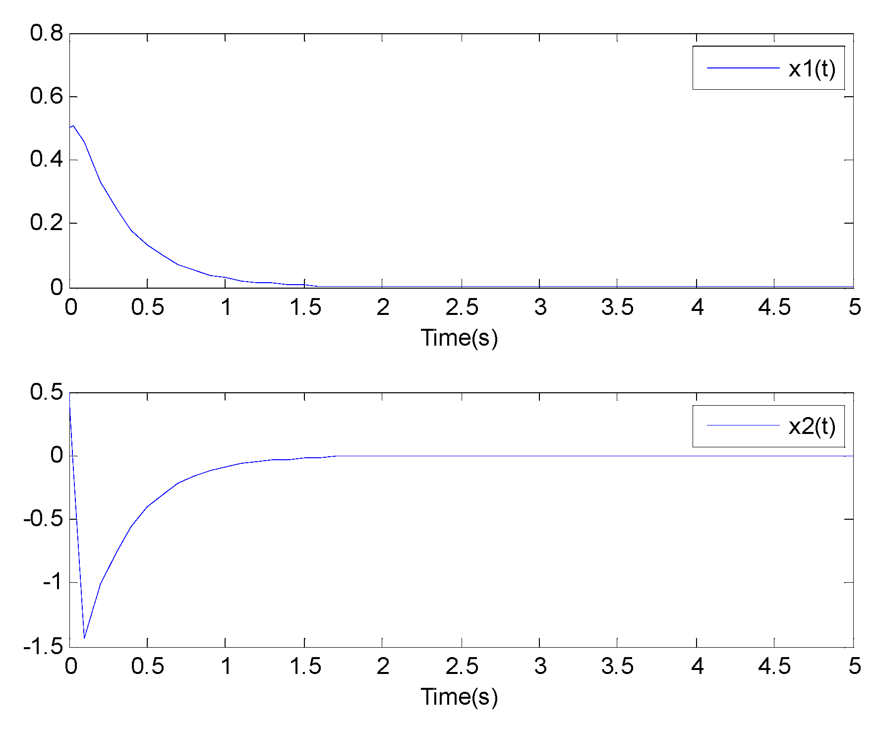
3.3. Example 3

The following example is presented to illustrate the applicability of our proposed methodology. Consider the problem of balancing and swing-up of an invented pendulum on a cart. The dynamics of its non-linear model is given by the following equations [31]:

$$\{\begin{array}{l}\stackrel{•}{{{\displaystyle x}}_1}\left(t\right)={{\displaystyle x}}_2\left(t\right)\\ \stackrel{•}{{{\displaystyle x}}_2}\left(t\right)=\frac{g\hspace{0.17em}\sin \left({{\displaystyle x}}_1\left(t\right)\right)-aml{{\displaystyle x}}_2{\left(t\right)}^2\frac{\sin \left(2{{\displaystyle x}}_1\left(t\right)\right)}{2}-a\cos \left({{\displaystyle x}}_1\left(t\right)\right)u\left(t\right)}{\frac{4l}{3}-aml\cos {\left({{\displaystyle x}}_1\left(t\right)\right)}^2}\end{array},$$

(24)

where ${{\displaystyle x}}_1\left(t\right)$ is the angle of the pendulum from the vertical, ${{\displaystyle x}}_2\left(t\right)$ is the angular velocity, and $u\left(t\right)$ is the force applied to the cart.

• $M$ cart mass $\left(20\hspace{0.17em}\hspace{0.17em}\mathrm{kg}\right)$,
• $m$ pendulum mass $\left(0.025\hspace{0.17em}\hspace{0.17em}\mathrm{kg}\right)$,
• g gravity constant $\left(9.81\hspace{0.17em}\mathrm{m}\cdot {\mathrm{s}}^{-2}\right)$,
• $2l$ length of the pendulum $\left(1\hspace{0.17em}\hspace{0.17em}\mathrm{m}\right)$.

The continuous TS fuzzy model is presented by the following matrices:

$$\begin{array}{l}{A}_{c1}=\left[\begin{array}{cc}0& 1\\ \frac{g}{\frac{4l}{3}-aml}& 0\end{array}\right],\hspace{0.17em}\hspace{0.17em}\hspace{0.17em}{B}_{c1}=\left[\begin{array}{c}0\\ -\frac{a}{\frac{4l}{3}-aml}\end{array}\right]\\ A_{c2}=\left[\begin{array}{cc}0& 1\\ \frac{g}{\pi \left(\frac{4l}{3}-aml\right){\beta }^2}& 0\end{array}\right],\hspace{0.17em}\hspace{0.17em}\hspace{0.17em}{B}_{c2}=\left[\begin{array}{c}0\\ -\frac{a\beta }{\frac{4l}{3}-aml{\beta }^2}\end{array}\right]\end{array},$$

(25)

where $a=\frac{1}{m+M}$ and $\beta =\cos \left(\frac{\pi }{2}\right)$.

For the above parameters, the continuous approach based on Theorem 1 does not allow feasible solutions. The discretized model of the fuzzy continuous model (25) is obtained using the Euler approximation. This approximation is performed for various orders. In this context, various models are studied, and several tests are carried out that allow determining, for each model, the adequate value of the sampling period $\delta$ that guarantees the feasibility solutions. For example, for $m=2$ and $\delta =0.2$, the discrete gains are given by:

$$F_{d1}^{}=\left[\begin{array}{cc}-1.7584& -6.5252\end{array}\right], F_{d2}^{}=\left[\begin{array}{cc}-1.5607 & -5.9628\end{array}\right]$$

$$H_1=\left[\begin{array}{cc}0.5345& -0.0942\\ -0.7407 & 4.4138\end{array}\right], H_2=\left[\begin{array}{cc}0.2601& -0.7958\\ -0.7958& 2.4344\end{array}\right].$$

Applying the previously-obtained discrete gains, the stability of the continuous model (25) can be checked based on Theorem 3, which leads to feasible solutions given by the following Lyapunov Polynomials function of the first-order:

$$\begin{array}{l}\alpha \left(x\right)=0.0738+0.1694x_1+0.1760x_2\\ \beta \left(x\right)=-0.0186-0.0459x_1-0.0436x_2\\ \sigma \left(x\right)=0.0037+0.0162x_1+0.0141x_2\end{array}.$$

Figure 16 presents the continuous closed loop curves for the model (25) controlled by the discrete law using x(0) = [−0.5, 0.5].

From Figure 16, it can be proved that the evolutions of the state response, driven by the discrete controller, lead to interesting results regarding their fast stabilization.

To evaluate the stability performance of the discrete controller, a white Gaussian noise is applied to the states of the pendulum. This noise is characterized by the variance σ. The value of σ is varied until the system loses its stability performance. Figure 17 and Figure 18 are obtained.

Figure 19 shows that the system loses its stability performance for σ = 0.1.

4. Conclusions

The stability results in the continuous case suffer from conservatism since it is still quite difficult to use the non-quadratic Lyapunov functions, while it is much easier in the discrete case. To overcome such a problem, a novel method of stability analysis for the continuous systems was proposed using the controller obtained from the Euler discretized model. Using this control law, the SOS approach was adopted to check the stability of continuous systems with discrete gains.

The simulation results showed the advantage of the Euler method with greater order of approximation. Indeed, the higher the order of approximation is, the longer the sampling period is augmented, and the solutions’ feasibility becomes guaranteed. Consequently, the stability regions became broader. The results proved the Euler method influence on the continuous stability regions, which was checked on the basis of SOS stability conditions. Indeed, the stability of the continuous models could be guaranteed using the obtained discrete controller and the Lyapunov polynomial function. This stability could not have been guaranteed using the classical quadratic Lyapunov function since it leads to BMI. In this case, the non PDC control law can be used in the continuous case, and, consequently, the BMIs problems are avoided, and the LMI drawbacks using the non-quadratic approaches are overcome.

References

- Takagi, G.T.; Sugeno, M. Fuzzy identification of systems and its applications to modeling and control. IEEE Trans. SMC 1985, 15, 116–132. [Google Scholar] [CrossRef]
- Tuan, H.D.; Apkarian, P.; Narikiyo, T.; Yamamoto, Y. Parameterized linear matrix inequality techniques in Fuzzy control system design. IEEE Trans. Fuzzy Syst. 2001, 19, 324–332. [Google Scholar] [CrossRef] [Green Version]
- Tanaka, K.; Hori, T.; Wang, H.O. A multiple Lyapunov function approach to stabilization of fuzzy control systems. IEEE Trans. Fuzzy Syst. 2003, 11, 582–589. [Google Scholar] [CrossRef]
- Guerra, T.M.; Vermeiren, L. LMI-based relaxed nonquadratic stabilization conditions for nonlinear systems in the Takagi-Sugeno’s form. Automatica 2004, 40, 823–829. [Google Scholar] [CrossRef]
- Tanaka, K.; Wang, H.O. Fuzzy Control Systems Design and Analysis. A Linear Matrix Inequality Approach; John Wiley and Sons: Hoboken, NJ, USA, 2001. [Google Scholar]
- Ding, B.C.; Sun, H.X.; Yang, P. Further studies on LMI-based relaxed stabilization conditions for nonlinear systems in Takagi-Sugeno’s form. Automatica 2006, 42, 503–508. [Google Scholar] [CrossRef]
- Salah, R.B.; Kahouli, O.; Hadjabdallah, H.A. Nonlinear Takagi-Sugeno fuzzy logic control for single machine power system. Int. J. Adv. Manuf. Technol. 2017, 90, 575–590. [Google Scholar] [CrossRef]
- Chen, Y.J.; Ohtake, H.; Tanaka, K.; Wang, W.J.; Wang, H.O. Relaxed Stabilization Criterion for T-S Fuzzy Systems by Minimum-type Piecewise Lyapunov Function Based Switching Fuzzy Controller. IEEE Trans. Fuzzy Syst. 2012, 20, 1166–1173. [Google Scholar] [CrossRef]
- Pan, J.T.; Guerral, T.M.; Fei, S.M.; Jaadari, A. Non Quadratic Stabilization of Continuous TS Fuzzy Models: LMI Solution for a Local Approach. IEEE Trans. Fuzzy Syst. 2012, 20, 1063–6706. [Google Scholar] [CrossRef]
- Chang, X.H.; Yang, G.H. Relaxed stabilization conditions for continuous-time Takagi-Sugeno fuzzy control systems. Inf. Sci. 2010, 180, 3273–3287. [Google Scholar] [CrossRef]
- Bernal, M.; Husek, P.; Kucera, V. Nonquadratic stabilization of continuous-time systems in the Takagi-Sugeno form. Kybernetika 2006, 42, 665–672. [Google Scholar]
- Vafamand, N. Global non-quadratic Lyapunov-based stabilization of T-S fuzzy systems: A descriptor approach. J. Vib. Control 2020, 26, 1765–1778. [Google Scholar] [CrossRef]
- Cao, Y.; Frank, P.M.; Hadjili, M.L. Stability analysis and synthesis of nonlinear time-delay systems via linear Takagi-Sugeno fuzzy models. Fuzzy Sets Syst. 2001, 124, 213–229. [Google Scholar] [CrossRef]
- Cao, Y.; Frank, P.M.; Hadjili, M.L. Improved delay-dependent robust stabilization conditions of uncertain T-S fuzzy systems with time-varying delay. Fuzzy Sets Syst. 2008, 159, 2713–2729. [Google Scholar]
- Ellouze, A.; Lauber, J.F.; Delmotte Chtourou, M.; Ksantini, M. Non quadratic Lyapunov function for continuous TS fuzzy models through their discretized forms. Fuzzy Sets Syst. 2014, 253, 64–81. [Google Scholar] [CrossRef]
- Ellouze, A.; Lauber, J.; Delmotte, F.; Chtourou, M.; Ksantini, M. On the stabilization of continuous fuzzy models using their discretized forms. In Proceedings of the 20th Mediterranean Conference on Control & Automation (MED), Barcelona, Spain, 3–6 July 2012; pp. 3–6. [Google Scholar]
- Prajna, S.; Papachristodoulou, A.; Wu, F. Nonlinear control synthesis by sum of squares optimization: A Lyapunov-based approach. In Proceedings of the Asian Control Conference (ASCC), Melbourne, Australia, 20–23 July 2004; pp. 157–165. [Google Scholar]
- Tanaka, K.; Yoshida, H.; Othake, H.; Wang, H.O. A sum-of-squares approach to modeling and control of nonlinear dynamical systems with polynomial fuzzy systems. IEEE Trans. Fuzzy Syst. 2009, 17, 911–922. [Google Scholar] [CrossRef]
- Guelton, K.; Manamanni, N.; Koumba-Emianiwe, D.L.; Chinh, C.D. SOS stability conditions for nonlinear systems based on a polynomial fuzzy Lyapunov function. In Proceedings of the 18th IFAC World Congress, Milano, Italy, 29 August–3 September 2011; Volume 18, pp. 12777–12782. [Google Scholar]
- Lam, H.K.; Li, H. Output-feedback tracking control for polynomial fuzzy-model-based control systems. IEEE Trans. Ind. Electron. 2013, 60, 5830–5840. [Google Scholar] [CrossRef]
- Lam, H.K.; Wu, L.; Lam, J. Two-step stability analysis for general polynomial-fuzzy-model-based control systems. IEEE Trans. Fuzzy Syst. 2015, 23, 511–524. [Google Scholar] [CrossRef] [Green Version]
- Rakhshan, M.; Vafamand, N.; Mardani, M.M. Polynomial control design for polynomial systems: A non-iterative sum of squares approach. Trans. Inst. Meas. Control 2018, 41, 1993–2004. [Google Scholar] [CrossRef]
- Zhao, D.Y.; He, Y.; Du, X. Relaxed Sum-of-Squares Based Stabilization Conditions for Polynomial Fuzzy-Model-Based Control Systems. IEEE Trans. Fuzzy Syst. 2019, 27, 1767–1778. [Google Scholar] [CrossRef]
- Chaibi, R.; Hmamed, A.; Tissir, E.H.; Tadeo, F. Control of Discrete 2-D Takagi-Sugeno Systems Via a Sum-Of-Squares Approach. J. Control Autom. Electr. Syst. 2019, 30, 137–147. [Google Scholar] [CrossRef]
- Wang, H.O.; Tanaka, K.; Griffin, M. An approach to fuzzy control of non linear systems: Stability and design issues. IEEE Trans. Fuzzy Syst. 1996, 4, 14–23. [Google Scholar] [CrossRef]
- Prajna, S.; Papachristodoulou, A.; Parrilo, P.A. Introducing SOSTOOLS: A general purpose sum of squares programming solver. In Proceedings of the IEEE Conference on Decision and Control, Las Vegas, NV, USA, 12–14 December 2002. [Google Scholar]
- Nesic, D.; Teel, A.R.; Kokotovic, P.V. Sufficient conditions for stabilization of sampled-data nonlinear systems via discrete-time approximations. Syst. Contr. Lett. 1999, 38, 259–270. [Google Scholar] [CrossRef] [Green Version]
- Mozelli, L.A.; Palhares, R.M.; Avellar, G.S.C. A systematic approach to improve multiple Lyapunov function stability and stabilization conditions for fuzzy systems. Inf. Sci. 2009, 179, 1149–1162. [Google Scholar] [CrossRef]
- Bernal, M.; Guerra, T.M.; Jaadari, A. Non quadratic stabilization of Takagi Sugeno models: A local point of view. In Proceedings of the International Conference on Fuzzy Systems, Luxembourg, 11–14 July 2010. [Google Scholar]
- Lee, D.H.; Park, J.B.; Joo, Y.H. Fuzzy Lyapunov function approach to estimating the domain of attraction for continuous-time Takagi-Sugeno fuzzy systems. Inf. Sci. 2012, 185, 230–248. [Google Scholar] [CrossRef]
- Huijun, G.; Tongwen, C. Stabilization of Nonlinear Systems Under Variable Sampling: A Fuzzy Control Approach. IEEE Trans. Fuzzy Syst. 2007, 185, 972–983. [Google Scholar]
Publisher’s Note: MDPI stays neutral with regard to jurisdictional claims in published maps and institutional affiliations. |
© 2021 by the authors. Licensee MDPI, Basel, Switzerland. This article is an open access article distributed under the terms and conditions of the Creative Commons Attribution (CC BY) license (https://creativecommons.org/licenses/by/4.0/).
Share and Cite
Ellouze, A.; Kahouli, O.; Ksantini, M.; Rebhi, A.; Hnaien, N.; Delmotte, F. Continuous Stability TS Fuzzy Systems Novel Frame Controlled by a Discrete Approach and Based on SOS Methodology. Mathematics 2021, 9, 3129. https://doi.org/10.3390/math9233129
Ellouze A, Kahouli O, Ksantini M, Rebhi A, Hnaien N, Delmotte F. Continuous Stability TS Fuzzy Systems Novel Frame Controlled by a Discrete Approach and Based on SOS Methodology. Mathematics. 2021; 9(23):3129. https://doi.org/10.3390/math9233129
Chicago/Turabian StyleEllouze, Ameni, Omar Kahouli, Mohamed Ksantini, Ali Rebhi, Nidhal Hnaien, and François Delmotte. 2021. "Continuous Stability TS Fuzzy Systems Novel Frame Controlled by a Discrete Approach and Based on SOS Methodology" Mathematics 9, no. 23: 3129. https://doi.org/10.3390/math9233129