
Mixture of Species Sampling Models

Department of Mathematics, Politecnico of Milano, 20133 Milano, Italy
*
Author to whom correspondence should be addressed.
†
These authors contributed equally to this work.
Mathematics 2021, 9(23), 3127; https://doi.org/10.3390/math9233127
Submission received: 5 November 2021
/
Revised: 30 November 2021
/
Accepted: 2 December 2021
/
Published: 4 December 2021
(This article belongs to the Special Issue Bayesian Predictive Inference and Related Asymptotics—Festschrift for Eugenio Regazzini's 75th Birthday)
Abstract
:We introduce mixtures of species sampling sequences (mSSS) and discuss how these sequences are related to various types of Bayesian models. As a particular case, we recover species sampling sequences with general (not necessarily diffuse) base measures. These models include some “spike-and-slab” non-parametric priors recently introduced to provide sparsity. Furthermore, we show how mSSS arise while considering hierarchical species sampling random probabilities (e.g., the hierarchical Dirichlet process). Extending previous results, we prove that mSSS are obtained by assigning the values of an exchangeable sequence to the classes of a latent exchangeable random partition. Using this representation, we give an explicit expression of the Exchangeable Partition Probability Function of the partition generated by an mSSS. Some special cases are discussed in detail—in particular, species sampling sequences with general base measures and a mixture of species sampling sequences with Gibbs-type latent partition. Finally, we give explicit expressions of the predictive distributions of an mSSS.
1. Introduction
Discrete random measures have been widely used in Bayesian nonparametrics. Noteworthy examples of such random measures are the Dirichlet process [1], the Pitman–Yor process [2,3], (homogeneous) normalized random measures with independent increments (see, e.g., [4,5,6,7]), Poisson–Kingman random measures [8] and stick-breaking priors [9]. All the previous random measures are of the form
where are i.i.d. random variables taking values in a Polish space with common distribution H, and are random positive weights in , independent of , such that .
With a few exceptions—see, e.g., [1,4,10,11,12,13,14]—the base measure H of a random measure P in (1) is usually assumed to be diffuse, since this simplifies the derivation of various analytical results.
The diffuseness of H is assumed also to define the so-called species sampling sequences [15], exchangeable sequences whose directing measure is a discrete random probability of type (1). In this case, the diffuseness of H is motivated by the interpretation of species sampling sequences as sequences describing a sampling mechanism in discovering species from an unknown population. In this context, the s are the possible infinite different species, and the diffuseness of H ensures that there is no redundancy in this description.
On the other hand, from a Bayesian point of view, the diffuseness of H is not always reasonable and there are situations in which a discrete (or mixed) H is indeed natural. For example, recent interest in species sampling models with a spike-and-slab base measure emerged in [16,17,18,19,20,21] in order to induce sparsity and facilitate variable selection. Other models, which are implicitly related to species sampling sequences with non-diffused base measures, are mixtures of Dirichlet processes [10] and hierarchical random measures; see, e.g., [22,23,24,25].
The combinatorial structure of species sampling sequences derived from random measure (1) with general H have been recently studied in [14].
In this paper, we discuss some relevant properties of species sampling sequences with general base measures, as well as some further generalizations, namely mixtures of species sampling sequences with general base measures (mSSS).
An mSSS is an exchangeable sequence whose directing random measure is of type (1), where is a sequence of exchangeable random variables and are random positive weights in with , independent of .
The core of the results that we prove in this paper is that all the mSSS can be obtained by assigning the values of an exchangeable sequence to the classes of a latent exchangeable random partition. We summarize the results of Section 3 in the next statement.
The following are equivalent:
- is an mSSS;
- with probability one , where is a sequence of integer-valued random variables independent of the Zs such that, conditionally on , the are independent and .
- with probability one , where is an exchangeable sequence with the same law of , Π is an exchangeable partition, independent of , obtained by sampling from , and is the index of the block in Π containing n.
The partition obtained from is the so-called paint-box process associated with . In general, this partition, called the latent partition, does not coincide with the partition induced by the . Note that also the sequence is latent, in the sense that it cannot be obtained if only is known. On the other hand, combining the information contained in and in , one obtains complete knowledge of , and, in particular, of its clustering behavior. This last observation is essential for the development of all the other results presented in our paper.
The rest of the paper is organized as follows. Section 2 reviews some important results on species sampling models and exchangeable random partitions. Section 3 introduces mixtures of species sampling sequences and discusses how these sequences are related to various types of Bayesian models. In the same section, the stochastic representations for mixtures of species sampling sequences sketched above are proven. In Section 4, we provide an explicit expression of the Exchangeable Partition Probability Function (EPPF) of the partition generated by such sequences. This result is achieved considering two EPPFs arising from a suitable latent partition structure. Some special cases are further detailed. Finally, Section 5 deals with the predictive distributions of mixtures of species sampling sequences.
2. Background Materials
In this section, we briefly review some basic notions of exchangeable random partitions and species sampling models.
2.1. Exchangeable Random Partitions
A partition of is an unordered collection of disjoint non-empty subsets (blocks) of such that . A partition has blocks (with ) and , with , is the number of elements of the block c. We denote by the collection of all partitions of and, given a partition, we list its blocks in ascending order of their smallest element, i.e., in order of their appearance. For instance, we write and not .
A sequence of random partitions, , defined on a common probability space, is called a random partition of if, for each n, the random variable takes values in and, for , the restriction of to is (consistency property).
In order to define an exchangeable random partition, given a permutation of and a partition in , we denote by the partition with blocks for . A random partition of is said to be exchangeable if has the same distribution of for every n and every permutation of . In other words, its law is invariant under the action of all permutations (acting on in the natural way).
The law of any exchangeable random partition on is completely characterized by its Exchangeable Partition Probability Function (EPPF); in other words, there exists a unique symmetric function on the integers such that, for any partition in ,
where k is the number of blocks in . In the following, we shall write to denote an exchangeable partition of with EPPF . Note that an EPPF is indeed a family of symmetric functions defined on . To simplify the notation, we write instead of . Alternatively, one can assume that is a function on . See [26].
Given a sequence of random variables taking values in some measurable space, the random partition induced by X is defined as the random partition obtained by the equivalence classes under the random equivalence relation if and only if . One can check that a partition induced by an exchangeable random sequence is an exchangeable random partition.
Recall that, by de Finetti’s theorem, a sequence taking values in a Polish space is exchangeable if and only if the s, given some random probability measure Q on , are conditionally independent with common distribution Q. Moreover, the random probability Q, known as the directing random measure of X, is the almost sure limit (with respect to weak convergence) of the empirical process .
Based on de Finetti’s theorem, Kingman’s correspondence theorem sets up a one-to-one map between the law of an exchangeable random partition on (i.e., its EPPF) and the law of random ranked weights satisfying and (with probability one). To state the theorem, recall that a partition is said to be generated by a (possibly random) , if it is generated by a sequence of integer-valued random variables that are conditionally independent given with conditional distribution
Note that is the magnitude of the so-called “dust” component; indeed, each sampled from this part, i.e., , contributes to a singleton n in the partition . A consequence is that if a.s., the partition has no singleton. The partition is sometimes referred to as the -paintbox process; see [27].
Let . We are now ready to state Kingman’s theorem.
Theorem 1
([28]). Given any exchangeable random partition Π with EPPF , denote by the blocks of the partition rearranged in decreasing order with respect to the number of elements in the blocks of . Then,
for some random taking values in ∇. Moreover, on a possibly enlarged probability space, there is a sequence of integer-valued random variables , conditionally independent given , such that (3) holds and the partition induced by I is equal to Π a.s.
Kingman’s theorem is usually stated in a slightly weaker form (see, e.g., Theorem 2.2 in [26]) and the equality between and is given in law. The previous “almost sure” version can be easily derived by inspecting the proof of Kingman’s theorem given in [29].
A consequence of the previous theorem is that for in (4) defines a bijection from the set of the EPPF and the laws on ∇.
If is proper, i.e., a.s., then Kingman’s correspondence between and the EPPF can be made explicit by
where is the set of all ordered k-tuples of distinct positive integers. See Chapter 2 [26].
Given an EPPF , one deduces the corresponding sequence of predictive distributions, which is the sequence of conditional distributions
when . Starting with , given (with ), the conditional probability of adding a new block (containing ) to is
while the conditional probability of adding to the ℓ-th block of (for ) is
2.2. Species Sampling Models
A species sampling random probability (SSrp) is a random probability of the form
where are i.i.d. random variables taking values in a Polish space with common distribution H, and are random positive weights in , independent of , such that with probability one. These random probability measures are also known as Type III random probability measures; see [30].
Given the SSrp in (8), let be the ranked sequence obtained from rearranging the s in decreasing order. One can always write
where is a suitable random reordering of the original sequence . It is easy to check that are i.i.d. random variables with law H independent of . Hence, H and the EPPF associated via Kingman’s correspondence with completely characterize the law of P, from now on denoted by .
with H diffuse are also characterized as directing random measures of a particular type of exchangeable sequences, known as species sampling sequences. Let be an EPPF and H a diffuse probability measure on a Polish space . An exchangeable sequence taking values in is a species sampling sequence, , if the law of is characterized by the predictive system:
- (PS1) ;
We summarize here some results proven in [15].
Proposition 1
([15]). Let H be a diffuse probability measure; then, an exchangeable sequence is characterized by (PS1)–(PS2) if and only if its directing random measure is an .
As noted in [29], the partition induced by any exchangeable sequence taking values in with directing measure depends only on the sequence , where are the random atoms forming the discrete component of and ordered in such a way that . Combining this observation with the previous proposition, one can see that, when H is diffuse and is an , the partition is equal (a.s.) to (where I is defined as in Kingman’s theorem) and has EPPF . Note that [29] defines the -paintbox process as any random partition where is an exchangeable sequence with directing random measure (9) and H is a diffuse measure.
One can show (see the proof of Proposition 13 in [15]) that an can be obtained by assigning the values of an i.i.d. sequence with distribution H to the classes of an independent exchangeable random partition with EPPF . More formally, for a random partition , let be the random index denoting the block containing n, i.e.,
or equivalently if for some (and hence all) . If is an i.i.d. sequence with law H (diffuse), is an exchangeable partition with , and and are stochastically independent, then
is an . Note that the s appearing in (10) are not the same s of (8), although they have the same law.
It is worth mentioning that the original characterization given in [15] of species sampling sequences is stronger than the one summarized here. Indeed, the original definition of SSS is given using a slightly weaker predictive assumption. For details, see Proposition 13 and the discussion following Proposition 11 in [15].
In summary, when H is diffuse, one can build a species sampling sequence by one of the following equivalent constructions:
3. Mixture of Species Sampling Models
We now discuss some possible generalizations of the notion of species sampling sequences and we show that the three constructions presented above are no more equivalent in this setting.
3.1. Definitions and Relation to Other Models
Exchangeable sequences sampled from an with a general base measure, also known as generalized species sampling sequences (), have been introduced and studied in [14,25].
Definition 1
(). is a if it is an exchangeable sequence with directing random measure P, where , H being any measure on (not necessarily diffuse).
Clearly, a with H diffuse is an . On the contrary, if is a with H non-diffuse, (PS1)–(PS2) are no longer true. Moreover, the EPPF of the random partition induced by with H non-diffuse is not . The relation between the partition induced by and has been studied in [14].
In [25], the definition of with H not necessarily diffuse was motivated by an interest in defining the class of the so-called hierarchical species sampling models. If are exchangeable random variables with a directing random measure of hierarchical type, one has that
In order to understand why the general definition of is useful in this context, note that, even if is diffuse and is proper (i.e., the associated with by Kingman’s correspondence are proper), the conditional distribution of given is not an , since is a.s. a purely atomic probability measure on . Moreover, assuming that is proper, we can write
where are conditionally i.i.d. with common distribution , given , and are associated by Kingman’s correspondence with the EPPF . In other words, in this case, are exchangeable with directing random measure , where and are independent and are exchangeable with directing measure .
The previous observation suggests a further generalization of species sampling sequences.
Definition 2
(). We say that is a mixture of species sampling sequences () if it is an exchangeable sequence with directing random measure
where is an exchangeable sequence with directing random measure , a sequence of random weight in ∇ with EPPF such that , and are stochastically independent.
First of all, note that is a particular case of Definition 2, obtained from a deterministic . Moreover, Definition 2 can be seen as a mixture of . Indeed, if is as in Definition 2 and is the directing random measure of , then the conditional distribution of given is a . This motivates the name “mixture of species sampling sequences”.
It is worth noticing that one can also consider more general mixtures of SSS. The most general mixture one can take into consideration leads to a random probability measure of the form (11), where are exchangeable random variables with directing random measure , is a sequence of random weight in ∇ such that , where , and are not necessarily stochastically independent.
As an example of this more general situation, we describe the so-called mixtures of Dirichlet processes as defined in [10]. Recall that a Dirichlet process is defined as a random probability measure characterized by the system of finite n-dimensional distributions
where is the Dirichlet measure (on the simplex) of parameters and is a finite -additive measure on . It is well known that a Dirichlet process is an for and
where is the rising factorial (or Pochhammer polynomial); see [2,31]. A mixture of Dirichlet processes is defined in [10] as a random probability measure P characterized by the n-dimensional distributions
where, now, is a kernel measure on (in particular, is a finte -additive measure on for every ), is a (Borel) regular space (e.g., a Polish space) and Q is a probability measure on .
Using the fact that a Dirichlet process is the described above, one can prove that any mixture of Dirichlet processes has a representation of the form (11), where and are stochastically dependent. More precisely, the joint law of is characterized by the law of the (augmented) random element
given by the following:
- is a random variable taking values in U with law Q;
- ;
- are exchangeable random variables with directing random measure ;
- is sequence of random weight in ∇ such that and the conditional distribution of given depends only on . In particular, the (conditional) EPPF associated with the law of given has the form
Note that the marginal EPPF of the , obtained by integrating (14) with respect to the law of , is
Without further assumptions, a mixture of Dirichlet processes is a mixture of SSrp with and possibly dependent. Nevertheless, with this representation at hand, one can easily deduce that if is sampled from a mixture of Dirichlet processes under the additional hypothesis that Q is such that and are independent, then satisfies Definition 2, with and given by (15).
In the rest of the paper, we focus our attention on mSSS for which and are independent.
3.2. Representation Theorems for mSSS
In this section, we give two alternative representations for exchangeable sequences as in Definition 2, which generalize Proposition 1 in [14].
Proposition 2.
An exchangeable sequence is an as in Definition 2 if and only if
where , and are as in Definition 2 , are further conditionally (given ) i.i.d. random variables with conditional distribution , and is a sequence of integer-valued random variables independent of the Zs and , such that, conditionally on , the are independent and (3) holds. All the random elements are defined on a possibly enlarged probability space.
Proof.
Let , where , , are defined as in Definition 2 (mSSS). Set . On a possibly enlarged probability space, let be a sequence of random variables conditionally i.i.d. given with conditional distribution and let be a sequence of integer-valued random variables conditionally independent given with conditional distribution (3) with in place of . One can also assume that and are independent given ; see Lemma A1 in the Appendix A. Set and define
Let us show that the law of given is the same as the law of given . Take n Borel sets and non-zero integer numbers . One has
Conditionally on , the are i.i.d. with law so that
Marginalizing with respect to ,
Recalling that ,
almost surely. Since is Polish, we have proven that, given P, are i.i.d. with common distribution P. In particular, we have proven that given is the same as the law of given . This concludes the proof of the “if part”, since, by the previous argument, any sequence of the form is of type (mSSS). To complete the proof, it remains to conclude the “only if part”. Setting , we have proven that the conditional distribution of given is the same as the conditional distribution of given . At this stage, Lemma A3 in the Appendix A yields that there is such that a.s., i.e., a.s. In addition, ; hence, the are conditionally i.i.d. given and the s are conditionally independent given with the conditional distribution defined by (3). □
Proposition 3.
An exchangeable sequence is an as defined in Definition 2 if and only if
where is an exchangeable sequence with the same law of Z, Π is an exchangeable partition with EPPF and Π and are independent.
Remark 1.
Note that the s appearing in (16) are not the same s appearing in Definition 2, although they have the same law.
Proof of Proposition 3.
If is mSSS, then, by Proposition 2, we know that . Let be the partition induced by ; then, has EPPF by Kingman’s theorem 1. Denote by (with ) the distinct values of in order of appearance, and set
When , set , where , and define the remaining for accordingly as . Let be integers in , and denote the distinct values in in order of appearance by . Let be measurable sets in , if , then
where the sum runs over all the non-zero distinct integers different from . Since is a function of I and I and Z are independent, it follows that
where the second equality follows by exchangeability. Summing in ℓ, one obtains
For , the sum is not needed and the same result follows. This shows that is an exchangeable sequence with the same law of Z, and and are independent. To conclude, note that, with probability one, , and hence
Conversely, let us assume that and let be the weights obtained from by (4). Let be the integer-valued random variables appearing in Theorem 1 such that a.s. It follows that and , where the are defined as above for . Setting
with conditionally i.i.d. given with law , independent of everything else. Arguing as above, one can check that the are exchangeable random variables with the same law of independent of . To conclude, note that, in particular,
The conclusion follows by Proposition 2. □
A simple consequence of the previous proposition is the following.
Corollary 1.
Let be an as defined in Definition 2. For every Borel set in ,
4. Random Partitions Induced by mSSS
Let be the random partition induced by an exchangeable sequence defined as in Definition 2, and let be the partition induced by the corresponding exchangeable sequence (see Proposition 3). Finally, let be the partition with EPPF appearing in Proposition 3. As already observed, if is an i.i.d. sequence from a diffuse H, then a.s. and hence . The same result follows if is exchangeable without ties (see Corollary 2). When is not the trivial partition, it is clear by construction that different blocks in can merge in the final clustering configuration (i.e., ). In other words, two observations can share the same value because either they belong to the same block in the latent partition or they are in different blocks but they share the same value (from ). This simple observation leads us to write the EPPF of the random partition using the EPPF of and of .
4.1. Explicit Expression of the EPPF
If is a partition of with () and , we can easily describe all the partitions more finely than , which are compatible with in the merging process described above. To do this, first of all, note that any block can arise from the union of blocks in the latent partition. Hence, given , where , we define the set
See Figure 1 for an example. Once a specific configuration in is considered, the blocks of the latent partition contributing to the block , are characterized by the sufficient statistics , where is the number of blocks of j elements among the blocks above. This leads, for in , to the definition of
In summary, the set of partitions , which are compatible with in the merging process described above, can be written as
where is the set of all the partitions in with blocks such that
- it is possible to determine k subset containing of these blocks;
- the union of the blocks in the i-th subset coincides with the i-th block of for ;
- in the i-th block, there are blocks with j elements, for .
Given the EPPF , let
where is any sequence of integer numbers such that for every i and for every i and j. Note that since the value of depends only on the statistics , is well-defined. See, e.g., [26].
Proposition 4.
Let be an . Denote by the random partition induced by ξ and by the EPPF of the partition induced by . If is a partition of with and , then
Proof.
Start by writing
which gives
Whenever ,
Therefore, we can write (20) as
Define now the function as if is in the i-th subset of blocks, i.e., if . Recalling that k is the number of blocks in , define now a partition on with k block where the i-th block is
Recalling that is the partition induced by the s, one has
which gives
since and are independent. To conclude, note that the vector of the cardinalities of the blocks in is ; hence, if is the EPPF of , one has . Since the cardinality of is , one obtains the thesis. □
Corollary 2.
Let be defined according to (mSSS). If , then with probability one.
Proof.
If , by exchangeability, . Hence, the s are distinct with probability one. Since by Proposition 3, it follows that . □
Remark 2.
Note that, as a special case, we recover the fact that if ξ is a with H diffuse (i.e., it is a ), then the random partition induced by ξ is a.s. Π.
4.2. EPPF When Is of Gibbs Type
An important class of exchangeable random partitions is that of Gibbs-type partitions, introduced in [32] and characterized by the EPPF
where , and are positive real numbers such that and
A noteworthy example of Gibbs-type EPPF is the so-called Pitman–Yor two-parameter family. It is defined by
where and ; or and for some integer m; see [2,31].
In order to state the next result, we recall that
where is the generalized Stirling number of the first kind; see (3.12) in [26]. In the same book, various equivalent definitions of generalized Stirling numbers are presented.
Corollary 3.
Let be defined as in Proposition 4 with of Gibbs type defined in (22). If is a partition of with () and , then
Proof.
Combining Proposition 4 with (22), one obtains
□
4.3. The EPPF of a
As a special case, we now consider the partition induced by a with general base measure H. For the rest of the section, it is useful to decompose H as
where is the collection of points with positive H probability, , and is a diffuse probability measure on . The sum is assumed taken over .
We now describe , i.e., the EPPF of the partition induced by . Let in , where , and assume that the realization of has k blocks of cardinality . Set if the corresponding to the i-th block of comes from the diffuse component , while if it is equal to . Since the blocks in need to be associated with different values of the , one has that necessarily if for . In this case, the block is a singleton, which is . On the other hand, if , i.e., a merging occurred, necessarily, . Note that it is also possible that but . This motivates the definition of the set
for in where . The probability of obtaining, in an i.i.d. sample of length from H, exactly k ordered blocks with cardinality , such that observations in each block are equal and observations in distinct blocks are different, is
By exchangeability, turns out to be . Note also that if , reduces to
where runs over all distinct positive integers (less than or equal to if is finite), which is nothing else (5) for deterministic weights.
To rewrite in a different way, given in , let be the vector containing all the elements and let r be its length, with possibly if , and define for
with the convention that when . A simple combinatorial argument shows that
Proposition 4 gives immediately the next proposition.
Proposition 5.
Let ξ be a and let be the random partition induced by ξ. If is a partition of with and , then
Remark 4.
Once again, if H is diffuse, then for every . Hence, the above formula reduces to the familiar
4.4. EPPF for with Spike-and-Slab Base Measure
We now consider the special case of with a spike-and-slab base measure. A spike-and-slab measure is defined as
where , is a point of and is a diffuse measure on . This type of measure has been used as a base measure in the Dirichlet process by [16,17,18,19,20] and in the Pitman–Yor process by [21].
Here, we deduce by Proposition 5 the explicit form of the EPPF of the random partition induced by a sequence sampled from a species sampling random probability with such a base measure.
Proposition 6.
Let H be as in (26), be the random partition induced by a and Π be an exchangeable random partition with EPPF . If is a partition of with (), then
where, conditionally on the fact that has blocks with sizes , the probability that has blocks is denoted by . If, in addition, is of Gibbs type (22), then
Proof.
In this case, if and for some because H has only one atom. Moreover, is clearly symmetric and
By Proposition 5,
where is any vector of r positive integers with sum such that of them are equal to j. In view of the definition of , formula (27) is immediately obtained.
If is of Gibbs type, taking into account (24), then
and the second part of the thesis follows by simple algebra. □
5. Predictive Distributions
In this section, we provide some expressions for the predictive distributions of mixtures of species sampling sequences.
5.1. Some General Results
Let be as in Definition 2 and let and be the sequence of exchangeable random variables and the exchangeable random partition appearing in Proposition 3. Let
be the -field generated by . By Proposition 3, one has a.s.; hence, is measurable. Note that, in general, can be strictly contained in . Set and, for any , let be a kernel corresponding to the conditional distribution of given (i.e., the -predictive distribution of the exchangeable sequence ). Finally, recall that is the partition induced by and define as the distinct values in order of appearance of with .
Proof.
Set
Since , one can write
Now, since and are independent, it follows that and also
Combining all the claims, one obtains (28). The second part of the proof follows since, if , the s are distinct with probability one. Since , it follows that , and with probability one and . Hence, (29) follows from (28). □
Remark 5.
Note that (29) can be also derived as follows. is equivalent to the fact that is almost sure diffuse. Hence, conditionally on , we have a ; then, by (PS2) in Section 2.2, one has
Taking the conditional expectation of the previous equation, given , we obtain
and the thesis follows since one can check (arguing as in the proof of the proposition) that
Assume now that the random variables are defined on by a Bayesian model with likelihood and prior , where f is a density with respect to a dominating measure and Q is a probability measure defined on a Polish space U (the space of parameters). In other words,
Note that this means that , where . Bayes’ theorem (see, e.g., Theorem 1.31 in [33]) gives
where is the usual posterior distribution, which is
If is a diffuse measure, one obtains . Hence, (29) in Proposition 7 applies and one has
For example, one can apply this result to a mixture of Dirichlet processes in the sense of [10], as briefly described at the end of Section 3.1. Assume that and are independent and that for a suitable dominating diffuse measure .
Under these hypotheses, a sample from a mixture of Dirichlet processes is an mSSS with described in (15) and, in addition, . Combining (15) with (6) and (7), one obtains
and
Hence, the predictive distribution of given is (33) for and given above.
Note that the same result can be deduced by combining Lemma 1 and Corollary 3.2’ in [10].
Example 1
(Species Sampling NIG). Let be defined as a mixture of normal random variables with Normal-Inverse-Gamma prior. In other words, given , ,
where denotes a normal distribution of mean μ and variance and is the inverse gamma distribution with shape α and scale β. Let be the density of a Student-T distribution with ν degrees of freedom and position/scale parameters, i.e.,
It is well known that, under these assumptions, has density , where the parameters are updated
Thus, in this case, if are distinct real numbers and , one has
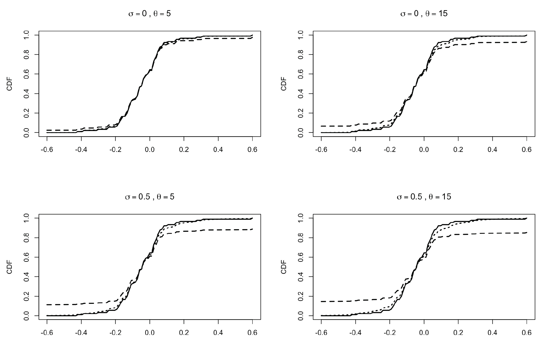
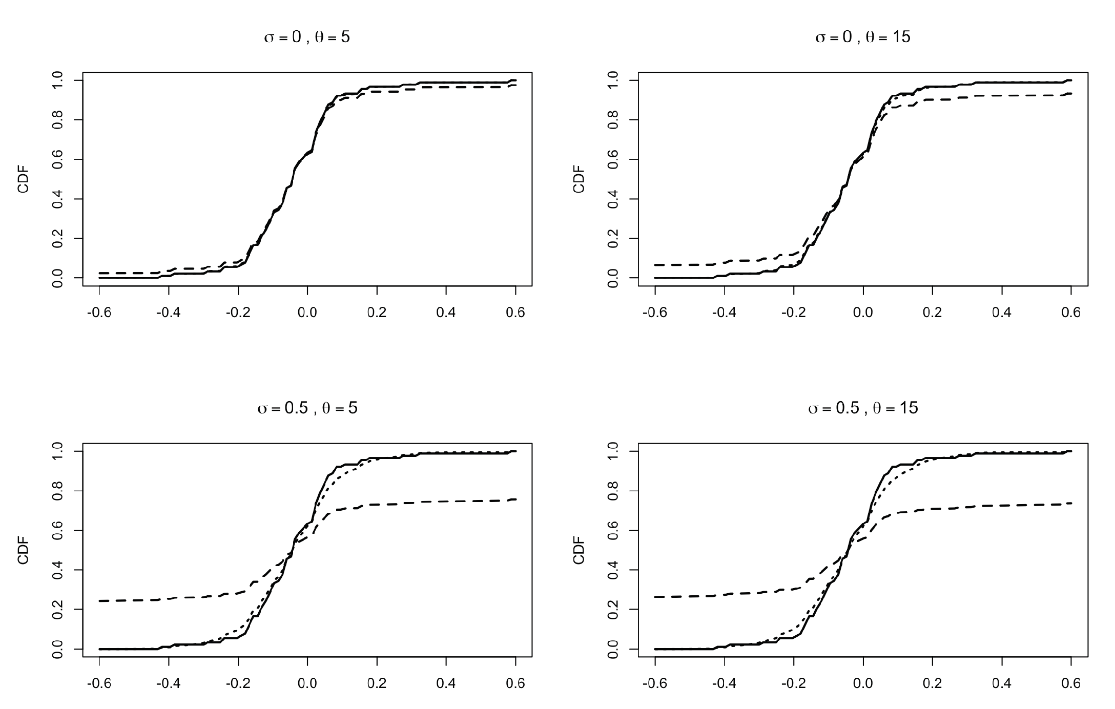
We show an application of (33) to a true dataset by choosing and according to a Pitman–Yor two-parameter family; see (23). The data are the relative changes in reported larcenies between 1991 and 1995 (relative to 1991) for the 90 most populous US counties, taken from Section 2.1 of [34]. We apply our models to both the raw data and the rounded data (approximated to the second digit) in order to obtain ties in the ξs. In the evaluation of the predictive CDFs, we fix , , and . In Figure 2, we report the empirical CDF of the rounded data (solid line), the predictive CDF obtained from (33) (dotted line) and the predictive CDF of a Pitman–Yor species sampling sequence (see PS2) with , (dashed line). Similar plots are reported in Figure 3, with raw data in place of the rounded data. Note that in all the various settings, the influence of the hyper-parameters is stronger in the CDF of the simple Pitman–Yor species sampling model with respect to the corresponding predictive CDF derived from (33).
5.2. Predictive Distributions for
We now deduce an explicit form for the predictive distribution of a with general base measure H given in (25).
Recall that we denote by the partition induced by , with , and by the latent partition appearing in Proposition 3. We also set
The variable is a discrete random variable that takes value 0 if comes from the diffuse component of H.
Let be the set of all the possible configurations of that are compatible with the observed partition and the additional information given by , . In order to describe this set, observe that if , then the block may arise from the union of more blocks in , while, if , then for some . Note that it may happen that .
Recalling that the elements in in (17) are used to describe the numbers of sub-blocks into which the blocks of have been divided to form the latent partition , it turns out that the set has the additional constraint whenever . These considerations yield that, starting from and , the set of admissible can also be described by resorting to the definition of as follows:
With this position, one has
where and have been defined in Section 4.1.
For any in and any in , we define
In other words, corresponds to the configuration obtained from by adding one new element as a new block. In the following, let , and let be obtained from by adding 1 to its i-th component.
Proposition 8.
Let be a . Then, for any A in ,
where
Proof.
We start by defining the following events for :
Since conditioning on is equivalent to the condition on , one can write
Now, set
and
On , one has (up to zero probability sets)
while, on (up to zero probability sets),
Note that (up to zero probability sets)
Hence,
Similarly, using that , one obtains
where
At this stage, note that, by construction,
where is characterized by
and then
Hence,
which shows, in particular, that and are conditionally independent given . Since , and depend logically only on , one obtains
and, finally,
Since are discrete random variables, we use the elementary definition of the conditional probability of events to evaluate the conditional distributions (38) and (39). Specifically, assume that , , , and, for a given event E, write
As for the denominator in (40), letting and , using (34), one obtains
As for the numerators in (40), when , we start from
where, in the last equality, we used that for , one has
Taking the sum over gives
Combining these with (39) and (40) and recalling that , one obtains
Finally, it remains to consider (40) when . Now, observe that
where denote the partition in obtained from by adding to the i-th block of . Note that, for the second equality, we used that, on , one has .
Combining these results, one obtains the thesis. □
6. Conclusions and Discussion
We have defined a new class of exchangeable sequences, called mixtures of species sampling sequences (mSSS). We have shown that these sequences include various well-known Bayesian nonparametric models. In particular, the observations of many nonparametric hierarchical models (e.g., hierarchical Dirichlet process, hierarchical Pitman–Yor process and, more generally, hierarchical species sampling models [22,23,24,25]) are mSSS. We have shown that also observations sampled from a mixture of Dirichlet processes [10] are mSSS, under some additional assumptions. Our general class also includes species sampling sequences with a general (not necessarily diffuse) base measure, which have been used in various applications, e.g., in the case of “spike-and-slab”-type nonparametric priors [16,17,18,19,20,21].
We believe that our general framework sheds light on the common structure of all the above-mentioned models, leading to a possible unified treatment of some of their important features. Our techniques provides unified proofs for various results that, up to now, have been proven with ad hoc methods.
We have proven that all the mSSS are obtained by assigning the values of an exchangeable sequence to the classes of a latent exchangeable random partition. This representation is proven in the strong sense of an almost sure equality (see Section 3) and leads to the simple and clear derivation of an explicit expression for the EPPF of an mSSS. We believe that our general proof simplifies the derivation of the EPPF of many of the above-mentioned particular cases. Moreover, our results show that the clustering and the predictive structure of various well-known models do not depend on the relation between these models and completely random measures, but are essentially a consequence of the simple combinatorial structure of these sequences. Many important differences between well-known models (such as mixtures of Dirichlet and hierarchical Dirichlet) can be explained easily by simple differences in the latent partition and the corresponding latent exchangeable sequence.
We stress that a clear understanding of the clustering structure of mSSS is fundamental for practical purposes, since these models are typically used to cluster observations. Moreover, we hope that the explicit expression for EPPFs in our general framework can lead to the development of new MCMC algorithms for sampling from the posterior distribution.
Finally, we believe that some of the results we have proven here for mSSS can be extended to the more general case of partially exchangeable arrays. In this direction, for future works, a possible generalization of mSSS is to consider partially exchangeable arrays with a mixture of species sampling random probability measures as directing measures.
Author Contributions
F.B.: Methodology, simulation, writing and editing. L.L.: Methodology, writing and editing. All authors have read and agreed to the published version of the manuscript.
Funding
This research received funding from the European Research Council (ERC) under the European Union’s Horizon 2020 research and innovation programme under grant agreement No. 817257.
Institutional Review Board Statement
Not applicable.
Informed Consent Statement
Not applicable.
Data Availability Statement
Not applicable.
Acknowledgments
F. Bassetti and L. Ladelli wish to express their gratitude to Professor Eugenio Regazzini, who has been an inspiring teacher and outstanding guide in many fields of probability and statistics.
Conflicts of Interest
The authors declare no conflict of interest.
Appendix A
In what follows, denotes the law of a random element X. For ease of reference, we state here Lemma 5.9 and Corollary 5.11 of [35].
Lemma A1
(Extension 1). Fix a probability kernel K between two measurable spaces S and T, and let σ be a random element defined on taking values in S. Then, there exists a random element η in T, defined on some extension of the original probability space Ω, such that a.s. and, moreover, η is conditionally independent given σ from any other random element on Ω.
Lemma A2
(Extension 2). Fix two Borel spaces S and T, a measurable mapping and some random elements σ in S and in T with . Then, there is a random element η defined on some extension of the original probability space, such that and a.s.
We need the following variant of the previous result.
Lemma A3
(Extension 3). Fix three Borel spaces , and , a measurable mapping and some random elements in and in , all defined on a probability space . Assume that the conditional law of given is the same as the conditional law of given (P-almost surely). Then, there is a random element τ defined on some extension of the original probability space taking values in such that
- a.s.
- .
Proof.
Define by , set and . By hypothesizing, it is clear that . Thus, by Lemma A2, one has that, on an enlargement of , there exists such that and a.s. Hence, a.s. but also a.s. It remains to show the second part of the thesis. Since a.s. and , where , it follows that . □
References
- Ferguson, T.S. A Bayesian analysis of some nonparametric problems. Ann. Stat. 1973, 1, 209–230. [Google Scholar] [CrossRef]
- Pitman, J.; Yor, M. The two-parameter Poisson-Dirichlet distribution derived from a stable subordinator. Ann. Probab. 1997, 25, 855–900. [Google Scholar] [CrossRef]
- Perman, M.; Pitman, J.; Yor, M. Size-biased sampling of Poisson point processes and excursions. Probab. Theory Relat. Fields 1992, 92, 21–39. [Google Scholar] [CrossRef]
- Regazzini, E.; Lijoi, A.; Prünster, I. Distributional results for means of normalized random measures with independent increments. Ann. Stat. 2003, 31, 560–585. [Google Scholar] [CrossRef]
- James, L.F.; Lijoi, A.; Prünster, I. Posterior analysis for normalized random measures with independent increments. Scand. J. Stat. 2009, 36, 76–97. [Google Scholar] [CrossRef]
- Lijoi, A.; Prünster, I. Models beyond the Dirichlet process. In Bayesian Nonparametrics; Hjort, N.L., Holmes, C., Müller, P., Walker, S., Eds.; Cambridge University Press: New York, NY, USA, 2010. [Google Scholar]
- De Blasi, P.; Favaro, S.; Lijoi, A.; Mena, R.H.; Prunster, I.; Ruggiero, M. Are Gibbs-Type Priors the Most Natural Generalization of the Dirichlet Process? IEEE Trans. Pattern Anal. Mach. Intell. 2015, 37, 212–229. [Google Scholar] [CrossRef] [Green Version]
- Pitman, J. Poisson-Kingman partitions. In Statistics and Science: A Festschrift for Terry Speed; IMS Lecture Notes Monograph Series; Institute of Mathematical Statistics: Beachwood, OH, USA, 2003; Volume 40, pp. 1–34. [Google Scholar]
- Ishwaran, H.; James, L.F. Gibbs sampling methods for stick-breaking priors. J. Am. Stat. Assoc. 2001, 96, 161–173. [Google Scholar] [CrossRef]
- Antoniak, C.E. Mixtures of Dirichlet processes with applications to Bayesian nonparametric problems. Ann. Stat. 1974, 2, 1152–1174. [Google Scholar] [CrossRef]
- Cifarelli, D.M.; Regazzini, E. Distribution functions of means of a Dirichlet process. Ann. Stat. 1990, 18, 429–442. [Google Scholar] [CrossRef]
- Sangalli, L.M. Some developments of the normalized random measures with independent increments. Sankhyā 2006, 68, 461–487. [Google Scholar]
- Broderick, T.; Wilson, A.C.; Jordan, M.I. Posteriors, conjugacy, and exponential families for completely random measures. Bernoulli 2018, 24, 3181–3221. [Google Scholar] [CrossRef] [Green Version]
- Bassetti, F.; Ladelli, L. Asymptotic number of clusters for species sampling sequences with non-diffuse base measure. Stat. Probab. Lett. 2020, 162, 108749. [Google Scholar] [CrossRef]
- Pitman, J. Some developments of the Blackwell-MacQueen urn scheme. In Statistics, Probability and Game Theory; IMS Lecture Notes Monograph Series; Institute of Mathematical Statistics: Hayward, CA, USA, 1996; Volume 30, pp. 245–267. [Google Scholar] [CrossRef]
- Dunson, D.B.; Herring, A.H.; Engel, S.M. Bayesian selection and clustering of polymorphisms in functionally related genes. J. Am. Stat. Assoc. 2008, 103, 534–546. [Google Scholar] [CrossRef]
- Kim, S.; Dahl, D.B.; Vannucci, M. Spiked Dirichlet process prior for Bayesian multiple hypothesis testing in random effects models. Bayesian Anal. 2009, 4, 707–732. [Google Scholar] [CrossRef] [PubMed]
- Suarez, A.J.; Ghosal, S. Bayesian Clustering of Functional Data Using Local Features. Bayesian Anal. 2016, 11, 71–98. [Google Scholar] [CrossRef]
- Cui, K.; Cui, W. Spike-and-Slab Dirichlet Process Mixture Models. Spike Slab Dirichlet Process. Mix. Model. 2012, 2, 512–518. [Google Scholar] [CrossRef] [Green Version]
- Barcella, W.; De Iorio, M.; Baioa, G.; Malone-Leeb, J. Variable selection in covariate dependent random partition models: An application to urinary tract infection. Stat. Med. 2016, 35, 1373–13892. [Google Scholar] [CrossRef] [Green Version]
- Canale, A.; Lijoi, A.; Nipoti, B.; Prünster, I. On the Pitman–Yor process with spike and slab base measure. Biometrika 2017, 104, 681–697. [Google Scholar] [CrossRef]
- Teh, Y.; Jordan, M.I. Hierarchical Bayesian nonparametric models with applications. In Bayesian Nonparametrics; Hjort, N.L., Holmes, C., Müller, P., Walker, S., Eds.; Cambridge University Press: New York, NY, USA, 2010. [Google Scholar]
- Teh, Y.W.; Jordan, M.I.; Beal, M.J.; Blei, D.M. Hierarchical Dirichlet processes. J. Am. Stat. Assoc. 2006, 101, 1566–1581. [Google Scholar] [CrossRef]
- Camerlenghi, F.; Lijoi, A.; Orbanz, P.; Pruenster, I. Distribution theory for hierarchical processes. Ann. Stat. 2019, 1, 67–92. [Google Scholar] [CrossRef] [Green Version]
- Bassetti, F.; Casarin, R.; Rossini, L. Hierarchical Species Sampling Models. Bayesian Anal. 2020, 15, 809–838. [Google Scholar] [CrossRef]
- Pitman, J. Combinatorial Stochastic Processes; Lectures from the 32nd Summer School on Probability Theory Held in Saint-Flour, 7–24 July 2002, with a Foreword by Jean Picard; Lecture Notes in Mathematics; Springer: Berlin, Germany, 2006; Volume 1875. [Google Scholar]
- Crane, H. The ubiquitous Ewens sampling formula. Stat. Sci. 2016, 31, 1–19. [Google Scholar] [CrossRef]
- Kingman, J.F.C. The representation of partition structures. J. Lond. Math. Soc. 1978, 18, 374–380. [Google Scholar] [CrossRef]
- Aldous, D.J. Exchangeability and related topics. In École d’été de Probabilités de Saint-Flour, XIII—1983; Lecture Notes in Mathematics; Springer: Berlin, Germany, 1985; Volume 1117, pp. 1–198. [Google Scholar] [CrossRef]
- Kallenberg, O. Canonical representations and convergence criteria for processes with interchangeable increments. Z. Wahrscheinlichkeitstheorie Und Verw. Geb. 1973, 27, 23–36. [Google Scholar] [CrossRef]
- Pitman, J. Exchangeable and partially exchangeable random partitions. Probab. Theory Relat. Fields 1995, 102, 145–158. [Google Scholar] [CrossRef]
- Gnedin, A.; Pitman, J. Exchangeable Gibbs partitions and Stirling triangles. Zap. Nauchn. Sem. S.-Peterburg. Otdel. Mat. Inst. Steklov. (POMI) 2005, 325, 83–102, 244–245. [Google Scholar] [CrossRef] [Green Version]
- Schervish, M.J. Theory of Statistics; Springer Series in Statistics; Springer: New York, NY, USA, 1995. [Google Scholar] [CrossRef]
- Marin, J.M.; Robert, C.P. Bayesian Core: A Practical Approach to Computational Bayesian Statistics; Springer Texts in Statistics; Springer: New York, NY, USA, 2007; pp. xiv+255. [Google Scholar]
- Kallenberg, O. Foundations of Modern Probability, 3rd ed.; Probability Theory and Stochastic Modelling; Springer: New York, NY, USA, 2021; Volume 99. [Google Scholar]
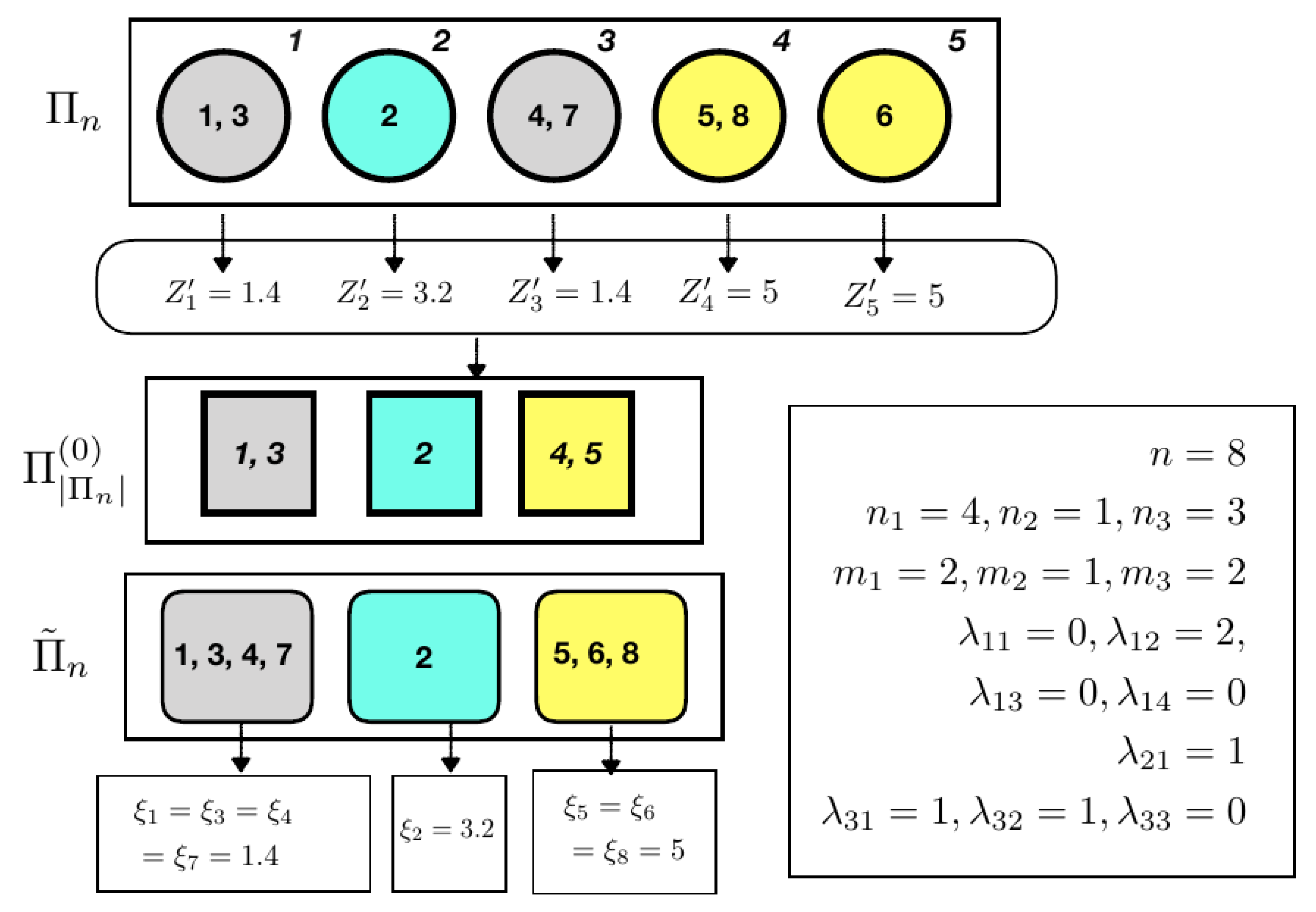
Figure 1.
Pictorial representation of the latent partition structure of an mSSS. In the example, the partition induced by for is , and it is represented using rounded squares (left bottom). Circles at the top left represent a compatible latent partition, namely . The partition on induced by the latent , i.e., , is represented with squares in the middle of the figure. Combining and , one obtains . The statistics , and corresponding to this particular configuration are shown in the box at the bottom right.

Figure 2.
Predictive CDFs for the relative changes in larcenies between 1991 and 1995 (relative to 1991) for the 90 most populous US counties; data taken from Section 2.1 of [34]. Data have been rounded to the second decimal. Here, and . Solid line: empirical CDF. Dotted line: predictive CDF from (33). Dashed line: predictive CDF from PS2 with , . Different plots correspond to different values of and . In all the plots, the predictive CDFs are evaluated with , , and .

Figure 3.
Predictive CDFs for the relative changes in larcenies between 1991 and 1995 (relative to 1991) for the 90 most populous US counties; data taken from Section 2.1 of [34]. Raw data, without rounding. Here, and . Solid line: empirical CDF. Dotted line: predictive CDF from (33). Dashed line: predictive CDF from PS2 with , . Different plots correspond to different values of and . In all the plots, the predictive CDFs are evaluated with , , and .

Publisher’s Note: MDPI stays neutral with regard to jurisdictional claims in published maps and institutional affiliations. |
© 2021 by the authors. Licensee MDPI, Basel, Switzerland. This article is an open access article distributed under the terms and conditions of the Creative Commons Attribution (CC BY) license (https://creativecommons.org/licenses/by/4.0/).
Share and Cite
MDPI and ACS Style
Bassetti, F.; Ladelli, L. Mixture of Species Sampling Models. Mathematics 2021, 9, 3127. https://doi.org/10.3390/math9233127
AMA Style
Bassetti F, Ladelli L. Mixture of Species Sampling Models. Mathematics. 2021; 9(23):3127. https://doi.org/10.3390/math9233127
Chicago/Turabian StyleBassetti, Federico, and Lucia Ladelli. 2021. "Mixture of Species Sampling Models" Mathematics 9, no. 23: 3127. https://doi.org/10.3390/math9233127
Note that from the first issue of 2016, this journal uses article numbers instead of page numbers. See further details here.