Resolutions of the Jerk and Snap Vectors for a Quasi Curve in Euclidean 3-Space

Abstract

This work aims at studying resolutions of the jerk and snap vectors of a point particle moving along a quasi curve in Euclidean 3-space ${\mathbb{E}}^3$. In particular, we obtain the resolution of the jerk and snap vectors along the quasi vectors and offer an alternative resolution of the jerk and snap vectors along the tangential direction and two special radial directions that lie in the osculating and rectifying planes. This alternative resolution for a quasi plane curve in Euclidean 3-space ${\mathbb{E}}^3$ is given as corollary. Moreover, our results are illustrated via some examples.

1. Introduction

There is a very close relationship between the kinematics of a moving particle and the differential geometry of the trajectory where any point particle of constant mass moving along a trajectory in the space has a position vector according to the moving frame for the trajectory. Displacement, velocity, and acceleration are all terms that we are all familiar with. We experience velocity when we move and acceleration when we change the velocity at which we move. When acceleration is rapidly changing, we feel jerk and snap. The terms jerk and snap mean very little to most people. Mathematically, the velocity, acceleration, jerk (jolt), and snap (jounce) are the first, second, third, and fourth derivatives of the position with respect to time, respectively. We can observe the effects of velocity, acceleration, and higher-order derivatives when driving a car. A more experienced driver accelerates smoothly, whereas a novice driver may produce a jerky ride, causing jerk and snap.

Jerk and snap can be observed in many areas. In physics and engineering, when transition and vibration occur, especially when this excitation causes multi-resonant modes of vibration. In mechanical engineering, when the cam-follower jumps off the camshaft in the automotive sense. In civil engineering, when switching between train tracks and roads suddenly. Jerk and snap have many applications in oscillators, manufacturing and motion control, see [1,2,3].

A curve provided with the Frenet, Darboux, modified, Bishop, or quasi frame is called the Frenet, Darboux, modified, Bishop, or quasi curve, respectively. In most applications, the acceleration is expressed as the sum of its normal and tangential components. Siacci [4] obtained the acceleration vector as the sum of its radial and tangential components. Despite Siacci’s theorem being very remarkable, his formulation of the theorem is inaccurate and his proof is burdensome. Therefore, Whittaker [5] and Grossman [6] presented a more modern geometrical proof of Siacci’s theorem in the plane. Casey [7] presented a proof of Siacci’s theorem for Frenet curves in Euclidean 3-space ${\mathbb{E}}^3$. Küçükarslan et al. [8] studied Siacci’s theorem for curves in Finsler Manifold ${\mathbb{F}}^3$. Özen et al. [9] studied Siacci’s theorem for Darboux curves on regular surfaces in Euclidean 3-space ${\mathbb{E}}^3$. Özen [10] studied Siacci’s theorem for Frenet curves in Minkowski 3-space ${\mathbb{E}}_1^3$. Résal [11] obtained a resolution of the jerk vector for Frenet curves in Euclidean 3-space ${\mathbb{E}}^3$. Özen et al. [12] presented a new resolution of the jerk vector for Frenet curves in Euclidean 3-space ${\mathbb{E}}^3$. Özen et al. [13] studied resolutions of the acceleration and jerk vectors for modified curves in Euclidean 3-space ${\mathbb{E}}^3$. Güner [14] studied resolutions of the jerk vector for Bishop curves in Euclidean 3-space ${\mathbb{E}}^3$. Tosun and Hızarcıoglu [15] studied resolutions of the jerk vector for Darboux curves on regular surfaces in Euclidean 3-space ${\mathbb{E}}^3$. For more details about the jerk and snap vectors, see [1,16,17].

The moving frames play an essential role in studying curves and surfaces in different spaces, especially the quasi frame, which is more efficient and general than other frames (Frenet, Bishop). This frame characterized as well-defined at all points, its calculations are easy and its construction does not change if the curve parameterized by arc-length or not.

The purpose of this work is to study resolutions of the jerk and snap vectors of a point particle moving along a quasi curve in Euclidean 3-space ${\mathbb{E}}^3$. This article is organized as follows: In Section 2, we present background about the quasi frame along a unit speed curve in Euclidean 3-space ${\mathbb{E}}^3$ and its relation to the Frenet frame. In Section 3, we obtain the resolution of the jerk and snap vectors of a point particle according to the quasi frame and provide an alternative resolution of the jerk and snap vectors along the tangential direction and two special radial directions. Moreover, the tangential and special radial components of the jerk and snap vectors for a quasi plane curve in Euclidean 3-space ${\mathbb{E}}^3$ are given as a corollary. 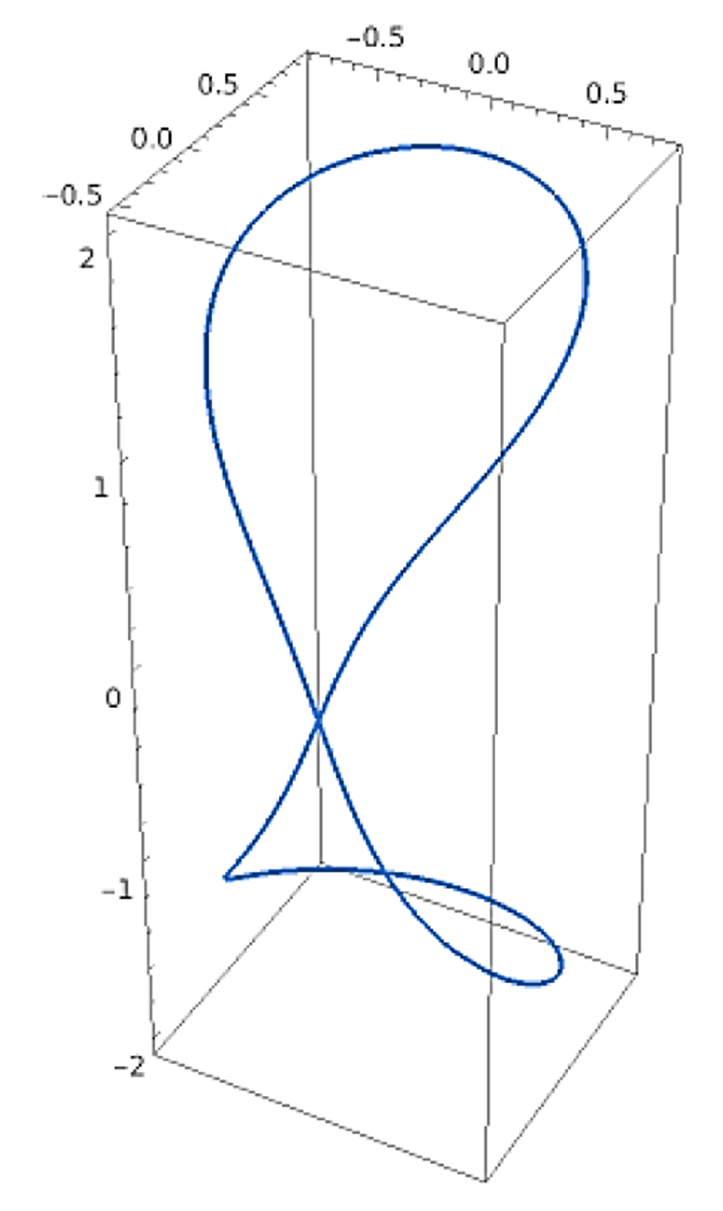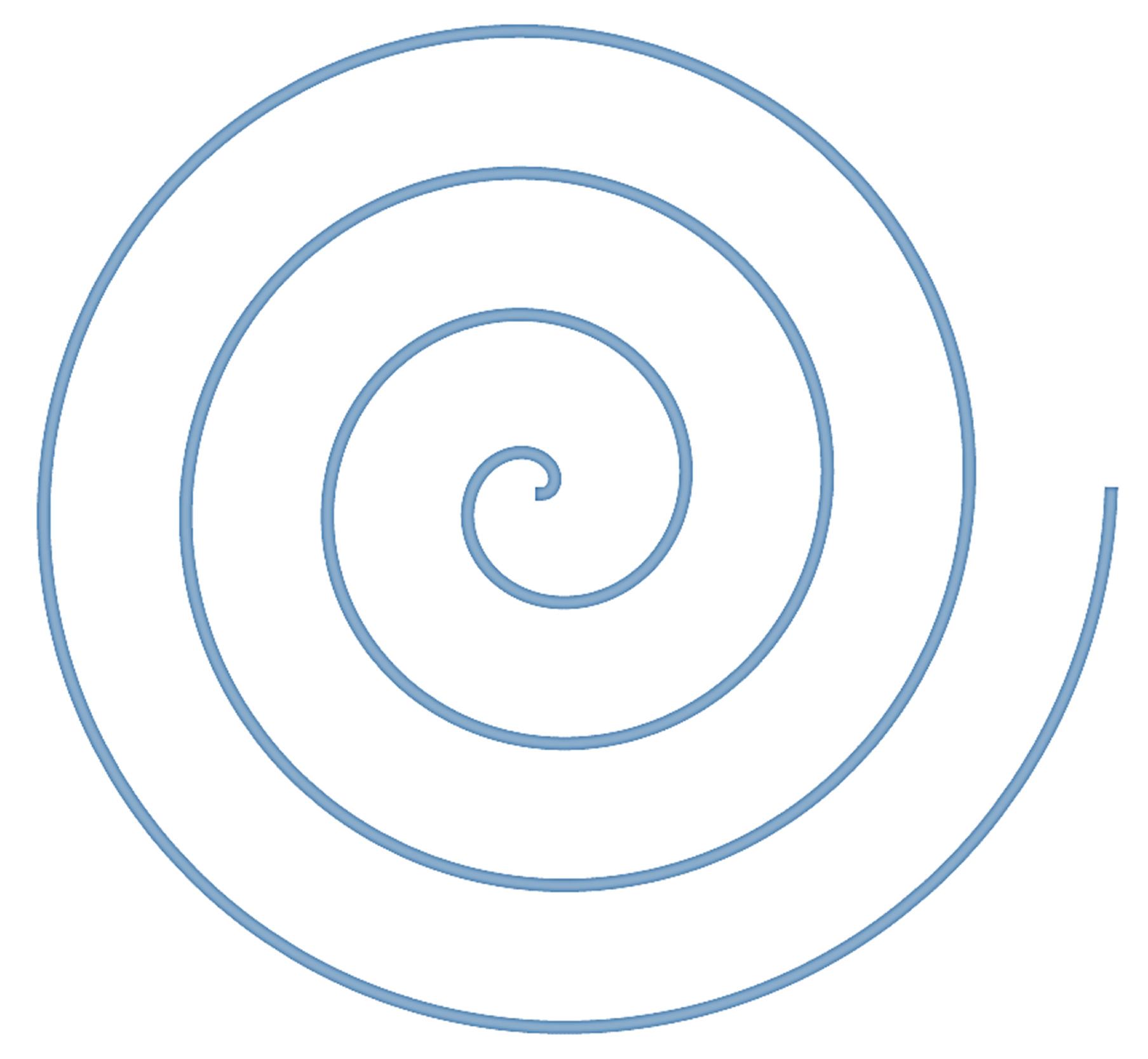In Section 4, we offer illustrative examples to show our results. Finally, in Section 5, we conclude the article with a summary.

2. Preliminaries

In this section, we start with the basic concepts of this paper.

Let ${\mathbb{E}}^3$ be a Euclidean 3-space provided with the Cartesian metric g given by

$$g=d{x}_1^2+d{x}_2^2+d{x}_3^2,$$

where $\left(x_1,x_2,x_3\right)$ is a coordinate system of ${\mathbb{E}}^3$. Let $P=\left(p_1,p_2,p_3\right)$ and $Q=\left(q_1,q_2,q_3\right)$ be any two vectors in ${\mathbb{E}}^3$. Then, we can define the following:

-

The Cartesian inner product of P and Q as

$$〈P,Q〉=p_1{q}_1+p_2{q}_2+p_3{q}_3;$$

-

The Cartesian norm of Q by

$$∥Q∥=\sqrt{〈Q,Q〉};$$

-

The Cartesian cross product of P and Q as

$$P\times Q=\left|\begin{array}{ccc}{e}_1& e_2& e_3\\ p_1& p_2& p_3\\ q_1& q_2& q_3\end{array}\right|=\left(p_2{q}_3-p_3{q}_2,p_3{q}_1-p_1{q}_3,p_1{q}_2-p_2{q}_1\right).$$

Definition 1.

A differentiable curve $\alpha \left(s\right)$ in ${\mathbb{E}}^3$ is termed a regular curve if ${\alpha }^{\prime }\left(s\right)\ne 0$ for each s, while it is termed a unit speed curve or an arc-length parameterized curve if $∥{\alpha }^{\prime }\left(s\right)∥=1$ for each s.

Let $\alpha \left(s\right)$ be a unit speed curve in ${\mathbb{E}}^3$ such that ${\alpha }^{\prime \prime }\left(s\right)\ne 0$ for all s. Then, we can define the following [18,19,20]:

-

The Frenet orthonormal frame $\left\{\mathbf{T}\left(s\right),\mathbf{N}\left(s\right),\mathbf{B}\left(s\right)\right\}$ along the curve $\alpha \left(s\right)$ as

$$\mathbf{T}\left(s\right)={\alpha }^{\prime }\left(s\right),\mathbf{N}\left(s\right)=\frac{{\mathbf{T}}^{\prime }\left(s\right)}{∥{\mathbf{T}}^{\prime }\left(s\right)∥},\mathbf{B}\left(s\right)=\mathbf{T}\left(s\right)\times \mathbf{N}\left(s\right),$$

(1)

where $\mathbf{T}\left(s\right)$, $\mathbf{N}\left(s\right)$ and $\mathbf{B}\left(s\right)$ are the unit tangent, Frenet-normal and Frenet-binormal vectors, respectively. Therefore, the Frenet equations for the curve $\alpha \left(s\right)$ are given by

$$\left[\begin{array}{c}{\mathbf{T}}^{\prime }\left(s\right)\\ {\mathbf{N}}^{\prime }\left(s\right)\\ {\mathbf{B}}^{\prime }\left(s\right)\end{array}\right]=\left[\begin{array}{ccc}0& \kappa & 0\\ -\kappa & 0& \tau \\ 0& -\tau & 0\end{array}\right]\left[\begin{array}{c}\mathbf{T}\left(s\right)\\ \mathbf{N}\left(s\right)\\ \mathbf{B}\left(s\right)\end{array}\right],$$

(2)

where the functions $\kappa$ and $\tau$ are Frenet-curvatures for the curve $\alpha \left(s\right)$ and defined by

$$\kappa \left(s\right)=∥{\mathbf{T}}^{\prime }\left(s\right)∥,\tau \left(s\right)=-〈{\mathbf{B}}^{\prime }\left(s\right),\mathbf{N}\left(s\right)〉.$$

(3)

-

The quasi orthonormal frame $\left\{\mathbf{T}\left(s\right),{\mathbf{N}}_{\mathbf{q}}\left(s\right),{\mathbf{B}}_{\mathbf{q}}\left(s\right)\right\}$ along the curve $\alpha \left(s\right)$ as

$$\mathbf{T}\left(s\right)={\alpha }^{\prime }\left(s\right),{\mathbf{N}}_{\mathbf{q}}\left(s\right)=\frac{\mathbf{T}\times \mathbf{k}}{∥\mathbf{T}\times \mathbf{k}∥},{\mathbf{B}}_{\mathbf{q}}\left(s\right)=\mathbf{T}\times {\mathbf{N}}_{\mathbf{q}},$$

(4)

where $\mathbf{T}\left(s\right)$, ${\mathbf{N}}_{\mathbf{q}}\left(s\right)$,${\mathbf{B}}_{\mathbf{q}}\left(s\right)$ and $\mathbf{k}$ are the unit tangent, quasi-normal, quasi-binormal and projection vectors, respectively. The projection vector equals $\left(1,0,0\right)$ or $\left(0,1,0\right)$ or $\left(0,0,1\right)$.

-

The relation matrix between the quasi frame and Frenet frame along the curve $\alpha \left(s\right)$ by

$$\left[\begin{array}{c}\mathbf{T}\left(s\right)\\ {\mathbf{N}}_{\mathbf{q}}\left(s\right)\\ {\mathbf{B}}_{\mathbf{q}}\left(s\right)\end{array}\right]=\left[\begin{array}{ccc}1& 0& 0\\ 0& cos\varphi & sin\varphi \\ 0& -sin\varphi & cos\varphi \end{array}\right]\left[\begin{array}{c}\mathbf{T}\left(s\right)\\ \mathbf{N}\left(s\right)\\ \mathbf{B}\left(s\right)\end{array}\right].$$

(5)

Thus, we have

$$\left[\begin{array}{c}\mathbf{T}\left(s\right)\\ \mathbf{N}\left(s\right)\\ \mathbf{B}\left(s\right)\end{array}\right]=\left[\begin{array}{ccc}1& 0& 0\\ 0& cos\varphi & -sin\varphi \\ 0& sin\varphi & cos\varphi \end{array}\right]\left[\begin{array}{c}\mathbf{T}\left(s\right)\\ {\mathbf{N}}_{\mathbf{q}}\left(s\right)\\ {\mathbf{B}}_{\mathbf{q}}\left(s\right)\end{array}\right],$$

(6)

where $\varphi \left(s\right)$ is the Cartesian angle between the Frenet-normal $\mathbf{N}\left(s\right)$ and quasi-normal ${\mathbf{N}}_{\mathbf{q}}\left(s\right)$. By using (2), (5) and (6), the quasi equations for the curve $\alpha \left(s\right)$ are given by

$$\left[\begin{array}{c}{\mathbf{T}}^{\prime }\left(s\right)\\ {\mathbf{N}}_{\mathbf{q}}^{\prime }\left(s\right)\\ {\mathbf{B}}_{\mathbf{q}}^{\prime }\left(s\right)\end{array}\right]=\left[\begin{array}{ccc}0& {\kappa }_1& {\kappa }_2\\ -{\kappa }_1& 0& {\kappa }_3\\ -{\kappa }_2& -{\kappa }_3& 0\end{array}\right]\left[\begin{array}{c}\mathbf{T}\left(s\right)\\ {\mathbf{N}}_{\mathbf{q}}\left(s\right)\\ {\mathbf{B}}_{\mathbf{q}}\left(s\right)\end{array}\right],$$

(7)

where the functions $\left\{{\kappa }_i\left|i=1,2,3\right.\right\}$ are quasi-curvatures for the curve $\alpha \left(s\right)$ and defined by

$${\kappa }_1=\kappa cos\varphi \left(s\right),{\kappa }_2=-\kappa sin\varphi \left(s\right),{\kappa }_3={\varphi }^{\prime }\left(s\right)+\tau .$$

(8)

Thus, we have

$${\kappa }^2={\kappa }_1^2+{\kappa }_2^2,\varphi \left(s\right)=-arctan\left(\frac{{\kappa }_2}{{\kappa }_1}\right).$$

(9)

Remark 1.

The quasi frame is singular if the vectors $\mathbf{T}$ and $\mathbf{k}$ are linearly dependent.

Remark 2.

If we put ${\kappa }_2=0$ in (7), then the quasi equations reduce to the Frenet equations.

During the following sections of our paper, we shall need the following definitions and notation.

Definition 2.

The first, second, third, and fourth time derivatives of the position vector are termed the velocity, acceleration, jerk (jolt), and snap (jounce) vectors, respectively.

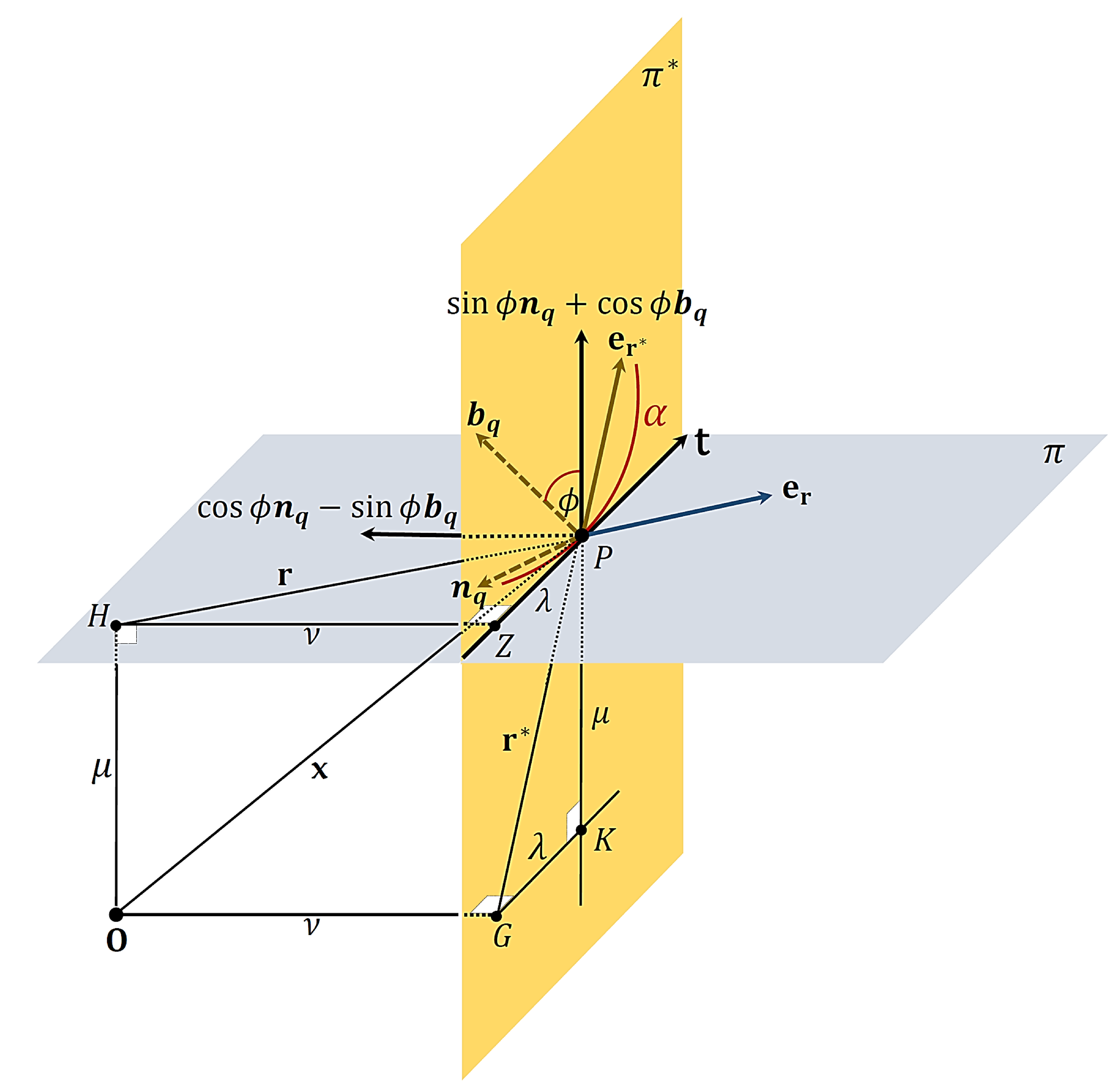
Notation 1.

The osculating and rectifying planes are denoted by π and ${\pi }^{*}$, respectively. The radial directions in the planes π and ${\pi }^{*}$ are denoted by $H\mathcal{P}$ and $G\mathcal{P}$, respectively. The foots of perpendicular lines that are from a fixed origin $\mathcal{O}$ to the planes π and ${\pi }^{*}$ are denoted by H and G, respectively. The unit vectors in directions $H\mathcal{P}$ and $G\mathcal{P}$ are denoted by ${\mathbf{e}}_{\mathbf{r}}$ and ${\mathbf{e}}_{{\mathbf{r}}^{*}}$, respectively. The angular momentum vector of a point particle $\mathcal{P}$ about a fixed origin $\mathcal{O}$ is denoted by ${\mathcal{H}}^{\mathcal{O}}$.

3. Main Results

In this section, we obtain the resolution of the jerk and snap vectors of a point particle along a quasi curve and provide an alternative resolution of the jerk and snap vectors along the tangential direction and two special radial directions that lie in the planes $\pi$ and ${\pi }^{*}$.

Theorem 1.

Assume that the point particle $\mathcal{P}$ with constant mass m moves along an arc-length parameterized quasi curve $\alpha \left(s\right)$ in ${\mathbb{E}}^3$. Suppose that the arc-length s of the curve α coincides with time t. Then, we can state the following:

-

The jerk vector of the point particle $\mathcal{P}$ at time t is given as

$$\mathcal{J}={\mathcal{D}}_{\mathbf{t}}\mathbf{T}+{\mathcal{D}}_{{\mathbf{n}}_{\mathbf{q}}}{\mathbf{N}}_{\mathbf{q}}+{\mathcal{D}}_{{\mathbf{b}}_{\mathbf{q}}}{\mathbf{B}}_{\mathbf{q}},$$

(10)

where

$$\begin{array}{ccc}\hfill {\mathcal{D}}_{\mathbf{t}}& =& \left(\frac{{\mathrm{d}}^{3}s}{\mathrm{d}{t}^3}\right)-\left({\kappa }_1^2+{\kappa }_2^2\right){\left(\frac{\mathrm{d}s}{\mathrm{d}t}\right)}^3,\hfill \\ \hfill {\mathcal{D}}_{{\mathbf{n}}_{\mathbf{q}}}& =& \left[3\sqrt{{\kappa }_1^2+{\kappa }_2^2}\left(\frac{\mathrm{d}s}{\mathrm{d}t}\right)\left(\frac{{\mathrm{d}}^{2}s}{\mathrm{d}{t}^2}\right)+{\left(\frac{\mathrm{d}s}{\mathrm{d}t}\right)}^3\frac{\mathrm{d}}{\mathrm{d}s}\left(\sqrt{{\kappa }_1^2+{\kappa }_2^2}\right)\right]cos\varphi \left(s\right)\hfill \\ & & +\left[\left({\kappa }_3-{\varphi }^{\prime }\right)\sqrt{{\kappa }_1^2+{\kappa }_2^2}{\left(\frac{\mathrm{d}s}{\mathrm{d}t}\right)}^3\right]sin\varphi \left(s\right),\hfill \\ \hfill {\mathcal{D}}_{{\mathbf{b}}_{\mathbf{q}}}& =& \left[3\sqrt{{\kappa }_1^2+{\kappa }_2^2}\left(\frac{\mathrm{d}s}{\mathrm{d}t}\right)\left(\frac{{\mathrm{d}}^{2}s}{\mathrm{d}{t}^2}\right)+{\left(\frac{\mathrm{d}s}{\mathrm{d}t}\right)}^3\frac{\mathrm{d}}{\mathrm{d}s}\left(\sqrt{{\kappa }_1^2+{\kappa }_2^2}\right)\right]\left(-sin\varphi \left(s\right)\right)\hfill \\ & & +\left[\left({\kappa }_3-{\varphi }^{\prime }\right)\sqrt{{\kappa }_1^2+{\kappa }_2^2}{\left(\frac{\mathrm{d}s}{\mathrm{d}t}\right)}^3\right]cos\varphi \left(s\right).\hfill \end{array}$$

Here, ${\mathcal{D}}_{\mathbf{t}}$, ${\mathcal{D}}_{{\mathbf{n}}_{\mathbf{q}}}$ and ${\mathcal{D}}_{{\mathbf{b}}_{\mathbf{q}}}$ are the tangential, quasi-normal and quasi-binormal components of the jerk, respectively.

-

The snap vector of the point particle $\mathcal{P}$ at time t is given by

$$\mathcal{S}={\mathcal{C}}_{\mathbf{t}}\mathbf{T}+{\mathcal{C}}_{{\mathbf{n}}_{\mathbf{q}}}{\mathbf{N}}_{\mathbf{q}}+{\mathcal{C}}_{{\mathbf{b}}_{\mathbf{q}}}{\mathbf{B}}_{\mathbf{q}},$$

(11)

where

$$\begin{array}{ccc}\hfill {\mathcal{C}}_{\mathbf{t}}& =& \left(\frac{{\mathrm{d}}^{4}s}{\mathrm{d}{t}^4}\right)-6\left({\kappa }_1^2+{\kappa }_2^2\right){\left(\frac{\mathrm{d}s}{\mathrm{d}t}\right)}^2\left(\frac{{\mathrm{d}}^{2}s}{\mathrm{d}{t}^2}\right)-3\sqrt{{\kappa }_1^2+{\kappa }_2^2}{\left(\frac{\mathrm{d}s}{\mathrm{d}t}\right)}^4\frac{\mathrm{d}}{\mathrm{d}s}\left(\sqrt{{\kappa }_1^2+{\kappa }_2^2}\right),\hfill \\ \hfill {\mathcal{C}}_{{\mathbf{n}}_{\mathbf{q}}}& =& \left[4\sqrt{{\kappa }_1^2+{\kappa }_2^2}\left(\frac{\mathrm{d}s}{\mathrm{d}t}\right)\left(\frac{{\mathrm{d}}^{3}s}{\mathrm{d}{t}^3}\right)+6{\left(\frac{\mathrm{d}s}{\mathrm{d}t}\right)}^2\left(\frac{{\mathrm{d}}^{2}s}{\mathrm{d}{t}^2}\right)\frac{\mathrm{d}}{\mathrm{d}s}\left(\sqrt{{\kappa }_1^2+{\kappa }_2^2}\right)\right.\hfill \\ & & +3\sqrt{{\kappa }_1^2+{\kappa }_2^2}{\left(\frac{{\mathrm{d}}^{2}s}{\mathrm{d}{t}^2}\right)}^2+{\left(\frac{\mathrm{d}s}{\mathrm{d}t}\right)}^4\frac{{\mathrm{d}}^2}{\mathrm{d}{s}^2}\left(\sqrt{{\kappa }_1^2+{\kappa }_2^2}\right)-{\left({\kappa }_1^2+{\kappa }_2^2\right)}^{3/2}{\left(\frac{\mathrm{d}s}{\mathrm{d}t}\right)}^4\hfill \\ & & \left.-{\left({\kappa }_3-{\varphi }^{\prime }\right)}^2\sqrt{{\kappa }_1^2+{\kappa }_2^2}{\left(\frac{\mathrm{d}s}{\mathrm{d}t}\right)}^4\right]cos\varphi \left(s\right)\hfill \\ & & +\left[6\left({\kappa }_3-{\varphi }^{\prime }\right)\sqrt{{\kappa }_1^2+{\kappa }_2^2}{\left(\frac{\mathrm{d}s}{\mathrm{d}t}\right)}^2\left(\frac{{\mathrm{d}}^{2}s}{\mathrm{d}{t}^2}\right)+2\left({\kappa }_3-{\varphi }^{\prime }\right){\left(\frac{\mathrm{d}s}{\mathrm{d}t}\right)}^4\frac{\mathrm{d}}{\mathrm{d}s}\left(\sqrt{{\kappa }_1^2+{\kappa }_2^2}\right)\right.\hfill \\ & & \left.+{\left({\kappa }_3-{\varphi }^{\prime }\right)}^{\prime }\sqrt{{\kappa }_1^2+{\kappa }_2^2}{\left(\frac{\mathrm{d}s}{\mathrm{d}t}\right)}^4\right]sin\varphi \left(s\right),\hfill \\ \hfill {\mathcal{C}}_{{\mathbf{b}}_{\mathbf{q}}}& =& \left[4\sqrt{{\kappa }_1^2+{\kappa }_2^2}\left(\frac{\mathrm{d}s}{\mathrm{d}t}\right)\left(\frac{{\mathrm{d}}^{3}s}{\mathrm{d}{t}^3}\right)+6{\left(\frac{\mathrm{d}s}{\mathrm{d}t}\right)}^2\left(\frac{{\mathrm{d}}^{2}s}{\mathrm{d}{t}^2}\right)\frac{\mathrm{d}}{\mathrm{d}s}\left(\sqrt{{\kappa }_1^2+{\kappa }_2^2}\right)\right.\hfill \\ & & +3\sqrt{{\kappa }_1^2+{\kappa }_2^2}{\left(\frac{{\mathrm{d}}^{2}s}{\mathrm{d}{t}^2}\right)}^2+{\left(\frac{\mathrm{d}s}{\mathrm{d}t}\right)}^4\frac{{\mathrm{d}}^2}{\mathrm{d}{s}^2}\left(\sqrt{{\kappa }_1^2+{\kappa }_2^2}\right)-{\left({\kappa }_1^2+{\kappa }_2^2\right)}^{3/2}{\left(\frac{\mathrm{d}s}{\mathrm{d}t}\right)}^4\hfill \\ & & \left.-{\left({\kappa }_3-{\varphi }^{\prime }\right)}^2\sqrt{{\kappa }_1^2+{\kappa }_2^2}{\left(\frac{\mathrm{d}s}{\mathrm{d}t}\right)}^4\right]\left(-sin\varphi \left(s\right)\right)\hfill \\ & & +\left[6\left({\kappa }_3-{\varphi }^{\prime }\right)\sqrt{{\kappa }_1^2+{\kappa }_2^2}{\left(\frac{\mathrm{d}s}{\mathrm{d}t}\right)}^2\left(\frac{{\mathrm{d}}^{2}s}{\mathrm{d}{t}^2}\right)+2\left({\kappa }_3-{\varphi }^{\prime }\right){\left(\frac{\mathrm{d}s}{\mathrm{d}t}\right)}^4\frac{\mathrm{d}}{\mathrm{d}s}\left(\sqrt{{\kappa }_1^2+{\kappa }_2^2}\right)\right.\hfill \\ & & \left.+{\left({\kappa }_3-{\varphi }^{\prime }\right)}^{\prime }\sqrt{{\kappa }_1^2+{\kappa }_2^2}{\left(\frac{\mathrm{d}s}{\mathrm{d}t}\right)}^4\right]cos\varphi \left(s\right).\hfill \end{array}$$

Here, ${\mathcal{C}}_{\mathbf{t}}$, ${\mathcal{C}}_{{\mathbf{n}}_{\mathbf{q}}}$ and ${\mathcal{C}}_{{\mathbf{b}}_{\mathbf{q}}}$ are the tangential, quasi-normal and quasi-binormal components of the snap, respectively.

Proof. 

Let a point particle $\mathcal{P}$ move along an arc-length parameterized quasi curve $\alpha \left(s\right)$ in the space ${\mathbb{E}}^3$. Then, the point particle has a position vector according to the quasi frame. Let $\mathcal{X}$ be the position vector of $\mathcal{P}$ at time t with respect to a fixed origin $\mathcal{O}$ in the space ${\mathbb{E}}^3$. Through an assumption that “the arc-length of the curve coincides with the time”, the unit tangent vector $\mathbf{T}\left(s\right)$ for the curve $\alpha$ at $\mathcal{P}$ is then given by

$$\mathbf{T}\left(s\right)=\frac{\mathrm{d}\mathcal{X}}{\mathrm{d}s}.$$

(12)

From (7)–(9) and (12), we obtain the velocity $\mathcal{V}$ and acceleration $\mathcal{A}$ vectors of $\mathcal{P}$ at time t according to the quasi frame as

$$\mathcal{V}=\frac{\mathrm{d}\mathcal{X}}{\mathrm{d}t}=\left(\frac{\mathrm{d}s}{\mathrm{d}t}\right)\mathbf{T}$$

(13)

and

$$\mathcal{A}=\left[\frac{{\mathrm{d}}^{2}s}{\mathrm{d}{t}^2}\right]\mathbf{T}+\left[\sqrt{{\kappa }_1^2+{\kappa }_2^2}{\left(\frac{\mathrm{d}s}{\mathrm{d}t}\right)}^{2}cos\varphi \left(s\right)\right]{\mathbf{N}}_{\mathbf{q}}-\left[\sqrt{{\kappa }_1^2+{\kappa }_2^2}{\left(\frac{\mathrm{d}s}{\mathrm{d}t}\right)}^{2}sin\varphi \left(s\right)\right]{\mathbf{B}}_{\mathbf{q}},$$

respectively. From Definition 2, the jerk and snap vectors of the point particle $\mathcal{P}$ according to the quasi frame are expressed as in (10) and (11), respectively. The proof is complete. □

Theorem 2.

Assume that the point particle $\mathcal{P}$ with constant mass m moves along an arc-length parameterized quasi curve $\alpha \left(s\right)$ in ${\mathbb{E}}^3$. Suppose that the components of the vector ${\mathcal{H}}^{\mathcal{O}}$ never vanish. Then, we can state the following:

-

The jerk vector of the point particle $\mathcal{P}$ is given as

$$\mathcal{J}={\mathcal{T}}_{\mathbf{t}}\mathbf{T}+{\mathcal{T}}_{\mathbf{r}}{\mathbf{e}}_{\mathbf{r}}+{\mathcal{T}}_{{\mathbf{r}}^{*}}{\mathbf{e}}_{{\mathbf{r}}^{*},}$$

(14)

where

$$\begin{array}{ccc}\hfill {\mathcal{T}}_{\mathbf{t}}& =& \left(\frac{{\mathrm{d}}^{3}s}{\mathrm{d}{t}^3}\right)-\left({\kappa }_1^2+{\kappa }_2^2\right){\left(\frac{\mathrm{d}s}{\mathrm{d}t}\right)}^3+\frac{3\lambda }{\nu }\sqrt{{\kappa }_1^2+{\kappa }_2^2}\left(\frac{\mathrm{d}s}{\mathrm{d}t}\right)\left(\frac{{\mathrm{d}}^{2}s}{\mathrm{d}{t}^2}\right)\hfill \\ & & +\frac{\lambda }{\nu }{\left(\frac{\mathrm{d}s}{\mathrm{d}t}\right)}^3\frac{\mathrm{d}}{\mathrm{d}s}\left(\sqrt{{\kappa }_1^2+{\kappa }_2^2}\right)-\frac{\lambda \left({\kappa }_3-{\varphi }^{\prime }\right)}{\mu }\sqrt{{\kappa }_1^2+{\kappa }_2^2}{\left(\frac{\mathrm{d}s}{\mathrm{d}t}\right)}^3,\hfill \\ \hfill {\mathcal{T}}_{\mathbf{r}}& =& -\frac{3r}{\nu }\sqrt{{\kappa }_1^2+{\kappa }_2^2}\left(\frac{\mathrm{d}s}{\mathrm{d}t}\right)\left(\frac{{\mathrm{d}}^{2}s}{\mathrm{d}{t}^2}\right)-\frac{r}{\nu }{\left(\frac{\mathrm{d}s}{\mathrm{d}t}\right)}^3\frac{\mathrm{d}}{\mathrm{d}s}\left(\sqrt{{\kappa }_1^2+{\kappa }_2^2}\right),\hfill \\ \hfill {\mathcal{T}}_{{\mathbf{r}}^{*}}& =& \frac{r^{*}\left({\kappa }_3-{\varphi }^{\prime }\right)}{\mu }\sqrt{{\kappa }_1^2+{\kappa }_2^2}{\left(\frac{\mathrm{d}s}{\mathrm{d}t}\right)}^3.\hfill \end{array}$$

Here, ${\mathcal{T}}_{\mathbf{t}}$, ${\mathcal{T}}_{\mathbf{r}}$ and ${\mathcal{T}}_{{\mathbf{r}}^{*}}$ are the tangential and special radial components of the jerk. The special radial components ${\mathcal{T}}_{\mathbf{r}}$ and ${\mathcal{T}}_{{\mathbf{r}}^{*}}$ lie along the lines that pass by the point particle $\mathcal{P}$ and the points H and G, respectively. The tangential component ${\mathcal{T}}_{\mathbf{t}}$ lies along the tangent line $\mathbf{T}$ of the curve α at $\mathcal{P}$.

-

The snap vector of the point particle $\mathcal{P}$ is given by

$$\mathcal{S}={\mathcal{F}}_{\mathbf{t}}\mathbf{T}+{\mathcal{F}}_{\mathbf{r}}{\mathbf{e}}_{\mathbf{r}}+{\mathcal{F}}_{{\mathbf{r}}^{*}}{\mathbf{e}}_{{\mathbf{r}}^{*},}$$

(15)

where

$$\begin{array}{ccc}\hfill {\mathcal{F}}_{\mathbf{t}}& =& \left(\frac{{\mathrm{d}}^{4}s}{\mathrm{d}{t}^4}\right)-6\left({\kappa }_1^2+{\kappa }_2^2\right){\left(\frac{\mathrm{d}s}{\mathrm{d}t}\right)}^2\left(\frac{{\mathrm{d}}^{2}s}{\mathrm{d}{t}^2}\right)-3\sqrt{{\kappa }_1^2+{\kappa }_2^2}{\left(\frac{\mathrm{d}s}{\mathrm{d}t}\right)}^4\frac{\mathrm{d}}{\mathrm{d}s}\left(\sqrt{{\kappa }_1^2+{\kappa }_2^2}\right)\hfill \\ & & +\frac{4\lambda }{\nu }\sqrt{{\kappa }_1^2+{\kappa }_2^2}\left(\frac{\mathrm{d}s}{\mathrm{d}t}\right)\left(\frac{{\mathrm{d}}^{3}s}{\mathrm{d}{t}^3}\right)+\frac{6\lambda }{\nu }{\left(\frac{\mathrm{d}s}{\mathrm{d}t}\right)}^2\left(\frac{{\mathrm{d}}^{2}s}{\mathrm{d}{t}^2}\right)\frac{\mathrm{d}}{\mathrm{d}s}\left(\sqrt{{\kappa }_1^2+{\kappa }_2^2}\right)\hfill \\ & & +\frac{3\lambda }{\nu }\sqrt{{\kappa }_1^2+{\kappa }_2^2}{\left(\frac{{\mathrm{d}}^{2}s}{\mathrm{d}{t}^2}\right)}^2-\frac{6\lambda \left({\kappa }_3-{\varphi }^{\prime }\right)}{\mu }\sqrt{{\kappa }_1^2+{\kappa }_2^2}{\left(\frac{\mathrm{d}s}{\mathrm{d}t}\right)}^2\left(\frac{{\mathrm{d}}^{2}s}{\mathrm{d}{t}^2}\right)\hfill \\ & & +\frac{\lambda }{\nu }{\left(\frac{\mathrm{d}s}{\mathrm{d}t}\right)}^4\frac{{\mathrm{d}}^2}{\mathrm{d}{s}^2}\left(\sqrt{{\kappa }_1^2+{\kappa }_2^2}\right)-\frac{2\lambda \left({\kappa }_3-{\varphi }^{\prime }\right)}{\mu }{\left(\frac{\mathrm{d}s}{\mathrm{d}t}\right)}^4\frac{\mathrm{d}}{\mathrm{d}s}\left(\sqrt{{\kappa }_1^2+{\kappa }_2^2}\right)\hfill \\ & & -\frac{\lambda }{\nu }{\left({\kappa }_1^2+{\kappa }_2^2\right)}^{3/2}{\left(\frac{\mathrm{d}s}{\mathrm{d}t}\right)}^4-\frac{\lambda {\left({\kappa }_3-{\varphi }^{\prime }\right)}^2}{\nu }\sqrt{{\kappa }_1^2+{\kappa }_2^2}{\left(\frac{\mathrm{d}s}{\mathrm{d}t}\right)}^4\hfill \\ & & -\frac{\lambda {\left({\kappa }_3-{\varphi }^{\prime }\right)}^{\prime }}{\mu }\sqrt{{\kappa }_1^2+{\kappa }_2^2}{\left(\frac{\mathrm{d}s}{\mathrm{d}t}\right)}^4,\hfill \\ \hfill {\mathcal{F}}_{\mathbf{r}}& =& -\frac{4r}{\nu }\sqrt{{\kappa }_1^2+{\kappa }_2^2}\left(\frac{\mathrm{d}s}{\mathrm{d}t}\right)\left(\frac{{\mathrm{d}}^{3}s}{\mathrm{d}{t}^3}\right)-\frac{6r}{\nu }{\left(\frac{\mathrm{d}s}{\mathrm{d}t}\right)}^2\left(\frac{{\mathrm{d}}^{2}s}{\mathrm{d}{t}^2}\right)\frac{\mathrm{d}}{\mathrm{d}s}\left(\sqrt{{\kappa }_1^2+{\kappa }_2^2}\right)\hfill \\ & & -\frac{3r}{\nu }\sqrt{{\kappa }_1^2+{\kappa }_2^2}{\left(\frac{{\mathrm{d}}^{2}s}{\mathrm{d}{t}^2}\right)}^2+\frac{r{\left({\kappa }_3-{\varphi }^{\prime }\right)}^2}{\nu }\sqrt{{\kappa }_1^2+{\kappa }_2^2}{\left(\frac{\mathrm{d}s}{\mathrm{d}t}\right)}^4\hfill \\ & & +\frac{r}{\nu }{\left({\kappa }_1^2+{\kappa }_2^2\right)}^{3/2}{\left(\frac{\mathrm{d}s}{\mathrm{d}t}\right)}^4-\frac{r}{\nu }{\left(\frac{\mathrm{d}s}{\mathrm{d}t}\right)}^4\frac{{\mathrm{d}}^2}{\mathrm{d}{s}^2}\left(\sqrt{{\kappa }_1^2+{\kappa }_2^2}\right),\hfill \\ \hfill {\mathcal{F}}_{{\mathbf{r}}^{*}}& =& \frac{6r^{*}\left({\kappa }_3-{\varphi }^{\prime }\right)}{\mu }\sqrt{{\kappa }_1^2+{\kappa }_2^2}{\left(\frac{\mathrm{d}s}{\mathrm{d}t}\right)}^2\left(\frac{{\mathrm{d}}^{2}s}{\mathrm{d}{t}^2}\right)+\frac{r^{*}{\left({\kappa }_3-{\varphi }^{\prime }\right)}^{\prime }}{\mu }\sqrt{{\kappa }_1^2+{\kappa }_2^2}{\left(\frac{\mathrm{d}s}{\mathrm{d}t}\right)}^4\hfill \\ & & +\frac{2r^{*}\left({\kappa }_3-{\varphi }^{\prime }\right)}{\mu }{\left(\frac{\mathrm{d}s}{\mathrm{d}t}\right)}^4\frac{\mathrm{d}}{\mathrm{d}s}\left(\sqrt{{\kappa }_1^2+{\kappa }_2^2}\right).\hfill \end{array}$$

Here, ${\mathcal{F}}_{\mathbf{t}}$, ${\mathcal{F}}_{\mathbf{r}}$ and ${\mathcal{F}}_{{\mathbf{r}}^{*}}$ are the tangential and special radial components of the snap. The special radial components ${\mathcal{F}}_{\mathbf{r}}$ and ${\mathcal{F}}_{{\mathbf{r}}^{*}}$ lie along the lines that pass by the point particle $\mathcal{P}$ and the points H and G, respectively. The tangential component ${\mathcal{F}}_{\mathbf{t}}$ lies along the tangent line $\mathbf{T}$ of the curve α at $\mathcal{P}$.

Proof. 

Let a point particle $\mathcal{P}$ move along an arc-length parameterized quasi curve $\alpha \left(s\right)$ in the space ${\mathbb{E}}^3$. Then, the point particle has a position vector in terms of the quasi frame. Assume that the position vector $\mathcal{X}$ of $\mathcal{P}$ is resolved as

$$\mathcal{X}=\lambda \mathbf{T}-\nu \left(cos\varphi {\mathbf{N}}_{\mathbf{q}}-sin\varphi {\mathbf{B}}_{\mathbf{q}}\right)+\mu \left(sin\varphi {\mathbf{N}}_{\mathbf{q}}+cos\varphi {\mathbf{B}}_{\mathbf{q}}\right),$$

(16)

where

$$\lambda =〈\mathcal{X},\mathbf{T}〉,\nu =-〈\mathcal{X},cos\varphi {\mathbf{N}}_{\mathbf{q}}-sin\varphi {\mathbf{B}}_{\mathbf{q}}〉,\mu =〈\mathcal{X},sin\varphi {\mathbf{N}}_{\mathbf{q}}+cos\varphi {\mathbf{B}}_{\mathbf{q}}〉.$$

(17)

We note that the vectors $\mathbf{T}$, $\left(cos\varphi {\mathbf{N}}_{\mathbf{q}}-sin\varphi {\mathbf{B}}_{\mathbf{q}}\right)$ and $\left(sin\varphi {\mathbf{N}}_{\mathbf{q}}+cos\varphi {\mathbf{B}}_{\mathbf{q}}\right)$ are orthonormal. Let us define the vectors $\mathbf{r}$ and ${\mathbf{r}}^{*}$ as

$$\mathbf{r}=\lambda \mathbf{T}-\nu \left(cos\varphi {\mathbf{N}}_{\mathbf{q}}-sin\varphi {\mathbf{B}}_{\mathbf{q}}\right),{\mathbf{r}}^{*}=\lambda \mathbf{T}+\mu \left(sin\varphi {\mathbf{N}}_{\mathbf{q}}+cos\varphi {\mathbf{B}}_{\mathbf{q}}\right),$$

(18)

that lie in the planes $\pi$ and ${\pi }^{*}$ to $\alpha$ at $\mathcal{P}$, respectively. Then, we have

$$r^2=〈\mathbf{r},\mathbf{r}〉={\lambda }^2+{\nu }^2,{\left(r^{*}\right)}^2=〈{\mathbf{r}}^{*},{\mathbf{r}}^{*}〉={\lambda }^2+{\mu }^2,$$

(19)

where r and $r^{*}$ are the Cartesian norms of $\mathbf{r}$ and ${\mathbf{r}}^{*}$, respectively. (See Figure 1). The jerk and snap vectors in (10) and (11) can be written as

$$\begin{array}{ccc}\hfill \mathcal{J}& =& \left[\left(\frac{{\mathrm{d}}^{3}s}{\mathrm{d}{t}^3}\right)-\left({\kappa }_1^2+{\kappa }_2^2\right){\left(\frac{\mathrm{d}s}{\mathrm{d}t}\right)}^3\right]\mathbf{T}\hfill \\ & & +\left[3\sqrt{{\kappa }_1^2+{\kappa }_2^2}\left(\frac{\mathrm{d}s}{\mathrm{d}t}\right)\left(\frac{{\mathrm{d}}^{2}s}{\mathrm{d}{t}^2}\right)+{\left(\frac{\mathrm{d}s}{\mathrm{d}t}\right)}^3\frac{\mathrm{d}}{\mathrm{d}s}\left(\sqrt{{\kappa }_1^2+{\kappa }_2^2}\right)\right]\left(cos\varphi {\mathbf{N}}_{\mathbf{q}}-sin\varphi {\mathbf{B}}_{\mathbf{q}}\right)\hfill \\ & & +\left[\left({\kappa }_3-{\varphi }^{\prime }\right)\sqrt{{\kappa }_1^2+{\kappa }_2^2}{\left(\frac{\mathrm{d}s}{\mathrm{d}t}\right)}^3\right]\left(sin\varphi {\mathbf{N}}_{\mathbf{q}}+cos\varphi {\mathbf{B}}_{\mathbf{q}}\right)\hfill \end{array}$$

(20)

and

$$\begin{array}{ccc}\hfill \mathcal{S}& =& \left[\left(\frac{{\mathrm{d}}^{4}s}{\mathrm{d}{t}^4}\right)-6\left({\kappa }_1^2+{\kappa }_2^2\right){\left(\frac{\mathrm{d}s}{\mathrm{d}t}\right)}^2\left(\frac{{\mathrm{d}}^{2}s}{\mathrm{d}{t}^2}\right)-3\sqrt{{\kappa }_1^2+{\kappa }_2^2}{\left(\frac{\mathrm{d}s}{\mathrm{d}t}\right)}^4\frac{\mathrm{d}}{\mathrm{d}s}\left(\sqrt{{\kappa }_1^2+{\kappa }_2^2}\right)\right]\mathbf{T}\hfill \\ & & +\left[4\sqrt{{\kappa }_1^2+{\kappa }_2^2}\left(\frac{\mathrm{d}s}{\mathrm{d}t}\right)\left(\frac{{\mathrm{d}}^{3}s}{\mathrm{d}{t}^3}\right)+6{\left(\frac{\mathrm{d}s}{\mathrm{d}t}\right)}^2\left(\frac{{\mathrm{d}}^{2}s}{\mathrm{d}{t}^2}\right)\frac{\mathrm{d}}{\mathrm{d}s}\left(\sqrt{{\kappa }_1^2+{\kappa }_2^2}\right)\right.\hfill \\ & & +3\sqrt{{\kappa }_1^2+{\kappa }_2^2}{\left(\frac{{\mathrm{d}}^{2}s}{\mathrm{d}{t}^2}\right)}^2+{\left(\frac{\mathrm{d}s}{\mathrm{d}t}\right)}^4\frac{{\mathrm{d}}^2}{\mathrm{d}{s}^2}\left(\sqrt{{\kappa }_1^2+{\kappa }_2^2}\right)-{\left({\kappa }_1^2+{\kappa }_2^2\right)}^{3/2}{\left(\frac{\mathrm{d}s}{\mathrm{d}t}\right)}^4\hfill \\ & & \left.-{\left({\kappa }_3-{\varphi }^{\prime }\right)}^2\sqrt{{\kappa }_1^2+{\kappa }_2^2}{\left(\frac{\mathrm{d}s}{\mathrm{d}t}\right)}^4\right]\left(cos\varphi {\mathbf{N}}_{\mathbf{q}}-sin\varphi {\mathbf{B}}_{\mathbf{q}}\right)\hfill \\ & & +\left[6\left({\kappa }_3-{\varphi }^{\prime }\right)\sqrt{{\kappa }_1^2+{\kappa }_2^2}{\left(\frac{\mathrm{d}s}{\mathrm{d}t}\right)}^2\left(\frac{{\mathrm{d}}^{2}s}{\mathrm{d}{t}^2}\right)+2\left({\kappa }_3-{\varphi }^{\prime }\right){\left(\frac{\mathrm{d}s}{\mathrm{d}t}\right)}^4\frac{\mathrm{d}}{\mathrm{d}s}\left(\sqrt{{\kappa }_1^2+{\kappa }_2^2}\right)\right.\hfill \\ & & \left.+{\left({\kappa }_3-{\varphi }^{\prime }\right)}^{\prime }\sqrt{{\kappa }_1^2+{\kappa }_2^2}{\left(\frac{\mathrm{d}s}{\mathrm{d}t}\right)}^4\right]\left(sin\varphi {\mathbf{N}}_{\mathbf{q}}+cos\varphi {\mathbf{B}}_{\mathbf{q}}\right),\hfill \end{array}$$

(21)

respectively. It is well known that the vector ${\mathcal{H}}^{\mathcal{O}}$ is given by

$${\mathcal{H}}^{\mathcal{O}}=\mathcal{X}\times m\mathcal{V}.$$

Thus, from (13) and (16), we obtain

$${\mathcal{H}}^{\mathcal{O}}=m\mu \left(\frac{\mathrm{d}s}{\mathrm{d}t}\right)\left(cos\varphi {\mathbf{N}}_{\mathbf{q}}-sin\varphi {\mathbf{B}}_{\mathbf{q}}\right)+m\nu \left(\frac{\mathrm{d}s}{\mathrm{d}t}\right)\left(sin\varphi {\mathbf{N}}_{\mathbf{q}}+cos\varphi {\mathbf{B}}_{\mathbf{q}}\right).$$

(22)

Our goal is to resolve the jerk and snap vectors in (20) and (21) along the vectors $\mathbf{T}$, ${\mathbf{e}}_{\mathbf{r}}$ and ${\mathbf{e}}_{{\mathbf{r}}^{*}}$. To do that, let us write the vectors $\left(cos\varphi {\mathbf{N}}_{\mathbf{q}}-sin\varphi {\mathbf{B}}_{\mathbf{q}}\right)$ and $\left(sin\varphi {\mathbf{N}}_{\mathbf{q}}+cos\varphi {\mathbf{B}}_{\mathbf{q}}\right)$ in terms of $\left\{\mathbf{r},\mathbf{T}\right\}$ and $\left\{{\mathbf{r}}^{*},\mathbf{T}\right\}$, respectively. By means of (18), we can do this if and only if $\nu \ne 0$ and $\mu \ne 0$. Through an assumption “the components of the vector ${\mathcal{H}}^{\mathcal{O}}$ in (22) never vanish”, we can guarantee that $\nu \ne 0$ and $\mu \ne 0$. Thus, we find from (18) that

$$cos\varphi {\mathbf{N}}_{\mathbf{q}}-sin\varphi {\mathbf{B}}_{\mathbf{q}}=\frac{1}{\nu }\left(-\mathbf{r}+\lambda \mathbf{T}\right),sin\varphi {\mathbf{N}}_{\mathbf{q}}+cos\varphi {\mathbf{B}}_{\mathbf{q}}=\frac{1}{\mu }\left(-\lambda \mathbf{T}+{\mathbf{r}}^{*}\right).$$

(23)

We also find from (19) that $r\ne 0$ and $r^{*}\ne 0$. So, we can define the unit vectors ${\mathbf{e}}_{\mathbf{r}}$ and ${\mathbf{e}}_{{\mathbf{r}}^{*}}$ as

$${\mathbf{e}}_{\mathbf{r}}=\frac{1}{r}\mathbf{r},{\mathbf{e}}_{{\mathbf{r}}^{*}}=\frac{1}{r^{*}}{\mathbf{r}}^{*}.$$

(24)

Thus, (23) becomes

$$cos\varphi {\mathbf{N}}_{\mathbf{q}}-sin\varphi {\mathbf{B}}_{\mathbf{q}}=\frac{1}{\nu }\left(-r{\mathbf{e}}_{\mathbf{r}}+\lambda \mathbf{T}\right),sin\varphi {\mathbf{N}}_{\mathbf{q}}+cos\varphi {\mathbf{B}}_{\mathbf{q}}=\frac{1}{\mu }\left(-\lambda \mathbf{T}+r^{*}{\mathbf{e}}_{{\mathbf{r}}^{*}}\right).$$

(25)

By substituting (25) in (20) and (21), the jerk and snap vectors of the point particle $\mathcal{P}$ are expressed as in (14) and (15), respectively. The proof is complete. □

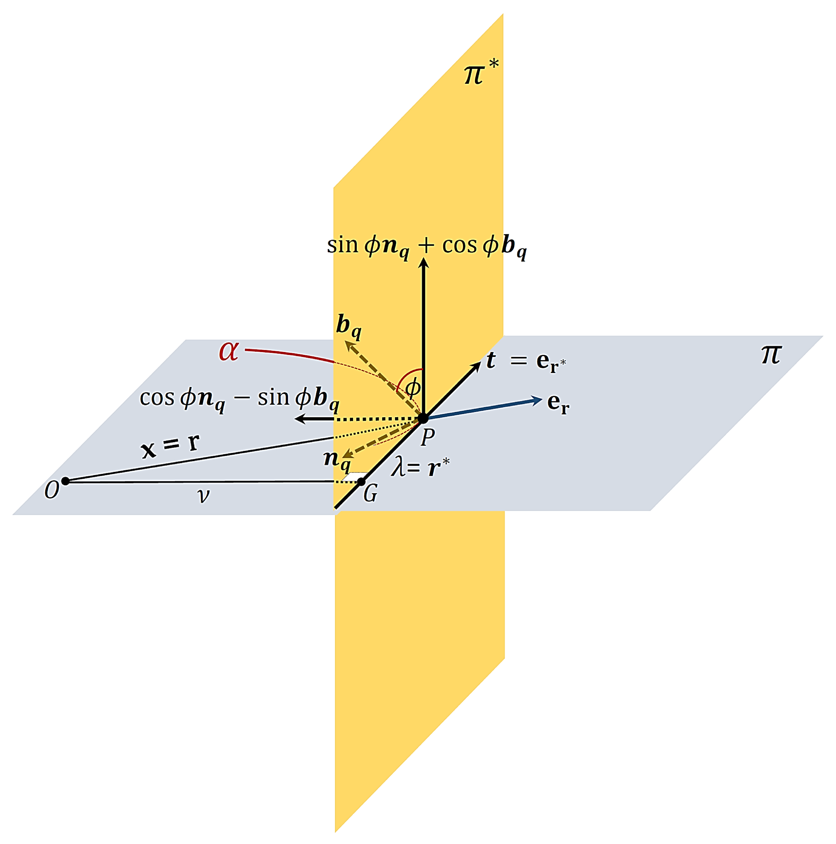
Corollary 1.

In Euclidean 3-space, assume that the oriented quasi curve traced out by the point particle $\mathcal{P}$ is limited to the plane π which does not necessarily contain the origin $\mathcal{O}$. Suppose that the component of the vector ${\mathcal{H}}^{\mathcal{O}}$ along the vector $\left(sin\varphi {\mathbf{N}}_{\mathbf{q}}+cos\varphi {\mathbf{B}}_{\mathbf{q}}\right)$ never vanishes. Then, we can state the following:

-

The tangential and special radial components of the jerk vector become

$$\begin{array}{ccc}\hfill {\mathcal{T}}_{\mathbf{t}}& =& \left(\frac{{\mathrm{d}}^{3}s}{\mathrm{d}{t}^3}\right)-\left({\kappa }_1^2+{\kappa }_2^2\right){\left(\frac{\mathrm{d}s}{\mathrm{d}t}\right)}^3+\frac{3\lambda }{\nu }\sqrt{{\kappa }_1^2+{\kappa }_2^2}\left(\frac{\mathrm{d}s}{\mathrm{d}t}\right)\left(\frac{{\mathrm{d}}^{2}s}{\mathrm{d}{t}^2}\right)\hfill \\ & & +\frac{\lambda }{\nu }{\left(\frac{\mathrm{d}s}{\mathrm{d}t}\right)}^3\frac{\mathrm{d}}{\mathrm{d}s}\left(\sqrt{{\kappa }_1^2+{\kappa }_2^2}\right),\hfill \\ \hfill {\mathcal{T}}_{\mathbf{r}}& =& -\frac{3r}{\nu }\sqrt{{\kappa }_1^2+{\kappa }_2^2}\left(\frac{\mathrm{d}s}{\mathrm{d}t}\right)\left(\frac{{\mathrm{d}}^{2}s}{\mathrm{d}{t}^2}\right)-\frac{r}{\nu }{\left(\frac{\mathrm{d}s}{\mathrm{d}t}\right)}^3\frac{\mathrm{d}}{\mathrm{d}s}\left(\sqrt{{\kappa }_1^2+{\kappa }_2^2}\right),\hfill \\ \hfill {\mathcal{T}}_{{\mathbf{r}}^{*}}& =& 0.\hfill \end{array}$$

(26)

-

The tangential and special radial components of the snap vector become

$$\begin{array}{ccc}\hfill {\mathcal{F}}_{\mathbf{t}}& =& \left(\frac{{\mathrm{d}}^{4}s}{\mathrm{d}{t}^4}\right)-6\left({\kappa }_1^2+{\kappa }_2^2\right){\left(\frac{\mathrm{d}s}{\mathrm{d}t}\right)}^2\left(\frac{{\mathrm{d}}^{2}s}{\mathrm{d}{t}^2}\right)-3\sqrt{{\kappa }_1^2+{\kappa }_2^2}{\left(\frac{\mathrm{d}s}{\mathrm{d}t}\right)}^4\frac{\mathrm{d}}{\mathrm{d}s}\left(\sqrt{{\kappa }_1^2+{\kappa }_2^2}\right)\hfill \\ & & +\frac{4\lambda }{\nu }\sqrt{{\kappa }_1^2+{\kappa }_2^2}\left(\frac{\mathrm{d}s}{\mathrm{d}t}\right)\left(\frac{{\mathrm{d}}^{3}s}{\mathrm{d}{t}^3}\right)+\frac{6\lambda }{\nu }{\left(\frac{\mathrm{d}s}{\mathrm{d}t}\right)}^2\left(\frac{{\mathrm{d}}^{2}s}{\mathrm{d}{t}^2}\right)\frac{\mathrm{d}}{\mathrm{d}s}\left(\sqrt{{\kappa }_1^2+{\kappa }_2^2}\right)\hfill \\ & & +\frac{3\lambda }{\nu }\sqrt{{\kappa }_1^2+{\kappa }_2^2}{\left(\frac{{\mathrm{d}}^{2}s}{\mathrm{d}{t}^2}\right)}^2+\frac{\lambda }{\nu }{\left(\frac{\mathrm{d}s}{\mathrm{d}t}\right)}^4\frac{{\mathrm{d}}^2}{\mathrm{d}{s}^2}\left(\sqrt{{\kappa }_1^2+{\kappa }_2^2}\right)\hfill \\ & & -\frac{\lambda }{\nu }{\left({\kappa }_1^2+{\kappa }_2^2\right)}^{3/2}{\left(\frac{\mathrm{d}s}{\mathrm{d}t}\right)}^4,\hfill \\ \hfill {\mathcal{F}}_{\mathbf{r}}& =& -\frac{4r}{\nu }\sqrt{{\kappa }_1^2+{\kappa }_2^2}\left(\frac{\mathrm{d}s}{\mathrm{d}t}\right)\left(\frac{{\mathrm{d}}^{3}s}{\mathrm{d}{t}^3}\right)-\frac{6r}{\nu }{\left(\frac{\mathrm{d}s}{\mathrm{d}t}\right)}^2\left(\frac{{\mathrm{d}}^{2}s}{\mathrm{d}{t}^2}\right)\frac{\mathrm{d}}{\mathrm{d}s}\left(\sqrt{{\kappa }_1^2+{\kappa }_2^2}\right)\hfill \\ & & -\frac{3r}{\nu }\sqrt{{\kappa }_1^2+{\kappa }_2^2}{\left(\frac{{\mathrm{d}}^{2}s}{\mathrm{d}{t}^2}\right)}^2-\frac{r}{\nu }{\left(\frac{\mathrm{d}s}{\mathrm{d}t}\right)}^4\frac{{\mathrm{d}}^2}{\mathrm{d}{s}^2}\left(\sqrt{{\kappa }_1^2+{\kappa }_2^2}\right)\hfill \\ & & +\frac{r}{\nu }{\left({\kappa }_1^2+{\kappa }_2^2\right)}^{3/2}{\left(\frac{\mathrm{d}s}{\mathrm{d}t}\right)}^4,\hfill \\ \hfill {\mathcal{F}}_{{\mathbf{r}}^{*}}& =& 0.\hfill \end{array}$$

(27)

Proof. 

Let a point particle $\mathcal{P}$ move along an arc-length parameterized quasi curve $\alpha \left(s\right)$ that lies in the plane $\pi$ and choose a fixed origin $\mathcal{O}$ in the space ${\mathbb{E}}^3$. Then, there are two cases. Firstly, we assume that the plane $\pi$ does not contain $\mathcal{O}$. Then, $\mu \ne 0$. Through an assumption “the component of the vector ${\mathcal{H}}^{\mathcal{O}}$ along the vector $\left(sin\varphi {\mathbf{N}}_{\mathbf{q}}+cos\varphi {\mathbf{B}}_{\mathbf{q}}\right)$ in (22) never vanishes”. Then $\nu \ne 0$. We know that $\tau =0$ in the planar motion. Then, the vector $\left(sin\varphi {\mathbf{N}}_{\mathbf{q}}+cos\varphi {\mathbf{B}}_{\mathbf{q}}\right)$ is constant and perpendicular to the plane $\pi$. Therefore, $\mu$ is a nonzero constant and

$${\left(sin\varphi {\mathbf{N}}_{\mathbf{q}}+cos\varphi {\mathbf{B}}_{\mathbf{q}}\right)}^{\prime }=0.$$

By means of (7) and (8), we obtain

$$-\left[\left({\kappa }_3-{\varphi }^{\prime }\right)cos\varphi \right]{\mathbf{N}}_{\mathbf{q}}+\left[\left({\kappa }_3-{\varphi }^{\prime }\right)sin\varphi \right]{\mathbf{B}}_{\mathbf{q}}=0,$$

which implies that

$${\kappa }_3-{\varphi }^{\prime }=0.$$

Consequently, we find from (14) and (15) that the tangential and special radial components of the jerk and snap vectors are expressed as in (26) and (27), respectively. Secondly, we assume that the plane $\pi$ contains $\mathcal{O}$. Then, $\mu =0$. As well, $\nu \ne 0$ and ${\kappa }_3-{\varphi }^{\prime }=0$. Thus, the quantities

$$-\frac{\lambda {\left({\kappa }_3-{\varphi }^{\prime }\right)}^2}{\nu }\sqrt{{\kappa }_1^2+{\kappa }_2^2}{\left(\frac{\mathrm{d}s}{\mathrm{d}t}\right)}^4$$

and

$$\frac{r{\left({\kappa }_3-{\varphi }^{\prime }\right)}^2}{\nu }\sqrt{{\kappa }_1^2+{\kappa }_2^2}{\left(\frac{\mathrm{d}s}{\mathrm{d}t}\right)}^4$$

vanish. While, the quantities

$$\begin{array}{ccc}& & -\frac{6\lambda \left({\kappa }_3-{\varphi }^{\prime }\right)}{\mu }\sqrt{{\kappa }_1^2+{\kappa }_2^2}{\left(\frac{\mathrm{d}s}{\mathrm{d}t}\right)}^2\left(\frac{{\mathrm{d}}^{2}s}{\mathrm{d}{t}^2}\right),\frac{6r^{*}\left({\kappa }_3-{\varphi }^{\prime }\right)}{\mu }\sqrt{{\kappa }_1^2+{\kappa }_2^2}{\left(\frac{\mathrm{d}s}{\mathrm{d}t}\right)}^2\left(\frac{{\mathrm{d}}^{2}s}{\mathrm{d}{t}^2}\right),\hfill \\ & & -\frac{2\lambda \left({\kappa }_3-{\varphi }^{\prime }\right)}{\mu }{\left(\frac{\mathrm{d}s}{\mathrm{d}t}\right)}^4\frac{\mathrm{d}}{\mathrm{d}s}\left(\sqrt{{\kappa }_1^2+{\kappa }_2^2}\right),\frac{2r^{*}\left({\kappa }_3-{\varphi }^{\prime }\right)}{\mu }{\left(\frac{\mathrm{d}s}{\mathrm{d}t}\right)}^4\frac{\mathrm{d}}{\mathrm{d}s}\left(\sqrt{{\kappa }_1^2+{\kappa }_2^2}\right),\hfill \\ & & -\frac{\lambda {\left({\kappa }_3-{\varphi }^{\prime }\right)}^{\prime }}{\mu }\sqrt{{\kappa }_1^2+{\kappa }_2^2}{\left(\frac{\mathrm{d}s}{\mathrm{d}t}\right)}^4,\frac{r^{*}{\left({\kappa }_3-{\varphi }^{\prime }\right)}^{\prime }}{\mu }\sqrt{{\kappa }_1^2+{\kappa }_2^2}{\left(\frac{\mathrm{d}s}{\mathrm{d}t}\right)}^4,\hfill \\ & & -\frac{\lambda \left({\kappa }_3-{\varphi }^{\prime }\right)}{\mu }\sqrt{{\kappa }_1^2+{\kappa }_2^2}{\left(\frac{\mathrm{d}s}{\mathrm{d}t}\right)}^3\mathrm{and}\frac{r^{*}\left({\kappa }_3-{\varphi }^{\prime }\right)}{\mu }\sqrt{{\kappa }_1^2+{\kappa }_2^2}{\left(\frac{\mathrm{d}s}{\mathrm{d}t}\right)}^3\hfill \end{array}$$

have indefiniteness $0/0$. Therefore, we will study this case when $\mu ⟶0$. Then, it follows from (18), (19) and (24) that $r^{*}\approx \lambda$ and $\mathbf{T}\approx {\mathbf{e}}_{{\mathbf{r}}^{*}}$. (See Figure 2).

Consequently, we can say that the vectors

$$\left[-\frac{\lambda \left({\kappa }_3-{\varphi }^{\prime }\right)}{\mu }\sqrt{{\kappa }_1^2+{\kappa }_2^2}{\left(\frac{\mathrm{d}s}{\mathrm{d}t}\right)}^3\right]\mathbf{T}+\left[\frac{r^{*}\left({\kappa }_3-{\varphi }^{\prime }\right)}{\mu }\sqrt{{\kappa }_1^2+{\kappa }_2^2}{\left(\frac{\mathrm{d}s}{\mathrm{d}t}\right)}^3\right]{\mathbf{e}}_{{\mathbf{r}}^{*}}$$

and

$$\begin{array}{ccc}& & \left[-\frac{6\lambda \left({\kappa }_3-{\varphi }^{\prime }\right)}{\mu }\sqrt{{\kappa }_1^2+{\kappa }_2^2}{\left(\frac{\mathrm{d}s}{\mathrm{d}t}\right)}^2\left(\frac{{\mathrm{d}}^{2}s}{\mathrm{d}{t}^2}\right)-\frac{\lambda {\left({\kappa }_3-{\varphi }^{\prime }\right)}^{\prime }}{\mu }\sqrt{{\kappa }_1^2+{\kappa }_2^2}{\left(\frac{\mathrm{d}s}{\mathrm{d}t}\right)}^4\right.\hfill \\ & & \left.-\frac{2\lambda \left({\kappa }_3-{\varphi }^{\prime }\right)}{\mu }{\left(\frac{\mathrm{d}s}{\mathrm{d}t}\right)}^4\frac{\mathrm{d}}{\mathrm{d}s}\left(\sqrt{{\kappa }_1^2+{\kappa }_2^2}\right)\right]\mathbf{T}\hfill \\ & & +\left[\frac{6r^{*}\left({\kappa }_3-{\varphi }^{\prime }\right)}{\mu }\sqrt{{\kappa }_1^2+{\kappa }_2^2}{\left(\frac{\mathrm{d}s}{\mathrm{d}t}\right)}^2\left(\frac{{\mathrm{d}}^{2}s}{\mathrm{d}{t}^2}\right)+\frac{r^{*}{\left({\kappa }_3-{\varphi }^{\prime }\right)}^{\prime }}{\mu }\sqrt{{\kappa }_1^2+{\kappa }_2^2}{\left(\frac{\mathrm{d}s}{\mathrm{d}t}\right)}^4\right.\hfill \\ & & \left.+\frac{2r^{*}\left({\kappa }_3-{\varphi }^{\prime }\right)}{\mu }{\left(\frac{\mathrm{d}s}{\mathrm{d}t}\right)}^4\frac{\mathrm{d}}{\mathrm{d}s}\left(\sqrt{{\kappa }_1^2+{\kappa }_2^2}\right)\right]{\mathbf{e}}_{{\mathbf{r}}^{*}}\hfill \end{array}$$

are about to coincide with the zero vector at $\mu ⟶0$. Thus, we find from (14) and (15) that the tangential and special radial components of the jerk and snap vectors are expressed as in (26) and (27), respectively. The proof is complete. □

Remark 3.

If we put ${\kappa }_2=0$ in the previous theorems and corollaries, we obtain resolutions of the jerk and snap vectors for a Frenet curve in Euclidean 3-space.

4. Applications

In this section, we present examples to illustrate our results.

Example 1.

Let us consider a point particle $\mathcal{P}$ moving along a slant helix (see Figure 3)

$$\alpha \left(t\right)=\left(\frac{1}{6}sint+\frac{2}{3}sin\frac{t}{2},\frac{1}{6}cost+\frac{2}{3}cos\frac{t}{2},\frac{4\sqrt{2}}{3}cos\frac{t}{4}\right)$$

in Euclidean 3-space ${\mathbb{E}}^3$. In this case, the position vector $\mathcal{X}$ of $\mathcal{P}$ is given as

$$\mathcal{X}=\left(\frac{1}{6}sint+\frac{2}{3}sin\frac{t}{2},\frac{1}{6}cost+\frac{2}{3}cos\frac{t}{2},\frac{4\sqrt{2}}{3}cos\frac{t}{4}\right),$$

where t indicates time. The velocity $\mathcal{V}$, acceleration $\mathcal{A}$, jerk (jolt) $\mathcal{J}$ and snap (jounce) $\mathcal{S}$ vectors of $\mathcal{P}$ are

$$\begin{array}{ccc}\hfill \mathcal{V}& =& \left(\frac{1}{6}cost+\frac{1}{3}cos\frac{t}{2},-\frac{1}{6}sint-\frac{1}{3}sin\frac{t}{2},-\frac{\sqrt{2}}{3}sin\frac{t}{4}\right),\hfill \\ \hfill \mathcal{A}& =& \left(-\frac{1}{3}sin\frac{3t}{4}cos\frac{t}{4},-\frac{1}{3}cos\frac{3t}{4}cos\frac{t}{4},-\frac{1}{6\sqrt{2}}cos\frac{t}{4}\right),\hfill \\ \hfill \mathcal{J}& =& \left(-\frac{1}{6}cost-\frac{1}{12}cos\frac{t}{2},\frac{1}{6}sint+\frac{1}{12}sin\frac{t}{2},\frac{1}{24\sqrt{2}}sin\frac{t}{4}\right),\hfill \\ \hfill \mathcal{S}& =& \left(\frac{1}{6}sint+\frac{1}{24}sin\frac{t}{2},\frac{1}{6}cost+\frac{1}{24}cos\frac{t}{2},\frac{1}{96\sqrt{2}}cos\frac{t}{4}\right).\hfill \end{array}$$

The speed of $\mathcal{P}$ is

$$∥\mathcal{V}∥=\frac{\mathrm{d}s}{\mathrm{d}t}=\frac{1}{2}.$$

Thus, we have

$$s=s\left(t\right)=\frac{t}{2}$$

and

$$\frac{{\mathrm{d}}^{2}s}{\mathrm{d}{t}^2}=\frac{{\mathrm{d}}^{3}s}{\mathrm{d}{t}^3}=\frac{{\mathrm{d}}^{4}s}{\mathrm{d}{t}^4}=0.$$

It is easy to see that the curve can be reparameterized by the arc-length function as

$${\alpha }^{*}\left(s\right)=\left(\frac{1}{6}sin2s+\frac{2}{3}sins,\frac{1}{6}cos2s+\frac{2}{3}coss,\frac{4\sqrt{2}}{3}cos\frac{s}{2}\right).$$

(28)

From (1), the Frenet frame for the slant helix is

$$\begin{array}{ccc}\hfill \mathbf{T}\left(s\right)& =& \left(\frac{1}{3}cos2s+\frac{2}{3}coss,-\frac{1}{3}sin2s-\frac{2}{3}sins,-\frac{2\sqrt{2}}{3}sin\frac{s}{2}\right),\hfill \\ \hfill \mathbf{N}\left(s\right)& =& \left(-\frac{4}{3\sqrt{2}}sin\frac{3s}{2},-\frac{4}{3\sqrt{2}}cos\frac{3s}{2},-\frac{1}{3}\right),\hfill \\ \hfill \mathbf{B}\left(s\right)& =& \left(-\frac{1}{3}sin2s+\frac{2}{3}sins,-\frac{1}{3}cos2s+\frac{2}{3}coss,-\frac{4}{3\sqrt{2}}cos\frac{s}{2}\right).\hfill \end{array}$$

Thus, the Frenet-curvatures are

$$\kappa \left(s\right)=\sqrt{2}cos\frac{s}{2},\tau \left(s\right)=\sqrt{2}sin\frac{s}{2}.$$

From (8), the quasi-curvatures are

$${\kappa }_1=\sqrt{2}cos\frac{s}{2}cos\varphi ,{\kappa }_2=-\sqrt{2}cos\frac{s}{2}sin\varphi ,{\kappa }_3={\varphi }^{\prime }+\sqrt{2}sin\frac{s}{2}.$$

By using (5), the quasi vectors for the slant helix are given as

$$\begin{array}{ccc}\hfill \mathbf{T}\left(s\right)& =& \left(\frac{1}{3}cos2s+\frac{2}{3}coss,-\frac{1}{3}sin2s-\frac{2}{3}sins,-\frac{2\sqrt{2}}{3}sin\frac{s}{2}\right),\hfill \\ \hfill {\mathbf{N}}_{\mathbf{q}}\left(s\right)& =& \left(-\frac{4}{3\sqrt{2}}sin\frac{3s}{2}cos\varphi -\frac{1}{3}sin2ssin\varphi +\frac{2}{3}sinssin\varphi ,\right.\hfill \\ & & -\frac{4}{3\sqrt{2}}cos\frac{3s}{2}cos\varphi -\frac{1}{3}cos2ssin\varphi +\frac{2}{3}cosssin\varphi ,\hfill \\ & & \left.-\frac{1}{3}cos\varphi -\frac{4}{3\sqrt{2}}cos\frac{s}{2}sin\varphi \right),\hfill \\ \hfill {\mathbf{B}}_{\mathbf{q}}\left(s\right)& =& \left(\frac{4}{3\sqrt{2}}sin\frac{3s}{2}sin\varphi -\frac{1}{3}sin2scos\varphi +\frac{2}{3}sinscos\varphi ,\right.\hfill \\ & & \frac{4}{3\sqrt{2}}cos\frac{3s}{2}sin\varphi -\frac{1}{3}cos2scos\varphi +\frac{2}{3}cosscos\varphi ,\hfill \\ & & \left.\frac{1}{3}sin\varphi -\frac{4}{3\sqrt{2}}cos\frac{s}{2}cos\varphi \right).\hfill \end{array}$$

By means of (17), (19) and (28), we obtain

$$\begin{array}{ccc}\hfill \lambda & =& -sins,\nu =\sqrt{2}cos\frac{s}{2},\mu =-\frac{1+2coss}{2},\hfill \\ \hfill r& =& \sqrt{2\left(2-coss\right)}cos\frac{s}{2},r^{*}=\frac{\sqrt{5+4coss}}{2}.\hfill \end{array}$$

By applying Theorem 1, we obtain the jerk and snap vectors of the point particle $\mathcal{P}$ along the quasi bases as

$$\begin{array}{ccc}\hfill \mathcal{J}& =& \left[-\frac{1}{4}{cos}^2\frac{s}{2}\right]\mathbf{T}+\left[-\frac{1}{8\sqrt{2}}sin\frac{s}{2}cos\varphi +\frac{1}{8}sinssin\varphi \right]{\mathbf{N}}_{\mathbf{q}}\hfill \\ & & +\left[\frac{1}{8\sqrt{2}}sin\frac{s}{2}sin\varphi +\frac{1}{8}sinscos\varphi \right]{\mathbf{B}}_{\mathbf{q}}\hfill \end{array}$$

and

$$\begin{array}{ccc}\hfill \mathcal{S}& =& \left[\frac{3}{32}sins\right]\mathbf{T}+\left[-\frac{9}{32\sqrt{2}}cos\frac{s}{2}cos\varphi -\frac{1}{32}sin\varphi +\frac{3}{32}cosssin\varphi \right]{\mathbf{N}}_{\mathbf{q}}\hfill \\ & & +\left[\frac{9}{32\sqrt{2}}cos\frac{s}{2}sin\varphi -\frac{1}{32}cos\varphi +\frac{3}{32}cosscos\varphi \right]{\mathbf{B}}_{\mathbf{q}},\hfill \end{array}$$

respectively. By applying Theorem 2, we obtain the jerk and snap vectors of the point particle $\mathcal{P}$ along the vectors $\mathbf{T}$, ${\mathbf{e}}_{\mathbf{r}}$ and ${\mathbf{e}}_{{\mathbf{r}}^{*}}$ as

$$\begin{array}{ccc}\hfill \mathcal{J}& =& \left[-\frac{2{cos}^{2}s+5coss+5}{16\left(1+2coss\right)}\right]\mathbf{T}+\left[\frac{\sqrt{2-coss}}{8\sqrt{2}}sin\frac{s}{2}\right]{\mathbf{e}}_{\mathbf{r}}\hfill \\ & & -\left[\frac{\sqrt{5+4coss}}{8\left(1+2coss\right)}sins\right]{\mathbf{e}}_{{\mathbf{r}}^{*}}\hfill \end{array}$$

and

$$\begin{array}{ccc}\hfill \mathcal{S}& =& \left[\frac{19+18coss}{64\left(1+2coss\right)}sins\right]\mathbf{T}+\left[\frac{9\sqrt{2-coss}}{32\sqrt{2}}cos\frac{s}{2}\right]{\mathbf{e}}_{\mathbf{r}}\hfill \\ & & +\left[\frac{\left(1-3coss\right)\sqrt{5+4coss}}{32\left(1+2coss\right)}\right]{\mathbf{e}}_{{\mathbf{r}}^{*}},\hfill \end{array}$$

respectively.

Example 2.

Let us consider a point particle $\mathcal{P}$ moving along the log-spiral curve (see Figure 4)

$$\beta \left(t\right)=\left(e^{\vartheta t}sin\left(\vartheta t\right),e^{\vartheta t}cos\left(\vartheta t\right),0\right)$$

in Euclidean 3-space ${\mathbb{E}}^3$. In this case, the position vector $\mathcal{X}$ of $\mathcal{P}$ is given as

$$\mathcal{X}=\left(e^{\vartheta t}sin\left(\vartheta t\right),e^{\vartheta t}cos\left(\vartheta t\right),0\right),$$

where t indicates time and $\vartheta >0$ is a constant. The velocity $\mathcal{V}$, acceleration $\mathcal{A}$, jerk (jolt) $\mathcal{J}$ and snap (jounce) $\mathcal{S}$ vectors of $\mathcal{P}$ are

$$\begin{array}{ccc}\hfill \mathcal{V}& =& \vartheta \left(e^{\vartheta t}sin\left(\vartheta t\right)+e^{\vartheta t}sin\left(\vartheta t\right),e^{\vartheta t}cos\left(\vartheta t\right)-e^{\vartheta t}sin\left(\vartheta t\right),0\right),\hfill \\ \hfill \mathcal{A}& =& 2{\vartheta }^2\left(e^{\vartheta t}cos\left(\vartheta t\right),-e^{\vartheta t}sin\left(\vartheta t\right),0\right),\hfill \\ \hfill \mathcal{J}& =& 2{\vartheta }^3\left(e^{\vartheta t}cos\left(\vartheta t\right)-e^{\vartheta t}sin\left(\vartheta t\right),-e^{\vartheta t}sin\left(\vartheta t\right)-e^{\vartheta t}cos\left(\vartheta t\right),0\right),\hfill \\ \hfill \mathcal{S}& =& -4{\vartheta }^4\left(e^{\vartheta t}sin\left(\vartheta t\right),e^{\vartheta t}cos\left(\vartheta t\right),0\right).\hfill \end{array}$$

The speed of $\mathcal{P}$ is

$$∥\mathcal{V}∥=\frac{\mathrm{d}s}{\mathrm{d}t}=\sqrt{2}\vartheta e^{\vartheta t}.$$

Thus, we have

$$s=s\left(t\right)=\sqrt{2}{e}^{\vartheta t}-\sqrt{2}$$

and

$$\frac{{\mathrm{d}}^{2}s}{\mathrm{d}{t}^2}=\sqrt{2}{\vartheta }^2{e}^{\vartheta t},\frac{{\mathrm{d}}^{3}s}{\mathrm{d}{t}^3}=\sqrt{2}{\vartheta }^3{e}^{\vartheta t},\frac{{\mathrm{d}}^{4}s}{\mathrm{d}{t}^4}=\sqrt{2}{\vartheta }^4{e}^{\vartheta t}.$$

It is easy to see that the curve can be reparameterized by the arc-length function as

$${\beta }^{*}\left(s\right)=\left(s/\sqrt{2}+1\right)\left(sinlog\left(s/\sqrt{2}+1\right),coslog\left(s/\sqrt{2}+1\right),0\right).$$

(29)

From (1), the Frenet frame for the log-spiral curve is

$$\begin{array}{ccc}\hfill \mathbf{T}\left(s\right)& =& \frac{1}{\sqrt{2}}\left(sinlog\left(s/\sqrt{2}+1\right)+coslog\left(s/\sqrt{2}+1\right)\right.\hfill \\ & & \left.,coslog\left(s/\sqrt{2}+1\right)-sinlog\left(s/\sqrt{2}+1\right),0\right),\hfill \\ \hfill \mathbf{N}\left(s\right)& =& \frac{1}{\sqrt{2}}\left(coslog\left(s/\sqrt{2}+1\right)-sinlog\left(s/\sqrt{2}+1\right)\right.\hfill \\ & & \left.,-sinlog\left(s/\sqrt{2}+1\right)-coslog\left(s/\sqrt{2}+1\right),0\right),\hfill \\ \hfill \mathbf{B}\left(s\right)& =& \left(0,0,-1\right).\hfill \end{array}$$

Thus, the Frenet-curvatures are

$$\kappa \left(s\right)=\frac{1}{s+\sqrt{2}},\tau \left(s\right)=0.$$

From (8), the quasi-curvatures are

$${\kappa }_1=\frac{1}{s+\sqrt{2}}cos\varphi ,{\kappa }_2=-\frac{1}{s+\sqrt{2}}sin\varphi ,{\kappa }_3={\varphi }^{\prime }.$$

By using (5), the quasi vectors for the log-spiral curve are given as

$$\begin{array}{ccc}\hfill \mathbf{T}\left(s\right)& =& \frac{1}{\sqrt{2}}\left(sinlog\left(s/\sqrt{2}+1\right)+coslog\left(s/\sqrt{2}+1\right)\right.\hfill \\ & & \left.,coslog\left(s/\sqrt{2}+1\right)-sinlog\left(s/\sqrt{2}+1\right),0\right),\hfill \\ \hfill {\mathbf{N}}_{\mathbf{q}}\left(s\right)& =& \frac{1}{\sqrt{2}}\left(coslog\left(s/\sqrt{2}+1\right)cos\varphi -sinlog\left(s/\sqrt{2}+1\right)cos\varphi \right.\hfill \\ & & \left.,-sinlog\left(s/\sqrt{2}+1\right)cos\varphi -coslog\left(s/\sqrt{2}+1\right)cos\varphi ,-\sqrt{2}sin\varphi \right),\hfill \\ \hfill {\mathbf{B}}_{\mathbf{q}}\left(s\right)& =& \frac{1}{\sqrt{2}}\left(-coslog\left(s/\sqrt{2}+1\right)sin\varphi +sinlog\left(s/\sqrt{2}+1\right)sin\varphi \right.\hfill \\ & & \left.,sinlog\left(s/\sqrt{2}+1\right)sin\varphi +coslog\left(s/\sqrt{2}+1\right)sin\varphi ,-\sqrt{2}cos\varphi \right).\hfill \end{array}$$

By means of (17), (19) and (29), we obtain

$$\lambda =\nu =r^{*}=\frac{s+\sqrt{2}}{2},\mu =0,r=\frac{s+\sqrt{2}}{\sqrt{2}}.$$

respectively. By applying Corollary 1, we obtain the tangential and special radial components of the jerk and snap vectors as

$${\mathcal{T}}_{\mathbf{t}}=2\sqrt{2}{\vartheta }^3{e}^{\vartheta t},{\mathcal{T}}_{\mathbf{r}}=-4{\vartheta }^3{e}^{\vartheta t},{\mathcal{T}}_{{\mathbf{r}}^{*}}=0$$

and

$${\mathcal{F}}_{\mathbf{t}}=0,{\mathcal{F}}_{\mathbf{r}}=-4{\vartheta }^4{e}^{\vartheta t},{\mathcal{F}}_{{\mathbf{r}}^{*}}=0,$$

respectively.

5. Conclusions

In this article, by employing the quasi frame, resolutions of the jerk and snap vectors of a point particle moving along a curve in Euclidean 3-space were studied. In detail, the jerk and snap vectors of the point particle along the tangential, quasi-normal and quasi-binormal directions were obtained. An alternative approach of the jerk and snap vectors along the tangential direction and two special radial directions was presented. Moreover, the components of the jerk and snap vectors for the planar motion in Euclidean 3-space were discussed as corollary.

References

1. Eager, D.; Pendrill, A.M.; Reistad, N. Beyond velocity and acceleration: Jerk, snap and higher derivatives. Eur. J. Phys. 2016, 37, 065008. [Google Scholar] [CrossRef]
2. Siczek, K.; Stefański, A. Analysis of dynamics and friction resistance in the cam-tappet system. J. Theor. Appl. Mech. 2019, 57, 273–286. [Google Scholar] [CrossRef]
3. Sajjadi, S.S.; Baleanu, D.; Jajarmi, A.; Pirouz, H.M. A new adaptive synchronization and hyperchaos control of a biological snap oscillator. Chaos Solitons Fractals 2020, 138, 109919. [Google Scholar] [CrossRef]
4. Siacci, F. Moto per Una Linea Gobba; Atti R Accad Sci: Torino, Italy, 1879. [Google Scholar]
5. Whittaker, E.T. A Treatise on the Analytical Dynamics of Particles and Rigid Bodies; Cambridge University Press: New York, NY, USA, 1944. [Google Scholar]
6. Grossman, N. The Sheer Joy of Celestial Mechanics; Springer Science & Business Media: Berlin/Heidelberg, Germany, 1996. [Google Scholar]
7. Casey, J. Siacci’s resolution of the acceleration vector for a space curve. Meccanica 2011, 46, 471–476. [Google Scholar] [CrossRef] [Green Version]
8. Küçükarslan, Z.; Yılmaz, M.Y.; Bektas, M. Siacci’s theorem for curves in Finsler manifold F3. Turk. J. Sci. Technol. 2012, 7, 181–185. [Google Scholar]
9. Özen, K.E.; Tosun, M.; Akyigit, M. Siacci’s theorem according to Darboux frame. An. St. Univ. Ovidius Constanta 2017, 25, 155–165. [Google Scholar]
10. Özen, K.E. Siacci’s theorem for Frenet curves in Minkowski 3-space. Math. Sci. Appl. E-Notes 2020, 8, 159–167. [Google Scholar] [CrossRef]
11. Résal, H. Traité de Cinématique Pure; Mallet-Bachelier: Paris, France, 1862. [Google Scholar]
12. Özen, K.E.; Dündar, F.S.; Tosun, M. An alternative approach to jerk in motion along a space curve with applications. J. Theor. Appl. Mech. 2019, 57, 435–444. [Google Scholar] [CrossRef]
13. Özen, K.E.; Güner, M.; Tosun, M. A note on the acceleration and jerk in motion along a space curve. An. St. Univ. Ovidius Constanta 2020, 28, 151–164. [Google Scholar] [CrossRef]
14. Güner, M. On the jerk in motion along a space curve. Math. Methods Appl. Sci. 2021, 44, 7407–7415. [Google Scholar] [CrossRef]
15. Tosun, M.; Hızarcıoglu, M. On the jerk in motion along a regular surface curve. TBILISI-MATHEMATICS 2020, 3, 67–75. [Google Scholar]
16. Tsirlin, M. Jerk by axes in motion along a space curve. J. Theor. Appl. Mech. 2017, 55, 1437–1441. [Google Scholar] [CrossRef] [Green Version]
17. Elsharkawy, A.; Elshenhab, A. On the acceleration and jerk in motion along a space curve with quasi-frame in Euclidean 3-space. Authorea 2020. [Google Scholar] [CrossRef]
18. Do Carmo, M.P. Differential Geometry of Curves and Surfaces; Prentice Hall: Englewood Cliffs, NJ, USA, 1976. [Google Scholar]
19. Dede, M.; Ekici, C.; Görgülü, A. Directional q-frame along a space curve. IJARC SSE 2015, 5, 775–780. [Google Scholar]
20. Dede, M.; Ekici, C.; Tozak, H. Directional tubular surfaces. Int. J. Algebra 2015, 9, 527–535. [Google Scholar] [CrossRef] [Green Version]
Figure 1. The motion of point particle P along a quasi curve α in E 3 .
Mathematics 09 03128 g001
Figure 2. The motion of point particle P along a quasi plane curve α that contains a fixed origin O .
Mathematics 09 03128 g002
Figure 3. The slant helix curve.
Mathematics 09 03128 g003
Figure 4. The log-spiral curve.
Mathematics 09 03128 g004
Publisher’s Note: MDPI stays neutral with regard to jurisdictional claims in published maps and institutional affiliations.