Runge–Kutta Pairs of Orders 5(4) Trained to Best Address Keplerian Type Orbits

Abstract

The derivation of Runge–Kutta pairs of orders five and four that effectively uses six stages per step is considered. The coefficients provided by such a method are 27 and have to satisfy a system of 25 nonlinear equations. Traditionally, various solutions have been tried. Each of these solutions makes use of some simplified assumptions and offers different families of methods. Here, we make use of the most celebrated family to appear in the literature, where we may use as the last stage the first function evaluation from the next step (FSAL property). The family under consideration has the advantage of being solved explicitly. Actually, we arrive at a subsystem where all the coefficients are found with respect to five free parameters. These free parameters are adjusted (trained) in order to deliver a pair that outperforms other similar pairs of orders $5(4)$ in Keplerian type orbits, e.g., Kepler, perturbed Kepler, Arenstorf orbit or Pleiades. The training uses differential evolution technique. The finally proposed pair has a remarkable performance and offers on average more than a digit of accuracy in a variety of orbits.

1. Introduction

A system of ordinary differential equations of the form

$$x^{\prime }=f(t,x),x(t_0)=x_0$$

(1)

with $t_0\in \mathbb{R}$, $x,x^{\prime }\in {\mathbb{R}}^m$ and $f:\mathbb{R}\times {\mathbb{R}}^m\to {\mathbb{R}}^m$, is called Initial Value problem (IVP).

For addressing the above problem (1), we usually try Runge–Kutta (RK) pairs, which is perhaps the most popular choice among the numerical methods. These pairs are compactly presented by the Butcher tableau [1,2] that follows,

$$\begin{array}{cc}\hfill q& D\\ \hfill & w\\ \hfill & \widehat{w}\end{array}$$

with $w^T,{\widehat{w}}^T,q\in R^s$ and $D\in R^{s\times s}.$ This method spends s function evaluations per step that are evaluated explicitly when D is a strictly lower triangular. The estimate of the solution steps from $(t_k,x_k)$ to $t_{k+1}=t_k+h_k$ after producing two approximations for $x(t_{k+1}).$ Namely, $x_{k+1}$ and ${\widehat{x}}_{k+1}$, given by

$$x_{k+1}=x_k+h_k\sum _{i=1}^s{w}_i{f}_i$$

and

$${\widehat{x}}_{k+1}=x_k+h_k\sum _{i=1}^s{\widehat{w}}_i{f}_i$$

with

$$f_i=f(t_k+q_i{h}_k,x_k+h_k\sum _{j=1}^{i-1}{d}_{ij}{f}_j),$$

for $i=1,\cdots ,s.$ These two estimations $x_{k+1}$ and ${\widehat{x}}_{k+1}$ are, respectively, of algebraic orders $p_1$ and $p_2<p_1$. Thus, in every step, we form the quantity

$${ϵ}_k=h_k^{p_1-p_2-1}·\parallel x_{k+1}-{\widehat{x}}_{k+1}\parallel ,$$

and it is supposed to be an estimate of the local error. Actually, it is used in a step-size changing algorithm

$$h_{k+1}=0.9·h_k^{}·{(\frac{\kappa }{{ϵ}_k})}^{1/p_1},$$

where $\kappa$ is a small enough positive tolerance set by the user. Whenever ${ϵ}_k<\kappa$ we use the above formula for setting the length of the next step forward, i.e., from $t_{k+1}$ to $t_{k+2}$. On the contrary, the same formula is used, but then $h_{k+1}$ is changed with $h_k$ since we have to estimate a new smaller step size for advancing from the current point $t_k$ to a new point $t_k+h_k$. Details in this subject are given in [3]. An abbreviation for these methods is the terminology $RK{p}_1(p_2)$ pairs.

Runge was the first to present a second order RK method by combining a sequence of Euler formulas [4]. Some years later, Kutta managed to construct a four stages fourth order method [5]. Since the system of order conditions required to be solved (see [6]) is too complicated, there was a rather slow progress in the issue. Nyström showed the correct coefficients of a six stages method of fifth order [7]. Higher order methods appeared in the 50s. Huta gave a sixth order method at a cost of eight stages per step [8]. RK pairs were introduced in the 60s. It was E. Fehlberg who constructed at first a series of celebrated pairs of orders 5(4), 6(5) and 8(7), [9,10]. His pioneering work followed in the early 80s by Dormand and Prince who presented their famous pairs [11,12]. Our research group has also derived a series of interesting RK pairs [13,14,15,16].

Almost every non-stiff problem of the form (1) may be solved effectively with RK pairs. The accuracy required explains the wide range of pairs. As a result, the lowest RK pairs are more efficient the lower the accuracy on demand. A high order pair, on the other hand, should be chosen for demanding accuracies at quadruple precision [17].

We’ll concentrate on RK5(4) pairs, which are best for intermediate accuracies. Problems (1) with structure similar to Keplerian forms are of particular interest to us. As a result, we shall offer a specific RK5(4) pair for dealing with this type of cases.

2. Families of Runge–Kutta Pairs of Orders 5(4)

Runge–Kutta pairs of algebraic orders five and four are perhaps the most famed. Their coefficients have to satisfy 25 order conditions. As a result, over time, families of solutions have been developed. The minimum number of stages required to construct a fifth-order RK method or a 5(4) pair is known to be six [1].

Usually these pairs are constructed according to various types of simplifications. After these simplified assumptions applied to the original equations (order conditions), we arrive at a simpler system where some coefficients remain as free parameters. The values of these free parameters were chosen by Fehlberg for minimization the truncation error coefficients of the pair’s fourth-order formula. After considerable numerical testing, Shampine in [18] concluded that propagating the higher-order solution (i.e., here, the fifth order) of a pair is desirable from a numerical standpoint. This technique is called Local Extrapolation.

Dormand and Prince went on to expand a family of fifth-order methods already presented by Butcher in [1]. They suggested a family that borrows the first function evaluation from the next step to embed a fourth-order method within a fifth-order method at no additional cost [11]. For a long time, the best fifth-order pair was commonly considered to be DP5(4), an individual pair in their four-parameter family with small truncation error coefficients of its fifth-order formula. Later on, Papakostas and Papageorgiou extended this family by adding a parameter more [19]. The later authors presented a pair with minimal truncation coefficients and claimed that its performance was in average about $15.8\%$ more efficient than DP5(4) in the standard IVP test set named DETEST [20].

Ten years ago, Tsitouras presented a new family that makes use of the least simplifying assumptions possible [15]. Only the assumptions

$$D·e=q,\mathrm{and}w·\left(D+Q-I_s\right)=\mathbf{0}\in {\mathbb{R}}^{1\times s},$$

with $e=[1,1,\cdots ,1]\in {\mathbb{R}}^s$, $Q=diag(q),I_s\in {\mathbb{R}}^{s\times s}$ the identity matrix, were made there.

The common set of simplifications

$$D·q=\frac{q^2}{2}\mathrm{and}{w}_2=0,$$

is not used. In the above, we set as

$$q^{\tau }=\underset{\tau \mathrm{times}}{\underbrace{q\ast q\ast \cdots \ast q}},$$

the component-wise multiplication among the elements of q. Generally, in the following, by $v\ast u$ we mean the component by component multiplication among matrices with the same number of rows.

Here, we will make use of the five parameters family introduced in [19]. The choice is justified, since this family of solutions is a superset of the solutions given by [11]. Besides, the derivation of the coefficients is explicit and therefore cheap. Meanwhile, the family given in [15], although groundbreaking, is implicit. Thus, the later technique of solutions is somewhat expensive for our goals here.

In the following, we describe the derivation of the coefficients according to the guidelines given in [19].

Notice that, at first, $q_1=0,q_6=q_7=1,w_2={\widehat{w}}_2=w_7=0$ and $d_{ij}=0$ for $i\ge j$.

Set arbitrary values for $q_2\ne 0,q_3,c_4,q_5,{\widehat{w}}_7\ne 0.$$q_3,q_4,q_5$ has to be different from each other and not equal to 1.

• Solve $w·e=1,w·q=\frac{1}{2},w·q^2=\frac{1}{3},w·q^3=\frac{1}{4},w·q^4=\frac{1}{5},$ for $w_1,w_3,w_4,w_5,w_6.$
• Set ${\widehat{w}}_6=\frac{\left(\begin{array}{c}35q_3^2{q}_4-26q_3{q}_4\\ -3q_3+6q_4\end{array}\right)·\left(\begin{array}{c}30q_3{q}_4{q}_5-20q_3{q}_4-20q_3{q}_5+15q_3\\ -20q_4{q}_5+15q_4+15q_5-12\end{array}\right)}{\left\{\begin{array}{c}300(q_3-1)(q_4-1)(q_5-1)·\\ \left(10q_3^2{q}_4-8q_3{q}_4-q_3+2q_4\right)\end{array}\right\}}.$
• Solve $\widehat{w}·e=1,\widehat{w}·q=\frac{1}{2},\widehat{w}·q^2=\frac{1}{3},\widehat{w}·q^3=\frac{1}{4},$ for ${\widehat{w}}_1,{\widehat{w}}_3,{\widehat{w}}_4,{\widehat{w}}_5.$
• Solve $\left\{\begin{array}{ccc}{\left(D·q\right)}_3=0,& {\left(D·q\right)}_4=0,& {\left(D·q\right)}_5=0,\\ {\left(D·q\right)}_6=0,& w·{\left(D+Q-I\right)}_5=0,& {\left(w·D\right)}_2=0,\\ w·{\left(q\ast D\right)}_2=0,& {\left(\widehat{w}·D\right)}_2=0,& w·D·q^3=\frac{1}{20},\\ w·\left(q\ast D\right)·q^2=\frac{1}{15},& \end{array}\right\}$ for $d_{32},d_{42},d_{43},d_{52},d_{53},d_{54},d_{62},d_{63},d_{64}$ and $d_{65}.$ By ${(·)}_j$ is meant the $j-$th component of the underlying vector.

Then set $d_{21}=q_2,d_{31}=q_3-d_{32},d_{41}=q_4-d_{42}-d_{43},$ $d_{51}=q_5-d_{52}-d_{53}-d_{54}$ and $d_{61}=q_6-d_{62}-d_{63}-d_{64}-d_{65}.$

Finally, the FSAL (First Stage As Last) property holds, and

$$d_{7j}=w_j,j=1,2,\cdots ,6.$$

Because the seventh stage is used as the initial stage of the following step, even if $s=7$, the family only spends six stages every step.

The challenge now is how to choose the free parameters. The norm of the principal coefficients of the local truncation error is traditionally minimized. i.e., the terms of $h^6$ in the residual of Taylor error expansions corresponding to the fifth order method of the underlying RK pair [13].

Since our concern here is to deal with Keplerian type orbits, we shall try another approach and train these free parameters in order for the resulting pair to perform best in our problems of interest.

3. Comparison of the Results among Pairs

Comparison of the results observed by various pairs is an interesting issue. It is of crucial importance in our present work. So, let us work on Kepler problem. This has the following form:

$$\begin{array}{c}{}^1{x}^{\prime }={}^{3}x,\hfill \\ {}^2{x}^{\prime }={}^{4}x,\hfill \\ {}^3{x}^{\prime }=-{\displaystyle \frac{{}^{1}x}{{\left(\sqrt{{{(}^{1}x)}^2+{{(}^{2}x)}^2}\right)}^3}},\hfill \\ {}^4{x}^{\prime }=-{\displaystyle \frac{{}^{2}x}{{\left(\sqrt{{{(}^{1}x)}^2+{{(}^{2}x)}^2}\right)}^3}},\hfill \end{array}$$

with $t\in [0,10\pi ]$, $x(0)={\left[1-\gamma ,0,0,\sqrt{\frac{1+\gamma }{1-\gamma }}\right]}^T$ and the theoretical solution

$${}^{1}x(t)=cos(v)-\gamma ,{}^{2}x(t)=sin(v)\sqrt{1-{\gamma }^2}.$$

In the above, $v=\gamma ·sin(u)+x$, $\gamma$ is the eccentricity, and the the left superscript denotes the components of x. They shall not be confused with $x_1={\left[{}^1{x}_1{,}^2{x}_1{,}^3{x}_1{,}^4{x}_1\right]}^T,$$x_2={\left[{}^1{x}_2{,}^2{x}_2{,}^3{x}_2{,}^4{x}_2\right]}^T,x_3,\cdots$, that correspond to the vectors approximating the solution at $t_1,t_2,t_3,\cdots$.

When running DP5(4) for $\gamma =0.6$ and tolerances ${10}^{-5}$, ${10}^{-6},\cdots$, ${10}^{-11}$, we get the results summarized in

Table 1. Results of DP5(4) over Kepler orbit for $\gamma =0.6$.

Tolerance	Stages	End-Point Error
${10}^{-5}$	1033	$2.0\times {10}^{-2}$
${10}^{-6}$	1471	$9.7\times {10}^{-5}$
${10}^{-7}$	2107	$7.85\times {10}^{-5}$
${10}^{-8}$	2689	$8.4\times {10}^{-6}$
${10}^{-9}$	4261	$1.3\times {10}^{-6}$
${10}^{-10}$	6775	$1.4\times {10}^{-7}$
${10}^{-11}$	10,681	$1.4\times {10}^{-8}$

. There we recorded the error observed at the end-point as long as the function evaluations are taken by the pair.

Then, we try T5(4) pair given in [15] and get the results presented in

Table 2. Results of T5(4) over Kepler orbit for $\gamma =0.6$.

Tolerance	Stages	End-Point Error
${10}^{-5}$	1225	$5.0\times {10}^{-3}$
${10}^{-6}$	1795	$6.3\times {10}^{-4}$
${10}^{-7}$	2365	$7.0\times {10}^{-5}$
${10}^{-8}$	3181	$8.8\times {10}^{-6}$
${10}^{-9}$	4963	$9.4\times {10}^{-7}$
${10}^{-10}$	7861	$9.5\times {10}^{-8}$
${10}^{-11}$	12,451	$9.5\times {10}^{-9}$

.

Which pair is more efficient? How can we derive this? Of course, we may not simply check the errors after each tolerance since the number of stages differ. We want to eliminate the presence of tolerances. They do not offer something in comparing the results. We proceed in a way similar to that proposed in [20].

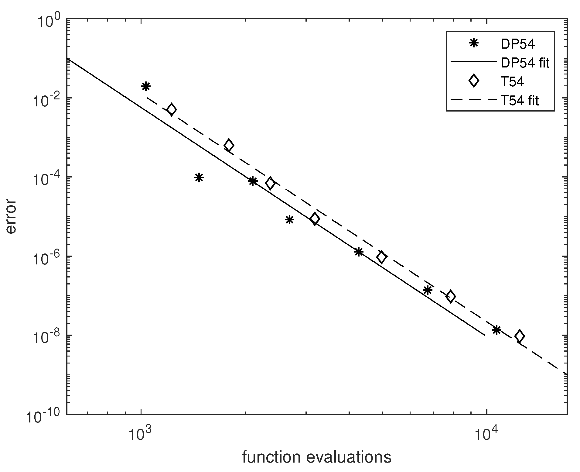
Thus, we form a linear least squares fit on the logarithms of data (i.e., stages and errors). Then, we arrive at a slope that justifies the order of the method. These parallel slopes for DP5(4) and PP5(4) can be seen in Figure 1. See ([2], p. 214) for details in the issue.

Now, we are able to compare the results of the pairs in the selected problem.

In

Table 3. Stages that might have been spent for achieving various errors by both pairs for Keplerian orbit with eccentricity $\gamma =0.6$. Stars indicate unavailability of data to attain the perspective errors.

Expected End-Point Error	DP$5(4)$	T$5(4)$	Efficiency Ratio
${10}^{-1}$	$609.34$	*	*
${10}^{-2}$	$907.08$	$1041.53$	$0.87$
${10}^{-3}$	$1350.31$	$1553.40$	$0.87$
${10}^{-4}$	$2010.11$	$2316.84$	$0.87$
${10}^{-5}$	$2992.11$	$3455.47$	$0.87$
${10}^{-6}$	$4454.45$	$5133.70$	$0.86$
${10}^{-7}$	$6631.02$	$7686.53$	$0.86$
${10}^{-8}$	$9871.14$	$11,$$464.14$	$0.86$
${10}^{-9}$	*	$17,$$098.30$	*

, we present the functions evaluations that might have been spend for achieving various errors by both pairs. These numbers come after the linear fit as explained in [20], while the constant ratio is explained by the parallel slopes among methods of the same order. The later observation might not be present for every problem. Some special characteristics of various problems may exploited differently by various pairs of the same orders and thus may give steeper slopes than expected. Thus, the numbers in the second column of Table 3 are evaluated as

$$\mathrm{stages}\approx {10}^{-0.1728·{log}_{10}(\mathrm{expected}\mathrm{error})+2.6121},$$

while the stages in the third column can be found by the relation

$$\mathrm{stages}\approx {10}^{-0.1736·{log}_{10}(\mathrm{expected}\mathrm{error})+2.6705}.$$

In conclusion, DP5(4) is considered to be 13–14% cheaper than T5(4) in the problem under consideration. After this, we may ask for free parameters that may produce a new pair that is cheaper in a wider class of Keplerian type orbits.

Both methods outperformed their order expectations for this problem. According to theoretical aspects, a fifth order method is expected to perform as

$$\mathrm{stages}={10}^{-\frac{1}{5}·{log}_{10}(\mathrm{expected}\mathrm{error})+\mathrm{constand}},$$

since the global error behaves as $h^5$, then, with h a constant step through the integration, ([21], p. 162).

4. Performance of Pairs in a Wide Set of Keplerian-like Problems

We indent to construct a specific RK5(4) pair from the above mentioned family. The resulting pair has to perform best on Keplerian type problems. Thus, we have chosen the following problems.

1. The Kepler problem

This problem has already been discussed above. We ran it for five different eccentricities (i.e., $\gamma =0,0.2,0.4,0.6,0.8$), while we recorded the stages used and the endpoint errors for $x_{end}=10\pi$. These problems are referred to with numbers 1–5, respectively, in the tables with the results below.

2. The perturbed Kepler

The Schwarzschild potential is used to explain the motion of a planet according to Einstein’s general relativity theory. The equations are:

$$\begin{array}{c}{}^1{x}^{″}=-{\displaystyle \frac{{}^{1}x}{{\sqrt{{{(}^{1}x)}^2+{{(}^{2}x)}^2}}^3}}-(2+\delta )\delta {\displaystyle \frac{{}^{1}x}{{\sqrt{{{(}^{1}x)}^2+{{(}^{2}x)}^2}}^5}},\hfill \\ {}^2{x}^{″}=-{\displaystyle \frac{{}^{2}x}{{\sqrt{{{(}^{1}x)}^2+{{(}^{2}x)}^2}}^3}}-(2+\delta )\delta {\displaystyle \frac{{}^{2}x}{{\sqrt{{{(}^{1}x)}^2+{{(}^{2}x)}^2}}^5}},\hfill \end{array}$$

and the analytical solution is

$$\begin{array}{c}{}^{1}x=cos(t+\delta t),{}^{2}x=sin(t+\delta t).\hfill \end{array}$$

We solved this problem through $t_{end}=10\pi$, by converting it into a system of four first-order equations. We run this problem for $\delta =0.01,0.02,0.03,0.04,0.05$ and referred with numbers 6–10, respectively, in the tables with the results below.

3. The Arenstorf orbit

Another fascinating orbit depicts a spacecraft’s stable travel around the Earth and moon ([21], p. 129).

$$\begin{array}{ccc}\hfill {}^1{x}^{″}& =& {}^{1}x+2·{{}^{2}x}^{\prime }-{\zeta }^{\prime }·\frac{{}^{1}x+\zeta }{P_1}-\zeta ·\frac{{}^{1}x-{\zeta }^{\prime }}{P_2},\hfill \\ \hfill {}^2{x}^{″}& =& {}^{2}x+2·{{}^{1}x}^{\prime }-{\zeta }^{\prime }·\frac{{}^{2}x}{P_1}-\zeta ·\frac{{}^{2}x}{P_2},\hfill \end{array}$$

with

$$\begin{array}{ccc}\hfill P_1& =& {\sqrt{{\left({}^{1}x+\zeta \right)}^2+{{}^{2}x}^2}}^3,P_2={\sqrt{{\left({}^{1}x-{\zeta }^{\prime }\right)}^2+{{}^{2}x}^2}}^3,\hfill \\ \hfill \zeta & =& 0.012277471,{\zeta }^{\prime }=0.987722529,\hfill \end{array}$$

initial values

$${}^{1}x(0)=0.994,{{}^{1}x}^{\prime }(0)=0,{}^{2}x(0)=0,{{}^{2}x}^{\prime }(0)=-2.00158510637908252,$$

and with $t_A=17.0652165601579625589$, $2t_A,3t_A,\cdots$ the solution is periodic.

We also transformed this problem to a system of four first-order equations and solved it to $t_A$ and $2t_A$. Similarly, we recorded the endpoint errors and the costs and used numbers 11 and 12 for these two runs in the tables with the numerical results.

4. The Pleiades

Finally, we considered the problem “Pleiades” as given in ([21], p. 245).

$${}^i{x}^{″}=\sum _{i\ne j}\frac{{\mu }_j\left({}^{j}x-{}^{i}x\right)}{{\rho }_{ij}},{{}^{i}z}^{″}=\sum _{i\ne j}\frac{{\mu }_j\left({}^{j}z{-}^{i}z\right)}{{\rho }_{ij}},$$

with

$${\rho }_{ij}={\sqrt{{\left({}^{i}x-{}^{j}x\right)}^2+{\left({}^{i}z-{}^{j}z\right)}^2}}^3,i,j=1,\cdots ,7.$$

The initial values are

$${}^{1}x(0)=3,{}^{2}x(0)=3,{}^{3}x(0)=-1,{}^{4}x(0)=-3,{}^{5}x(0)=2,{}^{6}x(0)=-2,{}^{7}x(0)=2,$$

$${}^{1}z(0)=3,{}^{2}z(0)=-3,{}^{3}z(0)=2,{}^{4}z(0)=0,{}^{5}z(0)=0,{}^{6}z(0)=-4,{}^{7}z(0)=4,$$

$${}^1{x}^{\prime }(0)=0,{}^2{x}^{\prime }(0)=0,{}^3{x}^{\prime }(0)=0,{}^4{x}^{\prime }(0)=0,{}^5{x}^{\prime }(0)=0,{}^6{x}^{\prime }(0)=1.75,{}^7{x}^{\prime }(0)=-1.5,$$

$${}^1{z}^{\prime }(0)=0,{}^2{z}^{\prime }(0)=0,{}^3{z}^{\prime }(0)=0,{}^4{z}^{\prime }(0)=-1.25,{}^5{z}^{\prime }(0)=1,{}^6{z}^{\prime }(0)=0,{}^7{z}^{\prime }(0)=0,$$

We set ${\mu }_j=j,j=1,\cdots ,7$. We solved the problem by transforming it into a system of fourteen first-order equations once more. As end points, we used to $t_{end}=3$ and 4. After estimating the solution with Mathematica [22] and quadruple precision, we recorded the endpoint errors made by the RK5(4) pairs. Similarly we recorded the endpoint errors and the costs and used numbers 13 and 14 for these two runs in the tables with the numerical results.

In conclusion, we set 14 problems (i.e., five Keplerian, five perturbed Kepler, two Arenstorf orbits and two Pleiades) run for 7 tolerances each (i.e., ${10}^{-5},{10}^{-6},\cdots ,{10}^{-11}$).

At first we record the corresponding ratios (as those recorded in the rightmost column of Table 3) of DP5(4) vs. T5(4) in

Table 4. Efficiency ratios of DP5(4) vs. T5(4) for various problems and end-point errors achieved. Stars indicate unavailability of data to attain the perspective errors.

$\underbrace{\mathit{Error}}$	1	2	3	4	5	6	7	8	9	10	11	12	13	14
${10}^0$	*	*	*	*	*	*	*	*	*	*	*	$1.05$	*	*
${10}^{-1}$	*	*	*	*	$0.94$	*	*	*	*	*	$0.96$	$1.17$	*	*
${10}^{-2}$	*	*	*	$0.87$	$0.93$	*	*	*	*	$1.26$	$1.05$	$1.31$	*	*
${10}^{-3}$	$1.22$	$1.29$	$1.05$	$0.87$	$0.92$	$1.22$	$1.20$	$1.20$	$1.20$	$1.19$	$1.14$	$1.46$	*	$1.19$
${10}^{-4}$	$1.14$	$1.19$	$1.01$	$0.87$	$0.92$	$1.12$	$1.12$	$1.13$	$1.13$	$1.13$	$1.25$	$1.63$	$1.28$	$1.16$
${10}^{-5}$	$1.06$	$1.10$	$0.97$	$0.87$	$0.91$	$1.03$	$1.05$	$1.06$	$1.07$	$1.07$	$1.36$	$1.82$	$1.23$	$1.12$
${10}^{-6}$	$0.99$	$1.02$	$0.93$	$0.86$	$0.90$	$0.95$	$0.97$	$1.00$	$1.01$	$1.01$	$1.49$	*	$1.17$	$1.09$
${10}^{-7}$	$0.92$	$0.94$	$0.89$	$0.86$	$0.90$	$0.87$	$0.91$	$0.94$	$0.95$	$0.96$	$1.62$	*	$1.12$	$1.06$
${10}^{-8}$	$0.86$	$0.87$	$0.86$	$0.86$	$0.89$	$0.80$	$0.85$	$0.88$	$0.90$	$0.91$	*	*	$1.07$	$1.04$
${10}^{-9}$	$0.80$	$0.80$	$0.82$	*	*	$0.74$	$0.79$	$0.83$	$0.85$	$0.86$	*	*	$1.02$	$1.01$
${10}^{-10}$	*	*	*	*	*	*	*	*	*	*	*	*	$0.97$	$0.98$
mean->	$1.00$	$1.03$	$0.93$	$0.87$	$0.91$	$0.96$	$0.98$	$1.00$	$1.01$	$1.05$	$1.27$	$1.41$	$1.12$	$1.08$

. In the first column, we list the expected errors. In the last row we see the average performances over all runs (i.e., tolerances used) for each problem. Numbers greater than 1 ar in favor of the second pair. The overall average of these means is $1.04$, which means that DP5(4) was in average about $4\%$ more expensive than T5(4) in all these $14\times 7=98$ runs.

Thus, our question is to find free parameters in the algorithm given in the previous section that furnish a pair doing much better than $1.04$ as it can be.

5. Training the Free Parameters in a Wide Set of Keplerian-like Problems

The original idea of our present work is based in [23]. After choosing the free parameters $q_2,q_3,q_4,q_5,{\widehat{b}}_7$, we get pairs named NEW5(4) and form tables like Table 4. There, we record the efficiency ratios of DP5(4) vs. NEW5(4) and calculate the average of means. This later value is a fitness measure and meant to be maximized. For the maximization process we applied Differential Evolution technique [24]. We used MATLAB Software DeMat [25] for implementing the latter technique.

The differential evolution process has already used by us for producing numerical methods for solving IVP problems and obtaining very interesting results. However, until now, we tried optimization in one or two problems. Notice that here we actually operate on runs for 98 problems! In [26], we produced Nyström pairs of orders 4(3) and 6(4), while in [27], we derived Numerov type algorithms of sixth orders for integration of orbits. Lately, we have tried this technique for Runge–Kutta pairs of orders 6(5) [28,29].

The optimization through differential evolution furnished various quintuplets for the parameters and we present the selected one in double precision below,

$$q_2=\frac{\mathrm{21,262,143}}{\mathrm{151,629,400}},q_3=\frac{\mathrm{35,679,992}}{\mathrm{104,132,629}},q_4=\frac{\mathrm{274,354,625}}{\mathrm{247,316,802}},q_5=\frac{\mathrm{200,712,968}}{\mathrm{197,386,935}},{\widehat{w}}_7=\frac{1}{200}.$$

The resulting pair is presented in

Table 5. Coefficients of the proposed here NEW5(4) pair, accurate for double precision computations.

$\begin{array}{ccc}{\mathit{q}}_2=0.14022440898664771,& {\mathit{q}}_3=0.3426398847569670,& {\mathit{q}}_4=1.1093246507368311,\\ {\mathit{q}}_5=1.01685031990592488,& {\mathit{q}}_6={\mathit{q}}_7=1,& {\mathit{w}}_1=0.1023659690365102,\\ {\mathit{w}}_3=0.5224013850127148,& {\mathit{w}}_4=0.6073190283934926,& {\mathit{w}}_5=-7.1585072358744018,\\ {\mathit{w}}_6=6.9264208534316842,& {\widehat{\mathit{w}}}_1=0.1011697031721691,& {\widehat{\mathit{w}}}_3=0.5263726397826966,\\ {\widehat{\mathit{w}}}_4=0.5535457487059638,& {\widehat{\mathit{w}}}_5=-6.7256950583938850,& {\widehat{\mathit{w}}}_6=6.5396069667330555,\\ {\widehat{\mathit{w}}}_7=0.005,& {\mathit{d}}_{21}=0.14022440898664771,& {\mathit{d}}_{31}=-0.0759822776564498,\\ {\mathit{d}}_{32}=0.4186221624134168,& {\mathit{d}}_{41}=8.3218998874618880,& {\mathit{d}}_{42}=-15.2489157586992278,\\ {\mathit{d}}_{43}=8.0363405219741709,& {\mathit{d}}_{51}=5.222667097410808,& {\mathit{d}}_{52}=-9.5852933284904335,\\ {\mathit{d}}_{53}=5.35617994486048108,& {\mathit{d}}_{54}=0.02329660612506932,& {\mathit{d}}_{61}=4.68849813729819414,\\ {\mathit{d}}_{62}=-8.6009968215078711,& {\mathit{d}}_{63}=4.88059228918943447,& {\mathit{d}}_{64}=0.0144914646361612,\\ {\mathit{d}}_{65}=0.0174149303840813,& {\mathit{d}}_{7\mathit{j}}={\mathit{w}}_{\mathit{j}},\mathit{j}=1,\cdots ,6.& \end{array}$

. Coefficients not appearing there are zero.

We fixed ${\widehat{w}}_7=\frac{1}{200}$, since this coefficient actually affects only the tolerance. Indeed we may choose

$$\widehat{w}=\lambda ·\frac{1}{200},\lambda \ne 0,$$

and a new $\widehat{w}=\lambda \widehat{w}+(1-\lambda )w.$ Then, the tolerance $\kappa$ simply becomes $\lambda \kappa$. A small value of $\lambda$ shifts the results towards stringent tolerances. We have to choose ${\widehat{w}}_7$ (or $\lambda$) with some care. Here we tried to get tables of the form given in Table 4, as full as possible.

The norm of the principal truncation error coefficients is $\parallel T^{(7)}{\parallel }_2\approx 1.17\times {10}^{-4}$, which is a little smaller than the corresponding value $\parallel T^{(7)}{\parallel }_2\approx 3.99\times {10}^{-4}$ of DP5(4). On the other hand, it is of the same magnitude with $\parallel T^{(7)}{\parallel }_2\approx 1.38\times {10}^{-4}$ observed for T5(4). The interval of absolute stability is $(-3.62,0]$, and it is not extended. No extra phase-lag order is observed since $b{A}^{4}c\ne \frac{1}{840}$ [30].

In conclusion, no extra property seems to hold. The pair given in Table 5 does not possess something interesting. It is hard to believe a special performance after seeing its traditional characteristics.

For the above selection of free parameters, we obtained the efficiency rations tabulated in

Table 6. Efficiency ratios of DP5(4) vs. NEW(4) for various problems and end-point errors achieved. Stars indicate unavailability of data to attain the perspective errors.

$\underbrace{\mathit{Error}}$	1	2	3	4	5	6	7	8	9	10	11	12	13	14
${10}^0$	*	*	*	*	*	*	*	*	*	*	*	$1.25$	*	*
${10}^{-1}$	*	*	*	*	$1.10$	*	*	*	*	*	*	$1.51$	*	*
${10}^{-2}$	*	*	$1.04$	$0.96$	$1.14$	*	*	*	*	$2.04$	$1.07$	$1.81$	*	*
${10}^{-3}$	$1.65$	$1.92$	$1.11$	$1.04$	$1.18$	$1.51$	$1.71$	$1.83$	$1.95$	$2.04$	$1.23$	$2.18$	$1.51$	$1.62$
${10}^{-4}$	$1.70$	$1.96$	$1.18$	$1.14$	$1.22$	$1.62$	$1.79$	$1.89$	$1.98$	$2.04$	$1.41$	$2.62$	$1.42$	$1.49$
${10}^{-5}$	$1.76$	$2.00$	$1.25$	$1.25$	$1.26$	$1.75$	$1.86$	$1.96$	$2.00$	$2.04$	$1.61$	$3.16$	$1.33$	$1.38$
${10}^{-6}$	$1.83$	$2.04$	$1.33$	$1.36$	$1.30$	$1.88$	$1.94$	$2.02$	$2.03$	$2.04$	$1.85$	*	$1.26$	$1.27$
${10}^{-7}$	$1.89$	$2.08$	$1.41$	$1.49$	$1.34$	$2.02$	$2.03$	$2.08$	$2.05$	$2.05$	$2.12$	*	$1.18$	$1.17$
${10}^{-8}$	$1.96$	$2.12$	$1.50$	$1.63$	$1.38$	$2.18$	$2.11$	$2.15$	$2.08$	$2.05$	*	*	$1.11$	$1.08$
${10}^{-9}$	$2.03$	$2.16$	$1.60$	*	*	$2.34$	$2.21$	$2.22$	$2.11$	$2.05$	*	*	$1.05$	$1.00$
${10}^{-10}$	*	*	*	*	*	*	*	*	*	*	*	*	$0.99$	$0.92$
mean->	$1.83$	$2.04$	$1.30$	$1.27$	$1.24$	$1.90$	$1.95$	$2.02$	$2.03$	$2.04$	$1.55$	$2.09$	$1.23$	$1.24$

.

The average efficiency is $1.70$, i.e., DP5(4) is about $70\%$ more expensive for these 98 runs over the selected 14 orbital problems. In reverse, this means that about ${log}_{10}1.7^5\approx 1.15$ digits were gained on average for NEW5(4) at the same costs.

6. Numerical Tests

We tested NEW5(4), presented here along with DP5(4) pair, given in [11]. The latter pair is by far the most used Runge–Kutta pair. Everything else presented until now is hardly more efficient [15,19]. Both pairs were run for tolerances of ${10}^{-5},{10}^{-6},\cdots ,{10}^{-11}.$ We set NEW5(4) as the reference pair and thus numbers greater than 1 indicate that NEW5(4) is more efficient. Thus, we can interpret the number $1.20$ as DP5(4) being $0.2=20\%$ more expensive than NEW5(4) while an entry of $2.00$ means that DP5(4) is $100\%$ more expensive (i.e., has twice the cost for achieving the same accuracy).

In the numerical tests, the errors are measured over the whole mesh on the integration interval. An estimation of the true solution is made every step by a parallel integration at stringent tolerance using an eighth order pair [31]. Thus, the almost true global error is recorded. In the previous sections and for optimization, we preferred using the end point error since this reduced considerably the evaluation times. Thus, we repeat Table 6 using global errors and report the results in

Table 7. Efficiency ratios of DP5(4) vs. NEW(4) for various problems and global errors achieved over the whole integration interval. Stars indicate unavailability of data to attain the perspective errors.

$\underbrace{\mathit{Error}}$	1	2	3	4	5	6	7	8	9	10	11	12	13	14
${10}^0$	*	*	*	*	*	*	*	*	*	*	*	$1.40$	*	*
${10}^{-1}$	*	*	*	*	$1.10$	*	*	*	*	*	*	$1.57$	$1.28$	$1.34$
${10}^{-2}$	*	*	$1.04$	$1.01$	$1.13$	*	*	*	*	*	$1.07$	$1.76$	$1.29$	$1.34$
${10}^{-3}$	$1.61$	$1.74$	$1.11$	$1.09$	$1.17$	$1.67$	$1.80$	$1.88$	$1.98$	$2.07$	$1.23$	$1.98$	$1.30$	$1.34$
${10}^{-4}$	$1.70$	$1.79$	$1.18$	$1.19$	$1.20$	$1.76$	$1.85$	$1.91$	$1.99$	$2.05$	$1.41$	$2.22$	$1.31$	$1.35$
${10}^{-5}$	$1.80$	$1.84$	$1.26$	$1.29$	$1.24$	$1.87$	$1.91$	$1.95$	$1.99$	$2.04$	$1.62$	$2.49$	$1.32$	$1.35$
${10}^{-6}$	$1.90$	$1.89$	$1.34$	$1.40$	$1.28$	$1.97$	$1.97$	$1.98$	$2.00$	$2.03$	$1.85$	*	$1.33$	$1.35$
${10}^{-7}$	$2.01$	$1.94$	$1.43$	$1.52$	$1.32$	$2.09$	$2.03$	$2.02$	$2.00$	$2.02$	$2.12$	*	$1.35$	$1.36$
${10}^{-8}$	$2.13$	$1.99$	$1.52$	$1.65$	$1.36$	$2.21$	$2.09$	$2.05$	$2.00$	$2.00$	*	*	$1.36$	$1.36$
${10}^{-9}$	$2.35$	$2.04$	$1.62$	*	*	$2.34$	$2.16$	$2.09$	$2.01$	$1.99$	*	*	*	*
${10}^{-10}$	*	*	*	*	*	*	*	*	*	*	*	*	*	*
mean->	$1.92$	$1.89$	$1.31$	$1.31$	$1.22$	$1.99$	$1.97$	$1.98$	$2.00$	$2.03$	$1.55$	$1.81$	$1.32$	$1.35$

. The average is $1.68$ justifying the results over the end-point only.

We proceed presenting in

Table 8. Efficiency ratios of DP5(4) vs. NEW(4) for problems 1–10 in the interval $[0,20\pi ]$ and global errors achieved over the whole integration interval. Stars indicate unavailability of data to attain the perspective errors.

$\underbrace{\mathit{Error}}$	1	2	3	4	5	6	7	8	9	10
${10}^0$	*	*	*	*	*	*	*	*	*	*
${10}^{-1}$	*	*	*	$1.10$	$1.32$	*	*	*	*	*
${10}^{-2}$	*	$1.55$	$1.20$	$1.12$	$1.31$	*	*	*	*	*
${10}^{-3}$	$1.70$	$1.63$	$1.22$	$1.15$	$1.30$	$1.76$	$1.89$	$1.98$	$2.06$	$2.11$
${10}^{-4}$	$1.79$	$1.71$	$1.24$	$1.18$	$1.28$	$1.87$	$1.96$	$2.03$	$2.07$	$2.10$
${10}^{-5}$	$1.89$	$1.80$	$1.26$	$1.20$	$1.27$	$1.98$	$2.03$	$2.09$	$2.09$	$2.09$
${10}^{-6}$	$2.00$	$1.89$	$1.28$	$1.23$	$1.26$	$2.10$	$2.11$	$2.14$	$2.11$	$2.07$
${10}^{-7}$	$2.11$	$1.98$	$1.30$	$1.26$	$1.25$	$2.22$	$2.18$	$2.20$	$2.12$	$2.06$
${10}^{-8}$	$2.23$	$2.08$	$1.32$	$1.29$	*	$2.35$	$2.26$	$2.26$	$2.14$	$2.05$
${10}^{-9}$	*	*	*	*	*	*	*	*	*	*
${10}^{-10}$	*	*	*	*	*	*	*	*	*	*
mean->	$1.95$	$1.80$	$1.26$	$1.19$	$1.28$	$2.05$	$2.07$	$2.12$	$2.10$	$2.08$

ratios for global errors for Kepler and perturbed Kepler (i.e., problems 1–10) in the interval $[0,20\pi ]$. We almost observe a slightly improvement in the results in comparison to the previous Table 7. The overall average observed was $1.79$ for problems 1–10.

We conclude by running Kepler and perturbed Kepler with different parameters. Thus, let us name as problems $1a,2a,3a,4a,5a$ Kepler orbits with eccentricities $\gamma =0.1,0.3,0.5,0.7$ and $0.9$, respectively. We also name as problems $6a,7a,8a,9a,10a$ the perturbed Kepler orbits with parameters $\delta =0.015,0.025,0.035,0.045,0.055$, respectively. The efficiency ratios for these 10 problems are presented in

Table 9. Efficiency ratios of DP5(4) vs. NEW(4) for problems 1a–10a in the interval $[0,20\pi ]$ and global errors achieved over the whole integration interval. Stars indicate unavailability of data to attain the perspective errors.

$\underbrace{\mathit{Error}}$	$1\mathit{a}$	$2\mathit{a}$	$3\mathit{a}$	$4\mathit{a}$	$5\mathit{a}$	$6\mathit{a}$	$7\mathit{a}$	$8\mathit{a}$	$9\mathit{a}$	$10\mathit{a}$
${10}^0$	*	*	*	*	$1.17$	*	*	*	*	*
${10}^{-1}$	*	*	$1.05$	$1.10$	$1.13$	*	*	*	*	*
${10}^{-2}$	$1.66$	$1.33$	$1.08$	$1.16$	$1.10$	*	*	*	*	*
${10}^{-3}$	$1.72$	$1.37$	$1.11$	$1.23$	$1.07$	$1.78$	$1.95$	$2.00$	$2.08$	$2.14$
${10}^{-4}$	$1.78$	$1.40$	$1.14$	$1.30$	$1.04$	$1.89$	$2.00$	$2.05$	$2.08$	$2.12$
${10}^{-5}$	$1.84$	$1.44$	$1.17$	$1.38$	$1.01$	$2.01$	$2.06$	$2.10$	$2.08$	$2.10$
${10}^{-6}$	$1.90$	$1.47$	$1.20$	$1.45$	$0.98$	$2.14$	$2.11$	$2.15$	$2.08$	$2.07$
${10}^{-7}$	$1.96$	$1.51$	$1.23$	$1.54$	$0.95$	$2.28$	$2.16$	$2.20$	$2.08$	$2.05$
${10}^{-8}$	$2.02$	$1.55$	$1.26$	$1.63$	*	$2.42$	$2.22$	$2.25$	$2.08$	$2.03$
${10}^{-9}$	*	*	*	*	*	*	*	*	*	*
${10}^{-10}$	*	*	*	*	*	*	*	*	*	*
mean->	$1.84$	$1.44$	$1.15$	$1.35$	$1.06$	$2.09$	$2.08$	$2.13$	$2.08$	$2.09$

.

The overall average observed was $1.73$ for problems $1a$–$10a$, which is also a quite positive result.

Finally, we mention that we manage to construct various pairs with coefficients near the one presented. By this, we mean that the distance was no more than, say ${10}^{-3}$. These pairs also gave good results. Perhaps 5–10% worse than the one presented. This means that no strict property holds for the pair, i.e., no equations like order conditions, conservation laws or some symplectic property holds. Our new proposed pair lies within an area of coefficients where it seems good for the kind of Keplerian-type obits we are interested here.

7. Conclusions

Training the coefficients of a Runge–Kutta pair for addressing a certain kind problems is considered. We concentrated on problems of Keplerian-type orbits and an extensively studied family of Runge–Kutta pairs of orders five and four. After optimizing the free parameters (coefficients) in an extensive set of problems and tolerances we concluded to a certain pair. This pair is found to outperform other representatives from this family in a wide range of relevant problems, intervals and tolerances.

References

1. Butcher, J.C. On Runge-Kutta processes of high order. J. Austral. Math. Soc. 1964, 4, 179–194. [Google Scholar] [CrossRef] [Green Version]
2. Butcher, J.C. Numerical Methods for Ordinary Differential Equations, 3rd ed.; John Wiley & Sons: Chichester, UK, 2016. [Google Scholar]
3. Tsitouras, C.; Papakostas, S.N. Cheap Error Estimation for Runge-Kutta pairs. SIAM J. Sci. Comput. 1999, 20, 2067–2088. [Google Scholar] [CrossRef]
4. Runge, C. Ueber die numerische Auflöung von Differentialgleichungen. Math. Ann. 1895, 46, 167–178. [Google Scholar] [CrossRef] [Green Version]
5. Kutta, W. Beitrag zur naherungsweisen Integration von Differentialgleichungen. Z. Math. und Phys. 1901, 46, 435–453. [Google Scholar]
6. Butcher, J.C. Coefficients for the study of Runge–Kutta integration pro-cesses. J. Austral. Math. Soc. 1963, 3, 185–201. [Google Scholar] [CrossRef] [Green Version]
7. Nyström, E.J. Ueber die numerische Integration von Differentialgleichungen. Acta Soc. Sci. Fenn. 1925, 50, 1–54. [Google Scholar]
8. Huta, A. Une amélioration de la méthode de Runge-Kutta-Nyström pour la résolution numérique des équations différentielles du premièr ordre. Acta Fac. Nat. Univ. Comenian Math. 1956, 1, 201–224. [Google Scholar]
9. Fehlberg, E. Klassische Runge-Kutta-Formeln fiinfter und siebenter 0rdnung mit Schrittweiten-Kontrolle. Computing 1969, 4, 93–106. [Google Scholar] [CrossRef]
10. Fehlberg, E. Klassische Runge-Kutta-Formeln vierter und niedrigererrdnung mit Schrittweiten-Kontrolle und ihre Anwendung auf Warmeleitungsprobleme. Computing 1970, 6, 61–71. [Google Scholar] [CrossRef]
11. Dormand, J.R.; Prince, P.J. A family of embedded Runge-Kutta formulae. J. Comput. Appl. Math. 1980, 6, 19–26. [Google Scholar] [CrossRef] [Green Version]
12. Prince, P.J.; Dormand, J.R. High order embedded Runge-Kutta formulae. J. Comput. Appl. Math. 1981, 7, 67–75. [Google Scholar] [CrossRef] [Green Version]
13. Tsitouras, C. A parameter study of explicit Runge-Kutta pairs of orders 6(5). Appl. Math. Lett. 1998, 11, 65–69. [Google Scholar] [CrossRef] [Green Version]
14. Famelis, I.T.H.; Papakostas, S.N.; Tsitouras, C.H. Symbolic derivation of Runge-Kutta order conditions. J. Symb. Comput. 2004, 37, 311–327. [Google Scholar] [CrossRef] [Green Version]
15. Tsitouras, C.H. Runge-Kutta pairs of orders 5(4) satisfying only the first column simplifying assumption. Comput. Math. Appl. 2011, 62, 770–775. [Google Scholar] [CrossRef] [Green Version]
16. Medvedev, M.A.; Simos, T.E.; Tsitouras, C. Fitted modifications of Runge-Kutta pairs of orders 6(5). Math. Meth. Appl. Sci. 2018, 41, 6184–6194. [Google Scholar] [CrossRef]
17. Tsitouras, C. Optimized explicit Runge-Kutta pair of orders 9(8). Appl. Numer. Math. 2001, 38, 121–134. [Google Scholar] [CrossRef]
18. Shampine, L.F. Local extrapolation in the solution of ordinary differential equations. Math. Comp. 1973, 27, 91–97. [Google Scholar] [CrossRef]
19. Papakostas, S.N.; Papageorgiou, G. A family of fifth order Runge-Kutta pairs. Math. Comput. 1996, 215, 1165–1181. [Google Scholar] [CrossRef] [Green Version]
20. Enright, W.H.; Pryce, J.D. Two FORTRAN packages for assessing initial value methods. ACMT Trans. Math. Softw. 1987, 13, 1–27. [Google Scholar] [CrossRef]
21. Hairer, E.; Nørsett, S.P.; Wanner, G. Solving Ordinary Differential Equations I: Nonstiff Problems; Springer: Berlin, Germany, 1993. [Google Scholar]
22. Wolfram Research, Inc. Mathematica, Version 11.1; Wolfram Research, Inc.: Champaign, IL, USA, 2017. [Google Scholar]
23. Tsitouras, C. Neural Networks With Multidimensional Transfer Functions. IEEE Trans. Neural Netw. 2002, 13, 222–228. [Google Scholar] [CrossRef] [PubMed]
24. Storn, R.; Price, K. Differential evolution—A simple and efficient heuristic for global optimization over continuous spaces. J. Glob. Optim. 1997, 11, 341–359. [Google Scholar] [CrossRef]
25. DeMat. Available online: https://www.swmath.org/software/24853 (accessed on 23 August 2021).
26. Tsitouras, C.; Famelis, I.T. Using neural networks for the derivation of Runge–Kutta–Nyström pairs for integration of orbits. New Astron. 2012, 17, 469–473. [Google Scholar] [CrossRef]
27. Liu, C.; Hsu, C.W.; Tsitouras, C.; Simos, T.E. Hybrid Numerov-type methods with coefficients trained to perform better on classical orbits. Bull. Malays. Math. Sci. Soc. 2019, 42, 2119–2134. [Google Scholar] [CrossRef]
28. Shen, Y.C.; Lin, C.L.; Simos, T.E.; Tsitouras, C. Runge–Kutta Pairs of Orders 6(5) with Coefficients Trained to Perform Best on Classical Orbits. Mathematics 2021, 9, 1342. [Google Scholar] [CrossRef]
29. Kovalnogov, V.N.; Fedorov, R.V.; Khakhalev, Y.A.; Simos, T.E.; Tsitouras, C. A Neural Network Technique for the Derivation of Runge-Kutta Pairs Adjusted for Scalar Autonomous Problems. Mathematics 2021, 9, 1842. [Google Scholar] [CrossRef]
30. Papageorgiou, G.; Tsitouras, C.; Papakostas, S.N. Runge-Kutta pairs for periodic initial value problems. Computing 1993, 51, 151–163. [Google Scholar] [CrossRef]
31. Papakostas, S.N.; Tsitouras, C. High phase-lag order Runge-Kutta and Nyström pairs. SIAM J. Sci. Comput. 1999, 21, 747–763. [Google Scholar] [CrossRef]
Figure 1. Results for DP5(4) and T5(4) as given in Table 1 and Table 2 and their corresponding log-linear fits.
Mathematics 09 02400 g001