Generalized Kalman Filter and Ensemble Optimal Interpolation, Their Comparison and Application to the Hybrid Coordinate Ocean Model

Abstract

In this paper, we consider a recently developed data assimilation method, the Generalized Kalman Filter (GKF), which is a generalization of the widely-used Ensemble Optimal Interpolation (EnOI) method. Both methods are applied for modeling the Atlantic Ocean circulation using the known Hybrid Coordinate Ocean Model. The along-track altimetry data taken from the Archiving, Validating and Interpolating Satellite Oceanography Data (AVISO) were used for data assimilation and other data from independent archives of observations; particularly, the temperature and salinity data from the Pilot Research Array in the Tropical Atlantic were used for independent comparison. Several numerical experiments were performed with their results discussed and analyzed. It is shown that values of the ocean state variables obtained in the calculations using the GKF method are closer to the observations in terms of standard metrics in comparison with the calculations using the standard data assimilation method EnOI. Furthermore, the GKF method requires less computational effort compared to the EnOI method.

1. Introduction

Currently, data assimilation (DA) is used to correct the numerical initial and boundary conditions for better analysis and forecasting results. It improves the ocean state estimate by merging the model with the observations. If the data are independent of the model, the quality of the DA method can be assessed by the closeness of the model fields after assimilation to the observational data. The theory of DA is a branch of mathematical and geophysical sciences that is of great theoretical interest and important applied relevance. DA ideas and methods are used in ocean modeling, operational oceanography, weather and climate-change forecasts, as well as in other fields of science.

Research on the development and application of DA methods for modeling physical systems, phenomena and processes has been carried out since the early 1960s [1]. Since the early 2000s, progress in this area has been achieved due to the development of computer technology, mathematical algorithms and the appearance of powerful supercomputers, as well as to an explosive increase in the amount of observational data, mostly from satellites, on the atmosphere and ocean. At the beginning of 2000, the Global Ocean Data assimilation experiment (GODAE) was conducted. GODAE made a framework of operational ocean forecast [2]. At the present time, DA methods and algorithms make a significant contribution to the improvement of forecast accuracy of global, regional and coastal ocean dynamics models. It is especially relevant for the oil and gas production regions, as well as for the pipeline transportation zones. Several national and international scientific projects are intended to search for the optimal combination of DA methods and regionally configured numerical models. In particular, there are the Brazilian project REMO [3,4], project Australian Blue Link [5] and the American project HYCOM and NCODA [6]. DA methods for regional models, in particular, the Regional Ocean Model System (ROMS), can be seen, for instance, in [7,8,9].

However, the development and application of new and improved DA methods remain a relevant problem of great importance from both theoretical and practical points of view. Since it is unlikely to find a universal method, we are looking for an alternative method for our problem that would be stable, computationally efficient and would provide satisfactory and reliable short- and long-term prognoses of ocean state variables.

The majority of DA methods can be divided into two large groups. The first group is based on the minimization of the given function and is known in the scientific literature as variational methods; in particular, the 4D-Var method belongs to this group [10,11,12]. The second large group of DA methods is known as the dynamical stochastic methods or approaches. These approaches assume that the unknown sought ocean characteristics are stochastic, and we seek their best probabilistic estimates with respect to the given metric. This group of methods uses the theory of statistical estimation or filtration. The principal idea of this theory is to find the estimator rule that minimizes the variance of the constructed estimate with respect to the observations among all possible estimates. Usually, it is assumed in this theory that the observed quantities are represented as the sum of an unknown “real” signal and random noise with known probabilistic properties. This theory started to develop with the optimal interpolation methods [13,14]; its more popular version is known as the Ensemble Kalman Filter (EnKF) [15,16,17]. The application of the EnKF to marine sciences is a very important direction. This method applies to the different sets of observational data. In recent years, the data of Argo floats (see extensive review dedicated to Argo [18]) have been widely used. In particular, papers [19] deal with the EnKF and Argo floats.

It should be noted that a principal difference between these approaches consists in the fact that in the first case, one deals with a deterministic approach. In this case, the solution, i.e., the best model trajectory in terms of the minimum deviation from the observation data, is determined uniquely. In the second case, the constructed model trajectory is optimal only in a probabilistic sense, i.e., it is the most probable among all other possible trajectories that satisfy the model equations on average. In variational methods, it is assumed that the solution to the optimization problem (data assimilation) is not random. In the stochastic method, it is assumed that the optimal solution (the best estimate) is a random variable, and generally speaking, it is required to find not only this estimate but also its distribution. However, if we assume that the observations are random and provide optimization according to the 3D-Var or 4D-Var methods, then, in some cases, they will coincide, for instance, see [20]. Both 3D-Var and 4D-Var use cost functions that are derived from the Gaussian assumption applied using the Bayes theorem via the statistical inference approach.

Each of these two groups of DA methods has advantages and shortcomings. Recently, the so-called hybrid DA methods emerged. They combine these two approaches: dynamical stochastic and functional. It is generally well accepted that hybrid methods, which combine elements of both of these approaches, typically outperform either alone. For example, such methods are used in [21,22].

The fundamental difference between the GKF (Generalized Kalman Filter) DA method developed by the authors of this paper and the widely used stochastic dynamic method—Ensemble Kalman Filter (EnKF) is in the fact that the GKF method uses not only the difference between the model and observed values of characteristics at a given time instant, but also the data observed trend, which is explicitly included in the assimilation algorithm for the correction. Such an approach has several evident advantages: for example, a model can have a systematic error (a bias), which, however, will not be considered in the final formulae since it will be subtracted when calculating the difference of the model characteristics for two successive time instants. The complete mathematical foundation of this method was derived in [23,24]. The explicit form of the weighting matrix (an analog of the Kalman gain matrix in the EnKF method) contains the time derivative of the observed mean value. As a consequence, the weighting matrix becomes zero if the derivative of the observed values (the observed linear trend) coincides with the model linear trend at a given point of the grid and, thus, no DA is carried out.

The GKF method has several potential advantages over its analog, the EnKF. Firstly, it considers the time derivative of both the calculated model characteristics and the observed parameters; therefore, it takes into account the trend of model fields, and, thus, the forecast of these dynamics becomes better. Secondly, if a model generates a systematic error (a constant bias) with respect to the observations at two subsequent instants of time, then, knowing the derivative, we eliminate this error automatically. Thirdly, the calculation algorithm for the GKF realization turns out to be significantly more economical than the standard EnKF method. Finally, using this method, it is possible to construct not only the optimized estimate of an unknown field (the analysis) but also estimate its error bars by solving the Fokker–Planck–Kolmogorov equation, as is shown in [25].

Since different DA methods can be considered together with the same dynamic model, it is natural to put a question about their comparison. It is reasonable to estimate the quality of a DA method by estimating the closeness of the analysis and forecasting at a concrete time instant to the data of independent observations. Moreover, all DA methods should be quite economical; if a DA method has calculation difficulties, it is not reasonable to use it in practice. Such comparisons of different DA methods by using the criterion of the minimum estimate of the root-mean-square deviation were performed, for example, in [26].

In our current study, the emphasis was put on the application of our method and its comparison with another competing DA algorithm. For this purpose, we chose a known DA method, namely, Ensemble Optimal Interpolation (EnOI), which is a simplified version of the EnKF method. This method is well known and is widely used in numerous studies [15,27,28,29], etc.

Both the GKF and EnOI methods were used with the Hybrid Circulation Ocean Model (HYCOM) presented in [30]. The results of twin numerical experiments with identical initial and boundary conditions and with the same archive of observed data for DA were presented. The assimilated satellite altimetry data were taken from AVISO [31]. The quality of DA can be estimated by analyzing the forecast quality and the closeness of the calculated parameters after DA to the observational data (see [32]).

In this paper, (i) the applicability of the GKF method is shown; (ii) the results of calculations obtained by using the GKF and EnOI methods are compared, and it is shown that the GKF method has some advantages over EnOI; (iii) analysis of model fields is carried out by using the GKF data assimilation method, and it is shown that this method is capable of reconstructing the synoptic structure of fields in the Atlantic.

2. Brief Mathematical Formulation of the EnOI and GKF Methods

Let the mathematical model be described by the equations

$$\frac{\partial X}{\partial t}=\mathsf{\Lambda }\left(X,t\right)$$

(1)

with the initial condition $X\left(0\right)=X_0$, where the vector of unknown values X designates the state of the model in the phase space; $\mathsf{\Lambda }$ is a vector function in the same phase space. In the discrete realization, the vector of unknown values has the dimension r, where r is the number of grid points multiplied by the number of independent variables of the model, i.e., the phase space of the model is a subset of the space R^r; on the interval [0,T] the time discretization $0=t_0<t_1<....<t_N=\mathit{T}$ is introduced and at time instants $t_1,t_2,\dots ,t_N$ the correction of model calculations is carried out with the help of observational data (data assimilation); we will consider the time discretization with an equal time step $\Delta t=t_{n+1}-t_n$. On each such interval, the correction of the model state (data assimilation) is performed according to the equation

$$X_{a,n+1}=X_{b,n+1}+K_{n+1}\left(Y_{n+1}-H{X}_{b,n+1}\right)$$

(2)

where $X_{a,n}, X_{b,n}, n=0,1,\dots ,N$ are the states of the model after and before the correction (the analysis and background, respectively); $Y_n$ is the vector of observed values with dimension m, where m is the number of observations multiplied by the number of independently observed quantities; thus, if one observes s independent values of temperature and salinity, then m = 2 s; $X_{a,0}=X_{b,0}=X_0$ is the vector of initial values; $K_n$ is the so-called weighting matrix (gain matrix) with a dimension r × m; H is the projection matrix with a dimension m × r, which interpolates the observed model values to the points of observations simultaneously excluding all unobserved model variables.

With a given ensemble, data assimilation is carried out by means of the EnOI method according to Equation (2),

$$K_{n+1}=\mathsf{\alpha }{B}_{n+1}{H}^{\mathrm{T}}{(H{B}_{n+1}{H}^{\mathrm{T}}+R)}^{-1}$$

(3)

$$B_{n+1}=M^{-1}{\displaystyle \sum }_{i=1}^M({\widehat{X}}_{n+1}^i-{\overline{X}}_{n+1}){({\widehat{X}}_{n+1}^i-{\overline{X}}_{n+1})}^{\mathrm{T}}$$

(4)

where ${\overline{X}}_{n+1}=M^{-1}{\sum }_{i=1}^M{\widehat{X}}_{n+1}^i$ is the arithmetical mean over the sample of the ensemble of M model fields drawn from the historical dataset. The specific details of the ensemble construction for our experiments are presented below in Section 3.2; R is the covariance matrix of measurement errors. It is assumed that the data of measurements have random errors uncorrelated with the model calculations and independent of each other; then, matrix R is a diagonal matrix with positive values on its diagonal, which are chosen purely heuristically although the authors of some studies, for example, [27], propose algorithms to determine them; however, these algorithms have significant shortcomings. In addition, in Equation (3), the factor α is used, which is also set empirically for reasons of numerical stability of the weighting coefficients of the Kalman gain matrix. Equations (3) and (4) are well known [15]. As was mentioned in the introduction, the EnOI is a simplified version of EnKF. The difference is as follows: in EnKF, the ensemble statistics are chosen separately at each time instant, while in EnOI, the ensemble statistics are chosen from the previously prepared archive data.

Unlike EnOI, in the GKF method, we defined matrix K by the formula [23]

$$K_{n+1}={({\sigma }_{n+1}^2)}^{-1}\left({\mathsf{\Lambda }}_{n+1}-C_{n+1}\right){(H{\mathsf{\Lambda }}_{n+1})}^{\mathrm{T}}{Q}_{n+1}^{-1}$$

(5)

$${\sigma }_{n+1}^2={(H{\mathsf{\Lambda }}_{n+1})}^{\mathrm{T}}{Q}_{n+1}^{-1}\left(H{\mathsf{\Lambda }}_{n+1}\right)$$

(6)

where ${\mathsf{\Lambda }}_{n+1}=\mathsf{\Lambda }(X_{a,n},t_{n+1}); C_{n+1}$ is an r-dimensional vector; covariance matrix $Q_{n+1}$ is defined by the formula $Q_{n+1}=\mathrm{E}\left(Y_{n+1}-H{X}_{a,n}\right){(Y_{n+1}-H{X}_{a,n})}^{\mathrm{T}}$; symbol E denotes the mathematical expectation of a random vector; the upper index T denotes transposition.

All these equations and their rigorous mathematical derivation are presented in [23].

Vector $C_{n+1}$ is chosen in such a way that it would coincide with the average trend of the observed data on the set where observations exist and would be extrapolated to the remaining part of the model phase space, i.e., $C_{n+1}=\frac{\mathrm{E}\left({\widehat{Y}}_{n+1}-{ \mathrm{Y} ^}_n\right)}{\Delta t}$, where ${\widehat{Y}}_n$ is a random vector that coincides with vector $Y_n$ on the phase space of observations and is extended to the entire phase space of the model. According to the logic conventional in DA methods, the Monte Carlo method is used to create the ensemble ${\widehat{X}}_n^i, i=1,2,\dots ,M$ from M independent model calculations with different initial conditions; then,

$$C_{n+1}=\frac{M^{-1}{{\displaystyle \sum }}_{i=1}^M({\widehat{X}}_n^i-{\widehat{X}}_{n-1}^i)}{\Delta t}.$$

(7)

It should be noted that even if a model has a bias (systematic error) relative to the observations, it is not important for determining vector $C_{n+1}$ because Equation (5) contains the difference instead of the average value itself; i.e., this error vanishes. Correspondingly, if the vector of analysis parameters $X_{n+1}$ is already constructed, matrix $Q_{n+1}$ has the form

$$Q_{n+1}=M^{-1}{\displaystyle \sum }_{i=1}^M(H{\widehat{X}}_{n+1}^i-H{X}_n){(H{\widehat{X}}_{n+1}^i-H{X}_n)}^{\mathrm{T}}$$

(8)

The calculations using the HYCOM model with the GKF method and the standard EnOI method were performed with the same ensemble, and the results were compared.

As it follows from Equations (2), (5) and (6), if $C_{n+1}=0$ and ${\overline{X}}_{n+1}=X_{a,n}$, the EnOI method coincides with the GKF method. In order to accurately compare the EnOI and GKF methods, matrix R was chosen to be diagonal with values 0.01 m² on its diagonal and matrix $Q_{n+1}$ calculated according to Equation (8) was replaced with $Q_{n+1}+R$. Parameter α was defined as $\mathsf{\alpha }={({\mathsf{\sigma }}_{n+1}^2)}^{-1}$, where ${\mathsf{\sigma }}_{n+1}^2$ is defined in (6). It should be noted that the values of parameter α change weakly and are about 0.9 for all n. With such a choice of parameters, the GKF and EnOI data assimilation methods are completely comparable.

The GKF method requires less computational effort as compared with the EnOI method because the weight matrix K in the GKF method is the product of two matrices, the first one includes only the model characteristics, and the second one includes only the observational data. This matrix is inverted. In the EnOI method, it is required to invert a matrix that includes both model characteristics and observational data. In both numerical algorithms, these matrices are decomposed into the product of orthogonal and diagonal matrices using the SVD method.

3. Computational Experiments

3.1. Model HYCOM and Observational Database

A series of numerical experiments with the model HYCOM and AVISO along-track observations were performed. Model HYCOM, version 2.2.14, is proposed and described in detail in [3,4]. In particular, version 2.2.14 uses hybrid vertical coordinates where the first three levels are fixed, and others are configurated with the given sigma (density) levels. All model setting parameters used in this work are contained in Manual [33]. In our experiments, it was configured as follows: the spatial resolution is approximately 0.25° in both the east–west and south–north directions in the Atlantic. The axes are oriented in the horizontal plane with the X-axis in an east–west orientation and Y-axis in a south–north orientation; the grid dimension in the horizontal plane is 480 × 720 points. There are 21 levels in the vertical direction (along the Z-axis) from the ocean surface to its bottom; the water density at each level is assumed to be constant; 4 barotropic variables (sea level, two components of velocity and barotropic pressure at the sea surface) and 105 baroclinic variables (temperature, salinity, two components of velocity and layer thickness at each of 21 density layers) are computed. Therefore, the dimension of the model state vector denoted above by r is 480 × 720 × 109. Under the sea-level anomalies (SLA) assimilation, the initial density values in the vertical layers are constant, but the values of the layer thickness are changed. Within these layers, all the characteristics of the ocean will have constant averaged values.

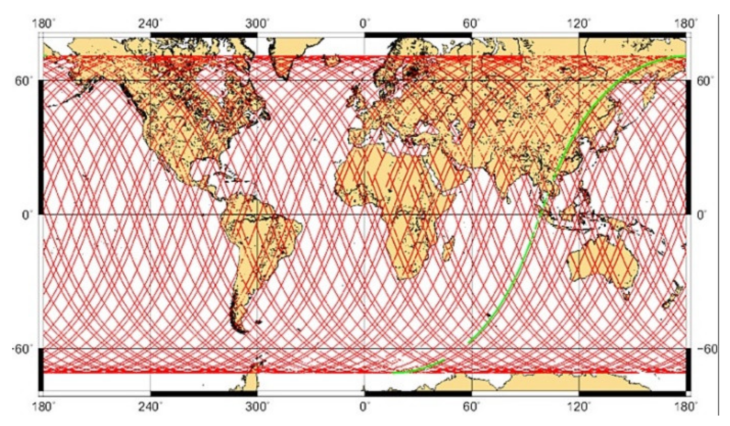
The region of modeling covers the main part of the Atlantic from Antarctica to 55° N. It includes the Caribbean Sea, the Sargasso Sea and the Gulf of Mexico, but excluding the Mediterranean Sea. The fixed values from the climatic Atlas [34] are set on the boundaries, and they do not change during the simulation interval. For data assimilation, we used the AVISO data of SLA along the satellite tracks, which are calculated by subtracting the values of sea level averaged over 10 years of observations (2002–2011) from the observed values of sea level.

The map with the tracks of the satellite that measures the sea-level data is shown in Figure 1.

On average, there are about 30,000 values of observed SLA, which is much smaller than the values 480 × 720 × 109~377 × 10⁷ produced per day by the model. Therefore, the model values were projected onto the observational points.

As a result of quality control, some observations of sea level were excluded from consideration, and about 10,000 values of ocean level for each day were used in DA; therefore, the dimension m of vector $Y_n$ is about 10,000. Then, the matrices in Equations (2), (5) and (6) used in the GKF method and those in Equations (2)–(4) used in the EnOI method have a dimension of ~ 10⁹.

3.2. Description of Numerical Experiments

The following DA experiments were carried out. Firstly, the spin-up run of the HYCOM model by atmospheric forcing, namely, wind and heat fluxes at the sea surface specified from the NCEP Reanalysis climatic atlas [35], was performed on a time interval of 40 model years. The results of calculations for each day over the last 10 years were stored and used further for constructing ensembles in the above-described data assimilation algorithms. Therefore, 109 model values at each grid point were recorded on each day from January 1 to December 31 for ten years.

Next, numerical experiments started on 1 January 2010 with the real 6-hourly wind and heat-flux forcing taken for this day from the GFS (Global Forecast System, NCEP) archive; they continued for a one-month time interval until January 31, 2010. Assimilation of SLA data was carried out according to Equations (2), (5) and (6) for GKF and (2)–(4) for EnOI. The information from the recorded results of modeling for each day for the last 10 years was used to calculate the characteristics of the anomaly matrix $Q_n$ according to Equation (8) and the trend $C_n$ according to Equation (5), for the assimilation time $t_n$ in chronological order from January 1 to January 31, 2010. As was already mentioned above, to use the GKF method correctly, the assimilation window must be much shorter than the total integration time. In these experiments, the total integration time is one month, much longer than the assimilation window, which is one day. The samples for the assimilation experiments were constructed as follows: for a day with number n, the data were chosen from the recorded archive for this day and for two days before and two days after this date with a time spacing of 2 days between them; altogether, 50 values were used. For example, to construct the sample for January 15, the data for January 11, 13, 15, 17 and 19 were used.

Three types of numerical experiments were executed: the control experiments with no data assimilation, those with DA by the GKF method and those with DA by the EnOI method. The initial and boundary conditions on the ocean–atmosphere interface were identical; the observational data and the ensemble dimensions were the same.

3.3. Results of Numerical Experiments and Their Analysis

To assess the quality of DA, we introduce the following variables. Let

$$va{r}_{m,n}=L^{-1}{\displaystyle \sum }_{i=1}^L{({(SL{A}_m)}_n^i-{(SL{A}_o)}_n^i)}^2$$

designate the error variance of the model with respect to the observations at time instant $t_n$; L is the total number of observations at time $t_n$;

$$va{r}_{f,n}=L^{-1}{{\displaystyle \sum }}_{i=1}^L{({(SL{A}_f)}_n^i-{(SL{A}_o)}_n^i)}^2,$$

$$va{r}_{a,n}=L^{-1}{{\displaystyle \sum }}_{i=1}^L{({(SL{A}_a)}_n^i-{(SL{A}_o)}_n^i)}^2,$$

are the forecast and analysis of model values of SLA, respectively, at time $t_n$ and at observation point i. The control model value is ${(SL{A}_m)}_n^i$. The forecast value ${(SL{A}_f)}_n^i$ designates the model forecast for time instant $t_n$ with the initial value known at the previous time instant $t_{n-1}$; the value of analysis ${(SL{A}_a)}_n^i$ is considered at the same time instant.

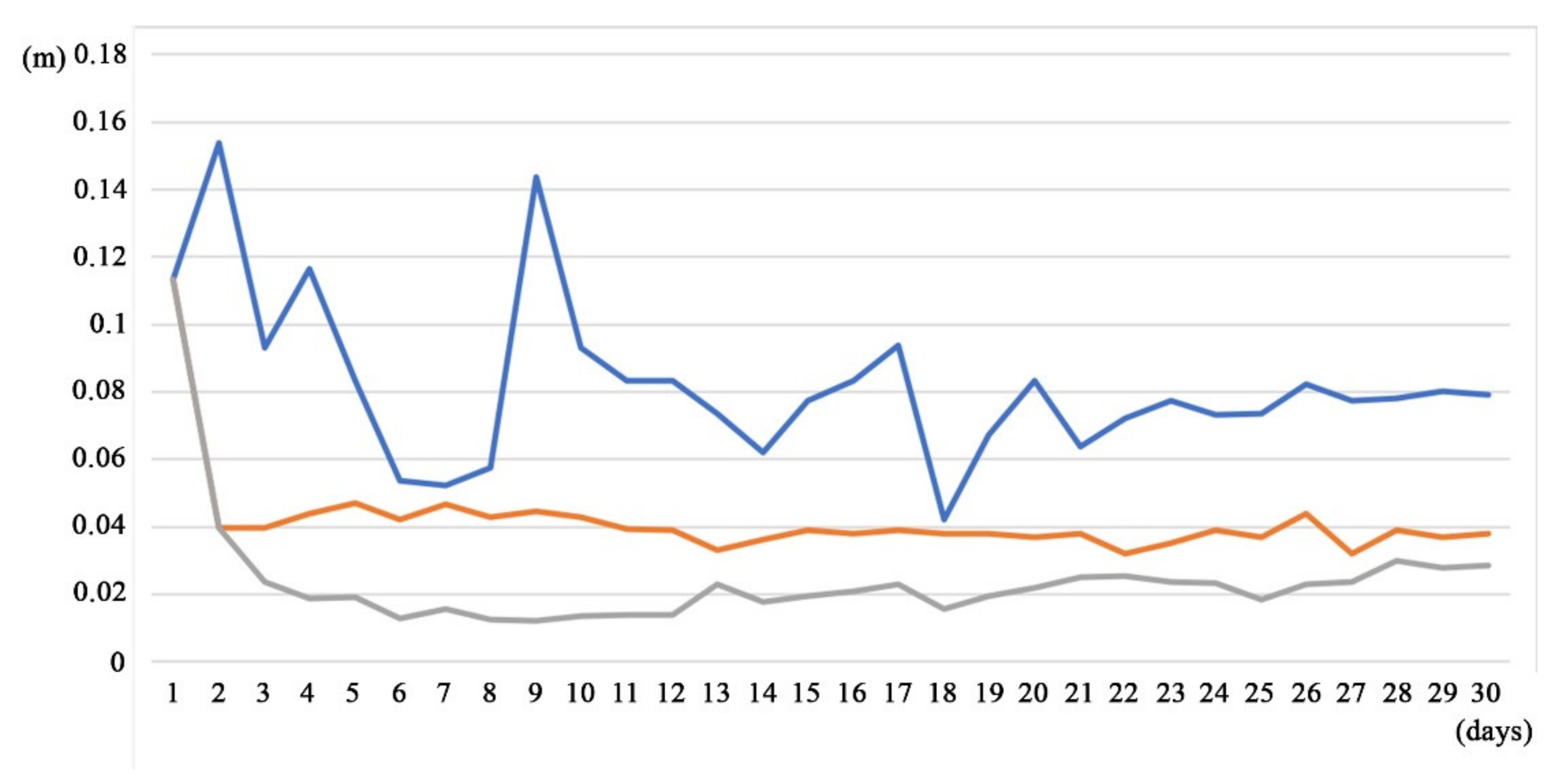
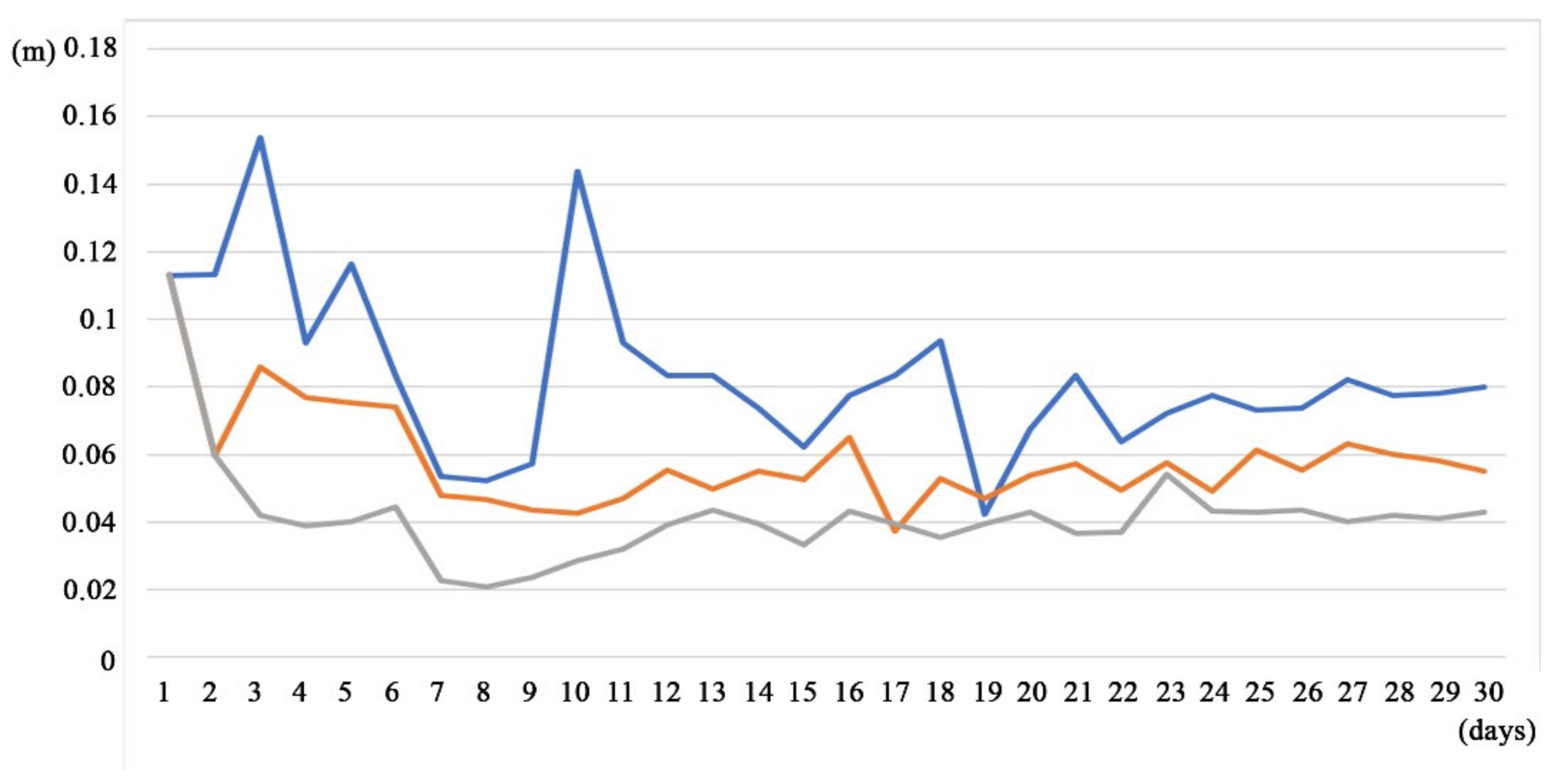
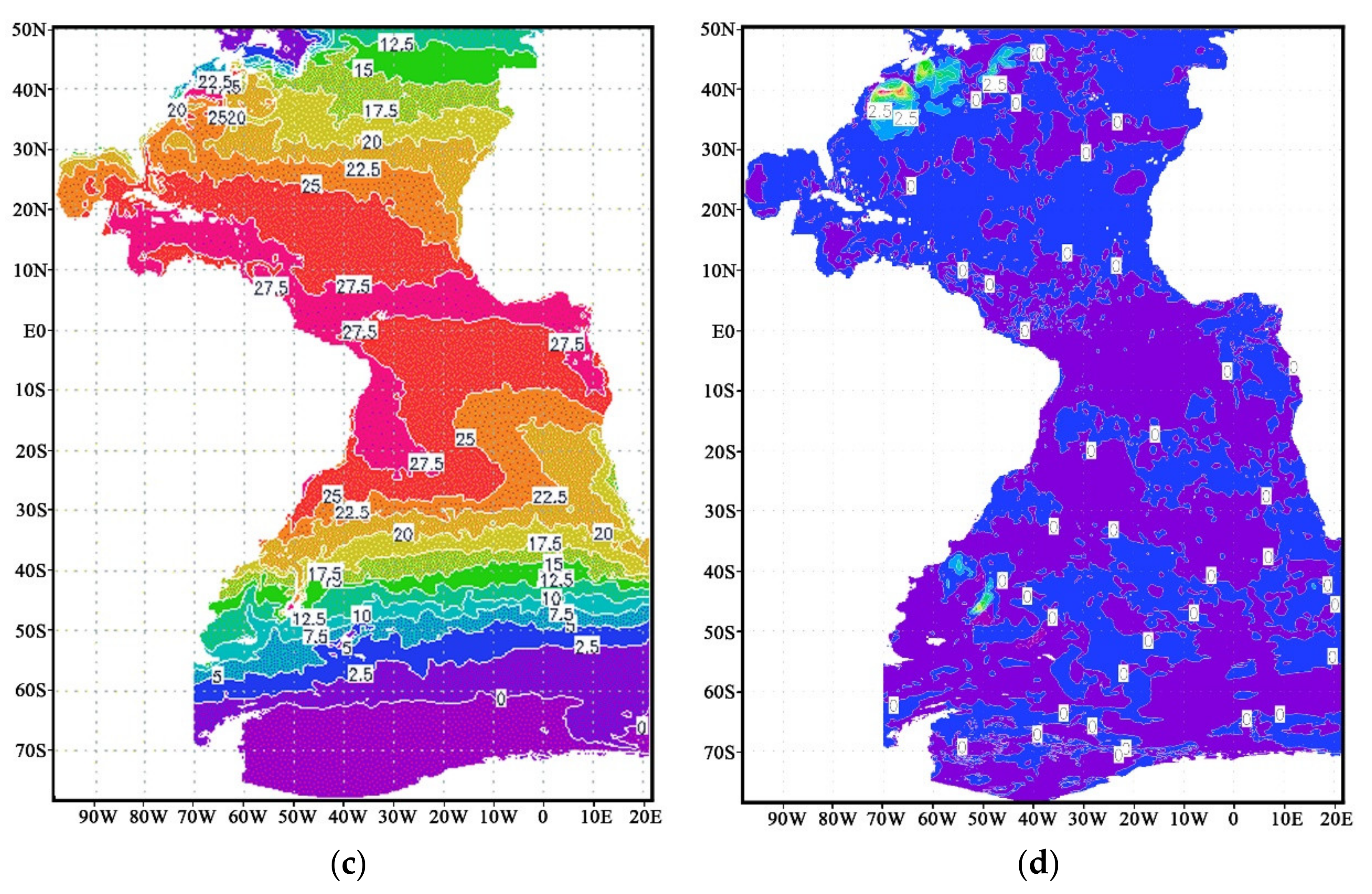
The timeline of the root mean square deviation of the square root of var_m,n, var_f,n and var_a,n are shown in Figure 2 and Figure 3. Figure 2 shows the analysis deviation; Figure 3 shows the 24-hour-forecast deviation. It is clear that the deviation of the control run for both experiments does not change.

As is seen from Figure 2 and Figure 3, the discrepancy between the results obtained by using the GKF and EnOI methods is observed only from the second day of calculation, since the calculation systems of equations for the GKF and EnOI methods for the first 24 h of calculation coincide with each other.

It is seen from Figure 2 and Figure 3 that the use of the GKF method has lower RMS errors in comparison with both calculations using the EnOI method and without DA (the control experiment). The forecast and analysis errors in the GKF method are much smaller: 0.5–0.3 of the control error and 0.5 of the error in the calculation using the EnOI method. We can also note that the EnOI method, in general, gives a smaller forecast error than the error of the control calculation; however, this is not true for the period around the 20th day. For the same period, the forecast error of the GKF method is always smaller than that of the control calculation and is nearly identical to the error of the EnOI method for 17 January 2010. The same conclusion can be made for the analysis error. However, it should be noted that both DA methods work correctly; they reduce the forecast error and improve the forecast capability of the model. We can also note that the control calculation gives a forecast error with a trend decreasing in time.

It is seen from Figure 2 and Figure 3 that the noticeable discrepancy between the results of calculations with the DA methods and the control calculation becomes stabilized by 27 January 2010; after this date, the calculated values of variances are nearly constant. Therefore, further analysis of the calculated fields and the data of independent observations is referred to this day.

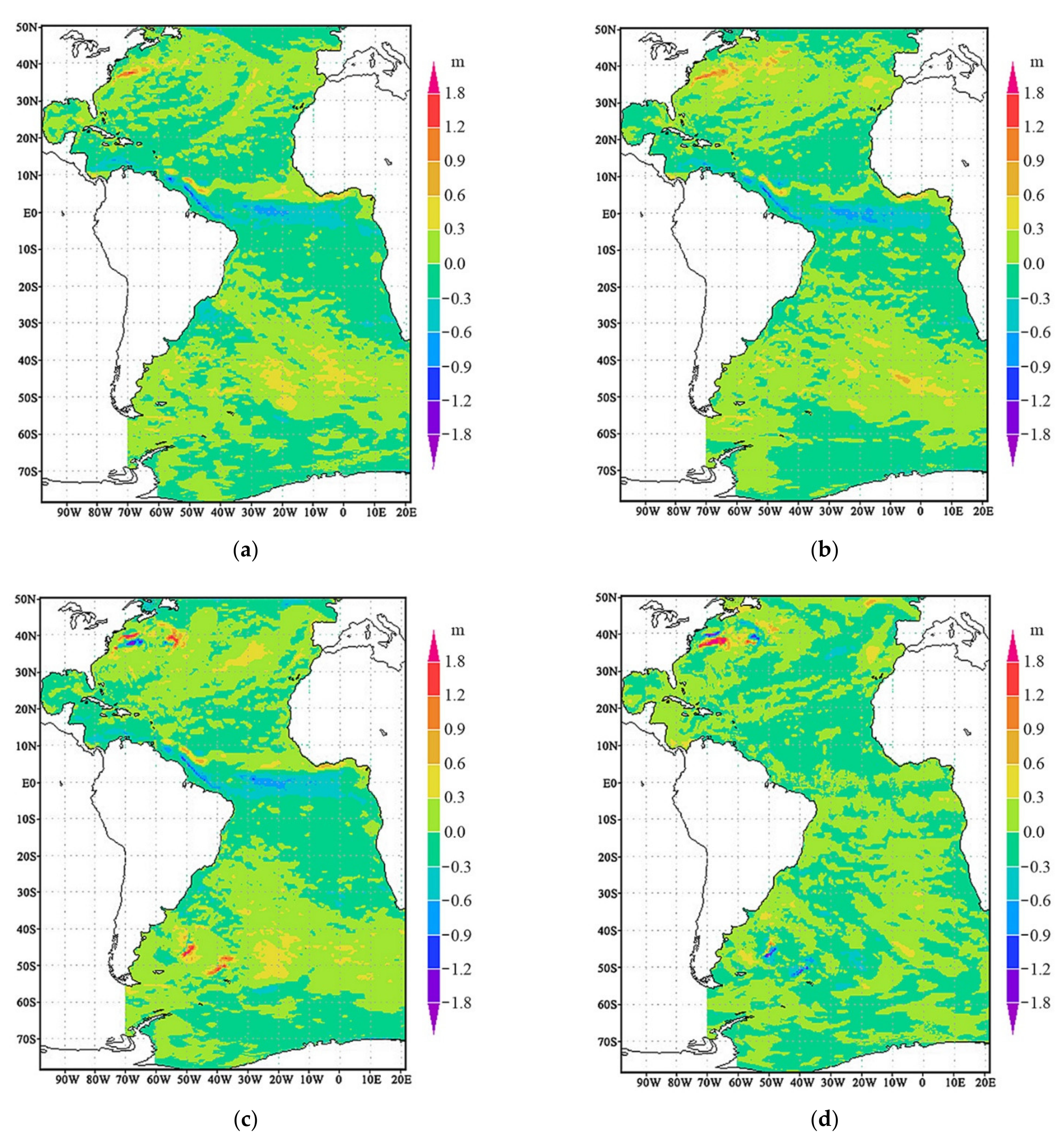
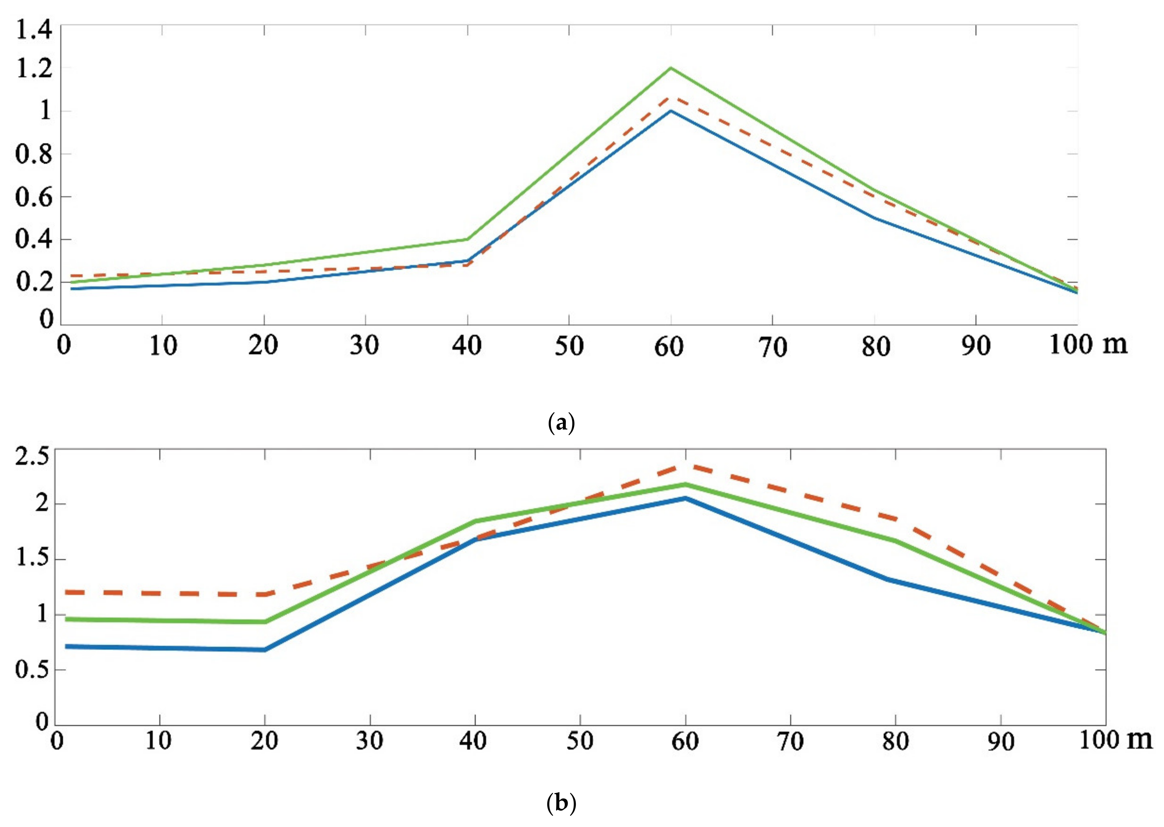
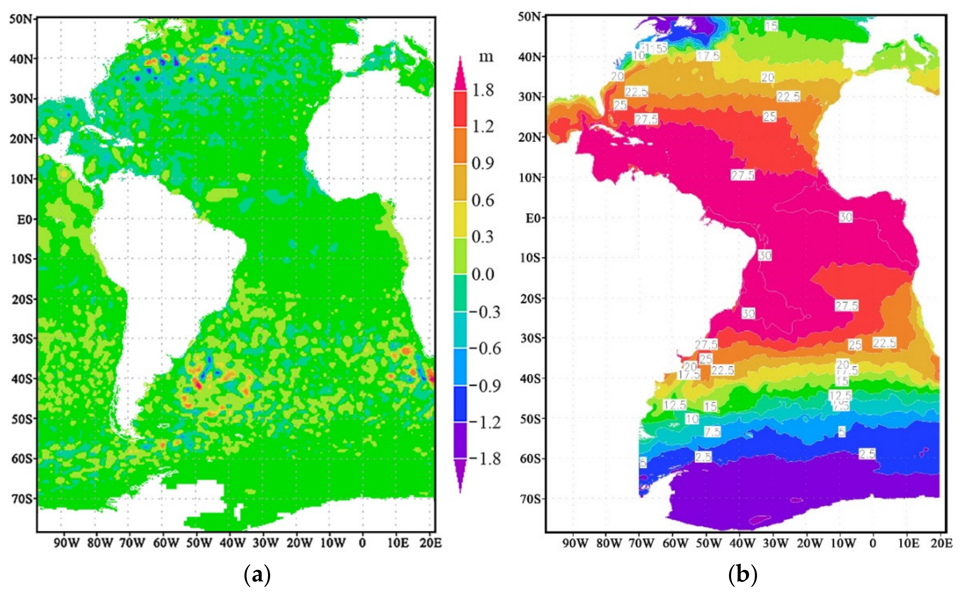
Figure 4 shows the values of modeled SLA fields. All figures are centered to zero, and green corresponds to zero, while red and blue show the deviation for positive and negative values, respectively.

All these figures show similar SLA structures in the Atlantic with some particular details. Figure 4a (control calculation) shows the general dynamical structure with strongly pronounced positive SLA values in the Gulf Stream zone and weakly expressed negative SLA values in the Brazil–Malvinas Confluence Zone in the South Atlantic. The negative zone of SLA is also clearly pronounced at the equator and extends along the coastal zone of South America in the Caribbean Sea and in the Gulf of Guinea.

The SLA field calculated by the EnOI method (Figure 4b) has the same structure; however, the positive anomalies in the Gulf Stream zone and the negative anomalies in the center of the Atlantic have close values but extend over a larger area. This can be explained by the fact that the EnOI method uses the ensemble statistics of 50 model calculations, the results of which may significantly vary. On the contrary, the GKF method makes the positive anomalies in the Gulf Stream significantly more pronounced and compact; at the same time, we can see a positive anomaly in the southern part of the Atlantic Ocean at 45° S, which corresponds to the synoptic state of SLA in this zone.

The difference between the SLA fields calculated by the EnOI and GKF methods (Figure 4d) confirms that this is a synoptic-scale effect. The positive anomaly appears neither in the control calculation nor in that using the EnOI method; however, it appears in the calculation by the GKF method. The same phenomenon is shown below when analyzing the real SLA trends.

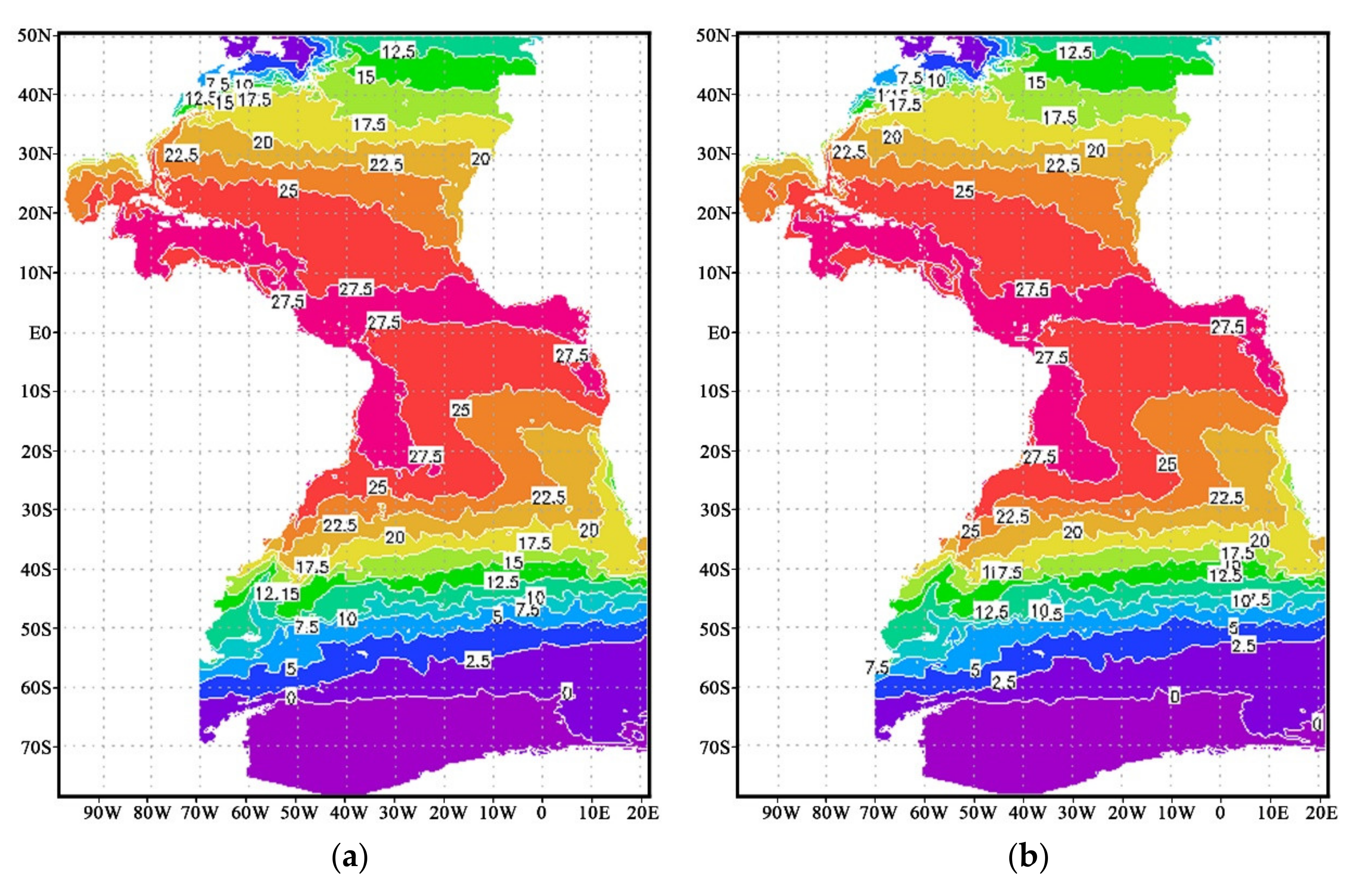
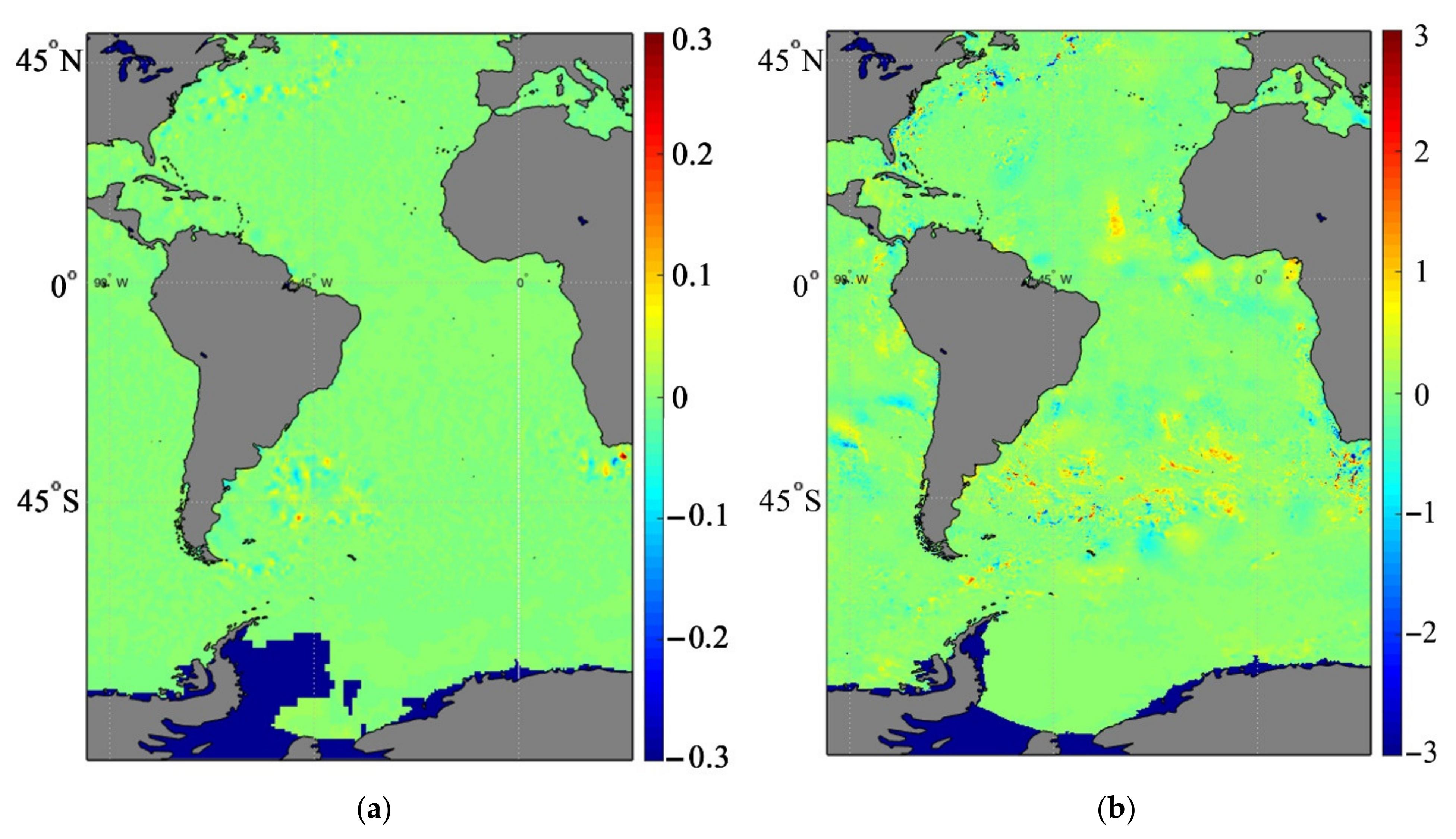
Figure 5 shows the results of calculations of Sea Surface Temperature (SST) for the same date, namely, on 27 January 2010: the control calculation (Figure 5a), the calculation with DA by the EnOI method (Figure 5b), the calculation with DA by the GKF method (Figure 5c), as well as the difference between the SST fields calculated by the EnOI and GKF methods (Figure 5d). No significant difference is seen between the SST fields of the control calculation (Figure 5a) and that using the EnOI method (Figure 5b); some difference is noticeable in the northern part of the Gulf Stream zone. Conversely, one can see a significant difference between the SST fields of the control calculation (Figure 5a) and that using the GKF method (Figure 5c), as well as the difference between the SST fields calculated by the EnOI and GKF methods (Figure 5d).

This difference is strongly pronounced in the northern region of the Atlantic, where a warm vortex appears and propagates along the current. This is a synoptic effect, and this meander is locally strongly pronounced. In the southern region of the Atlantic Ocean, near the Brazil–Malvinas Confluence Zone, local dynamics are also noticeable. We can also affirm that this is a synoptic effect associated with the variability in time, which is small in comparison with the total modeling time.

4. Comparison of the Results of Numerical Experiments with Independent Observational Data

4.1. Comparison with the Data from PIRATA Moorings

The results of three calculations of salinity and temperature using the HYCOM model, both with no data assimilation (the control calculation) and with data assimilation of the AVISO data using the EnOI and GKF methods, were compared with the independent observational data from the moored buoys of Pilot Research Array in the Tropical Atlantic (PIRATA) [36]. In the Tropical and Central Atlantic, there are 17 moored buoys that provide measurements of temperature and salinity from the sea surface down to a depth of 500 m. The map of PIRATA mooring locations can be seen on the website https://www.pmel.noaa.gov/gtmba/pirata-array-map (accessed on 21 July 2021). These daily data are freely available from http://pirata.ccst.inpe.br/en/data-2 (accessed on 21 July 2021).

To compare the results of all three calculations of salinity and temperature, they were interpolated independently of each other to the points of PIRATA buoys’ location separately for each depth level from the sea surface down to a depth of 500 m. In Figure 6a,b, the vertical axis presents the value of the difference between the model and observations (for salinity and temperature for the control and each assimilation method, respectively), and the horizontal axis presents the depth in meters. Figure 6a shows the deviation of the calculated salinity from the real PIRATA data. Figure 6b demonstrates the deviation of the calculated temperature from the PIRATA data. The green line refers to the difference between the results of the control calculation and the PIRATA data; the orange dashed line refers to the deviation of the results of calculation using the EnOI method from the PIRATA data; the blue line refers to the deviation of the results of calculation using the GKF method from the PIRATA data.

As it can be seen from Figure 6, the results of the calculation using the GKF method are closer to the observational data than the results of the control calculation and those obtained by the EnOI method. It is seen from Figure 6 that the largest discrepancy between the values of salinity and temperature calculated by all the methods, including the control calculation, from the real observational data is observed at 60 m depth. These curves are not shown for the depths below 100 m because the effect of assimilation of the SLA data at those depths is insignificant. The maximal deviations of both the calculated salinity and temperature from the observations occur below the upper quasi-homogeneous layer (the jump layer); the model cannot predict its exact position. However, the results of calculations with DA using both methods and those without DA are similar and describe the real surface and subsurface temperature and salinity.

4.2. Comparison with Independent SLA and SST Observations

Figure 7 shows the maps of satellite observations of the SLA (Figure 7a) and SST (Figure 7b) fields taken from the site ftp://podaac-ftp.jpl.nasa.gov/allData/ghrsst/data/L4/GLOB/UKMO/OSTIA/2010/ (accessed on 21 July 2021). Below we present the qualitative comparison of the results of model calculations with the observed SLA and SST fields.

The observed SLA field shown in Figure 7a is much more chaotic than the calculated SLA fields shown in Figure 4a–c; it contains numerous mesoscale eddies, strongly pronounced in the Gulf Stream and Brazil–Malvinas Confluence Zones. In the North–West Atlantic, the negative anomalies prevail, while in the South–West Atlantic, the positive anomalies are seen. The calculation using the GKF method (Figure 4c) reproduces this peculiarity better than the control calculation (Figure 4a) and the calculation using the EnOI method (Figure 4b).

The SST field presented in Figure 7b has all the features characteristic of the Central and South Atlantic, which are shown in Figure 5a–c. However, in Figure 7b, we can see mesoscale eddies in the Gulf Stream and Brazil–Malvinas Confluence Zones, while these eddies are seen neither in the control calculation (Figure 5a) nor in that using the EnOI method (Figure 5b). On the contrary, in the calculation using the GKF method (see Figure 5c), the well-pronounced eddies are seen in both the Gulf Stream and Brazil–Malvinas Confluence Zones, which agree very well with the observed SST. Therefore, we can assert that the results of calculation using the GKF method reproduce the synoptic variability in the ocean better than the results obtained by using the EnOI method and those without DA.

Figure 8a,b shows the daily changes of the observed values of SLA and SST on 27 January 2010, i.e., the differences between the values of SLA and SST observed on 27 January 2010 and those observed on 26 January 2010. The above-mentioned synoptic variability in the Gulf Stream and Brazil–Malvinas Confluence Zones is also clearly seen. Since these gradients are considered in the calculations of the sea level and temperature fields with DA using the GKF method (in Equation (8)), it is clear why the eddies are seen in Figure 4c and Figure 5c in the sea level and temperature fields and why the calculation using the GKF method has advantages over that using the EnOI method and the control calculation. The daily gradient of the observed SST field (Figure 8b) is very dynamic, has a pronounced vortex structure, with especially strongly pronounced dynamics in the northern region of the Atlantic.

5. Conclusions

In this study, the possibility of the practical application of the new Generalized Kalman Filter (GKF) DA method is shown; this method was compared with the Ensemble Optimal Interpolation (EnOI) method that is often used in practical applications. The advantages of the GKF method are shown. In particular, it provides a better 24 h forecast and gives a smaller error in a posteriori analysis. In addition, the GKF method reflects the ocean mesoscale variability and its dynamics better; the ocean salinity and temperature data calculated by the GKF method agree better with the independent PIRATA observations. The GKF and EnOI methods were compared because both of them have the same logical and methodological approach. However, in fact, the GKF method can be compared with any other DA method by using the same criteria for the identical dynamic model and data set for assimilation. For further validation and perfection of the GKF algorithm, we plan to apply this method with the Argo floats data [18].