Article

A Coupling between Integral Equations and On-Surface Radiation Conditions for Diffraction Problems by Non Convex Scatterers

by
Saleh Mousa Alzahrani
1,†,
Xavier Antoine
2,*,† and
Chokri Chniti
1,†
1
Department of Mathematics, University College in Al-Qunfudhah, Umm AlQura University, Al-Qunfudhah 28821, Saudi Arabia
2
Faculty of Science and Technology, Université de Lorraine, CNRS, Inria, IECL, F-54000 Nancy, France
*
Author to whom correspondence should be addressed.
These authors contributed equally to this work.
Mathematics 2021, 9(18), 2299; https://doi.org/10.3390/math9182299
Submission received: 15 August 2021 / Revised: 6 September 2021 / Accepted: 13 September 2021 / Published: 17 September 2021
(This article belongs to the Special Issue Numerical Analysis and Scientific Computing)

Abstract

:
The aim of this paper is to introduce an orignal coupling procedure between surface integral equation formulations and on-surface radiation condition (OSRC) methods for solving two-dimensional scattering problems for non convex structures. The key point is that the use of the OSRC introduces a sparse block in the surface operator representation of the wave field while the integral part leads to an improved accuracy of the OSRC method in the non convex part of the scattering structure. The procedure is given for both the Dirichlet and Neumann scattering problems. Some numerical simulations show the improvement induced by the coupling method.

1. Introduction

During the last decades, time-harmonic wave propagation has proved to be central in many engineering and technological key developments, based, e.g., on acoustics, electromagnetism or elastic mechanisms. When one wants to simulate the associated boundary-value problem, one of the difficulties is related to the fact that the solution which has to be computed is set in an exterior unbounded domain Ω + defined as the complementary of a finite scatterer Ω . Therefore, to use a standard numerical method, it is necessary to bound the computational domain. One well-known possibility is to use an absorbing boundary condition [1,2,3,4,5,6,7] or a Perfectly Matched Layer [8,9,10,11,12,13] to bound the domain and then solve the resulting problem by the finite element method [14,15,16]. Another widely used alternative is to rewrite equivalently the initial exterior PDE problem as an integral equation over the finite surface Γ of the scatterer Ω based on the Green’s function [17,18,19,20,21,22,23,24,25,26,27,28]. Then, this has the advantage of reducing from one the dimension of the problem. One of the main drawbacks is that, unlike the initial problem which involves partial differential operators, the integral equation is defined by construction as a nonlocal pseudodifferential operator. When a discretization technique is then applied, as the boundary element method, then the corresponding discrete version of the integral equation leads to the numerical solution of a highly indefinite complex-valued dense linear system which is particularly difficult to tackle in the high-frequency regime. Many technical aspects are then necessary to make it working correctly for some applications, for example to reduce the storage and to accelerate the solution of the linear system [17,18,29]. Various numerical methods were further developed to propose some other ways to solve, at least approximately, the initial scattering problem. One of them is the On-Surface Radiation Condition (OSRC) method introduced in [30] and further developed by many authors (see, e.g., [31]). Without giving too much details now, the OSRC approach also leads to solve an equation given over the surface of the scatterer, but defined through local surface partial differential operators. Therefore, after the application of the boundary element method, the linear system is highly sparse, yielding an efficient way to solve the scattering problem. The price to pay is that the method can be considered as a numerical asymptotic method, and therefore can lose some accuracy in some cases, in particular when the scatterer is not convex and includes some concave parts [31] where multiple scattering effects are present. Considering the problem of getting better accuracy for OSRC based techniques, a coupled formulation between the OSRC method and a two-dimensional finite element technique was proposed in [32] for scattering by single non convex obstacles. For the numerical simulation of multiple scattering problems (then leading to non convex global structures), coupled OSRC/integral equation formulations were presented in [33,34], where the shapes of the single obstacles are convex [33] or slightly non convex [34]. The aim of the present paper is to contribute to the improvement of the OSRC method for non convex single obstacles by proposing a direct simple coupling between the OSRC and the surface integral equation method. Unlike [32], the presented method is naturally only set on the boundary of the scatterer and does not suffer from the pollution error related to the finite element method.
The plan of the paper is the following: In Section 2, we introduce the two-dimensional Dirichlet scattering problem and the basic informations about the integral equation representations and their numerical approximation. Section 3 presents the notion of OSRC and its numerical discretization after writing the variational formulation. Section 4 develops the original coupling procedure for the Dirichlet problem. In particular, we explain how to formulate the problem and to improve its convergence properties if it is used in a Krylov solver, based on operator preconditioning. The coupling is validated in a simple two-dimensional example. The extension to the Neumann problem is shortly given in Section 5. Finally, Section 6 is a conclusion.

2. Two-Dimensional Scattering-Integral Equation Formulations

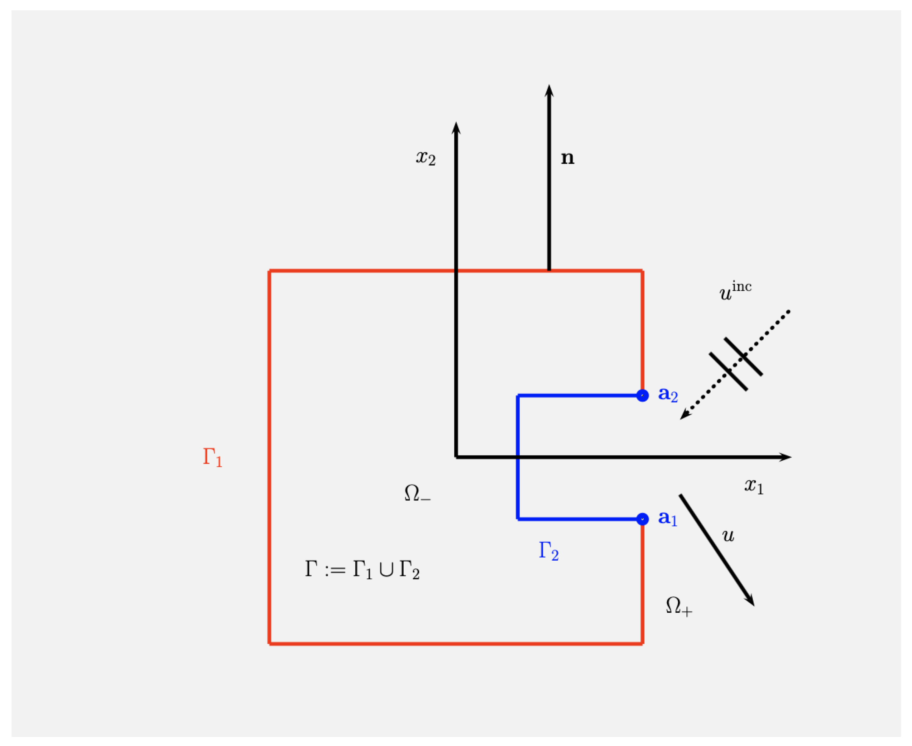
2.1. The Two-Dimensional Scattering Problem

Let us consider Ω as a scatterer with polygonal boundary Γ : = Ω . The homogeneous isotropic exterior domain of propagation is denoted by Ω + = R 2 \ Ω ¯ . For the sake of conciseness in the presentation, we first assume that the scatterer is acoustically sound-soft (i.e., Dirichlet boundary condition). Nevertheless, the case of a sound-hard scattering problem (Neumann boundary condition) is also treated shortly in Section 5. We now consider a time-harmonic incident plane wave u inc ( x ) = e i k θ inc · x (with x = ( x 1 , x 2 ) R 2 ) illuminating Ω , with an incidence direction θ inc = ( cos ( θ inc ) , sin ( θ inc ) ) for a time dependence e i ω t , setting ω as the wave pulsation and k as the wavenumber. The sound-soft scattering problem of u inc by Ω leads to the computation of the scattered wavefield u C 2 ( Ω + ) C 0 ( Ω + ¯ ) as the solution to the boundary-value problem
( Δ + k 2 ) u = 0 , in Ω + , u = u inc , on Γ , lim | | x | | + | | x | | 1 / 2 ( u · x | | x | | i k u ) = 0 .
We designate by ( Δ + k 2 ) the Helmholtz operator, where Δ = x 1 2 + x 2 2 is the laplacian. The gradient operator is ∇ and | | x | | = x · x , where x · y is the scalar product of two vectors x and y of R 2 . The last equation of (1) is the well-known Sommerfeld’s radiation condition at infinity that ensures the uniqueness of the scattered wave field u. The outwardly directed unit normal vector to Ω is n . A schematic representation of the problem is given in Figure 1. The existence and uniqueness of the solution to this BVP is well-known and detailed in [20], Theorem 2.12. From standard arguments connecting formulations in classical and Sobolev spaces ([20], p. 107), then u H loc 1 ( Ω + ) and u is C up to Γ , excluding the corners of the polygonal curves ([20], Lemma 2.35). Following [20], Theorem 2.12, then it can also be proved that u n L 2 ( Γ ) .

2.2. Integral Operators for Scattering

Let us define G as the two-dimensional free-space Green’s kernel
x , y R 2 , x y , G ( x , y ) = i 4 H 0 ( 1 ) ( k x y ) ,
where H 0 ( 1 ) is the first-kind Hankel’s function of order zero. Building an integral equation needs the Helmholtz integral representation formula ([20], Theorems 2.20 and 2.21).
Proposition 1. 
If v C 2 ( Ω + ) H loc 1 ( Ω + ) is a solution to the Helmholtz equation in an unbounded domain Ω + which also satisfies the Sommerfeld radiation condition, then the following relation holds
Γ G ( x , y ) n v ( y ) + n y G ( x , y ) v ( y ) d Γ ( y ) = v ( x ) if x Ω + , 0 otherwise .
In addition, let us assume that v C 2 ( Ω ) H 1 ( Ω ) is solution to the Helmholtz equation in a bounded domain Ω . One can write
Γ G ( x , y ) n v ( y ) + n y G ( x , y ) v ( y ) d Γ ( y ) = 0 if x Ω + , v ( x ) otherwise .
Let us now introduce the volume single- and double-layer integral operators, respectively, denoted by L and M , that are defined for ρ L 2 ( Γ ) by
x R 2 \ Γ , L : ρ L ρ ( x ) = Γ G ( x , y ) ρ ( y ) d Γ ( y ) , x R 2 \ Γ , M : ρ M ρ ( x ) = Γ n y G ( x , y ) ρ ( y ) d Γ ( y ) .
The wave fields v and v (see (3) and (4)) can be expressed as
v ( x ) = L ( n v | Γ ) ( x ) M ( v | Γ ) ( x ) , x Ω + , v ( x ) = L ( n v | Γ ) ( x ) + M ( v | Γ ) ( x ) , x Ω .
Furthermore, the single- and double-layer integral operators provide some outgoing solutions to the Helmholtz equation [20].

2.3. Direct Boundary Integral Equations for the Dirichlet Problem

The aim of this section is to provide without any detail the standard integral equation formulations for solving the two-dimensional scattering problem with Dirichlet boundary condition that will be used later. More details can be found in [17,20,28] for the derivation and properties of these integral equations (well-posedness, existence of resonant modes,...). Let us introduce the following boundary integral operators
L ρ ( x ) = Γ G ( x , y ) ρ ( y ) d Γ ( y ) , M ρ ( x ) = Γ n y G ( x , y ) ρ ( y ) d Γ ( y ) , N ρ ( x ) = Γ n x G ( x , y ) ρ ( y ) d Γ ( y ) , D ρ ( x ) = n x Γ n y G ( x , y ) ρ ( y ) d Γ ( y ) .
Then, based on the expressions of the trace and normal derivative trace of the volume single- and double-layer potentials (see, e.g., [20] for further details), a first formulation is based on the trace of the single-layer operator
L ρ = u inc | Γ in L 2 ( Γ ) ,
where the unknown density ρ is an element of L 2 ( Γ ) . The equation is well-posed and equivalent to the exterior scattering problem (1) as soon as k is not an irregular interior frequency of the associated Dirichlet boundary-value problem [17,20,28]. This integral equation is called Electric Field Integral Equation (EFIE) in electromagnetism. In the sequel, this formulation will be denoted by Single-Layer Integral Equation (SLIE). In the case of a closed boundary Γ , which is the situation in the paper, it can be proved that the spurious internal modes do not radiate. Therefore, there is no pollution in the far-field computation, which justifies that the SLIE can be considered as a reference solution. In addition, for an open surface Γ , the SLIE is the only possible integral equation that can be written.
Another surface integral formulation is given by (see [20] for the functional framework associated to the integral equations)
( 1 2 I + N ) ρ = n u inc | Γ .
It is also well-posed and equivalent to the exterior scattering problem (1) if k is not an interior Neumann resonance [17,28]. This formulation is often designated by Magnetic Field Integral Equation (MFIE). Nevertheless, this integral equation is not recommended in practice since the spurious modes radiate and introduce some errors when computing the far-field pattern. To avoid the interior resonance problem, Burton and Miller [17,19,28] proposed to rather use a linear combination between the EFIE and MFIE. If α is a real-valued parameter such that 0 < δ < 1 and if η is a complex parameter with ( η ) 0 , where ( η ) is the imaginary part of η , then one gets the Combined Field Integral Equation (CFIE) [17,23,28] or Burton-Miller Integral Equation (BWIE)
( 1 δ ) ( 1 2 I + N ) + δ η L ρ = ( 1 δ ) n u inc | Γ δ η u inc | Γ .
This integral equation is well-posed for any wavenumber k but can only be applied to closed surfaces.
An important point is that all these integral equations are based on the single-layer representation
x Ω + , u ( x ) = L ρ ( x ) ,
where the unknown surface field ρ is the physical quantity defined by the jump (set as the difference between the interior and exterior traces)
ρ = [ n u ] Γ : = n u | Γ + + n u | Γ = ( n u | Γ + n u | Γ inc ) .
To compute the far-field pattern, let us recall that we have: u = L ρ + M λ , where ρ and λ are two unknown densities. In the polar coordinates system ( r , θ ) , the use of asymptotic expansions when r + leads to the following relation [22]
θ [ 0 , 2 π ] , u ( r , θ ) = e i k r r 1 / 2 a L ( θ ) + a M ( θ ) + O 1 r 3 / 2 ,
where a L and a M are the radiated far-fields for the single- and double-layer potentials, respectively, defined for any angle θ of [ 0 , 2 π ] by
a L ( θ ) = 1 8 k π e i π / 4 Γ e i k θ · y ρ ( y ) d Γ ( y ) , a M ( θ ) = 1 8 k π e i π / 4 Γ i k y θ · y e i k θ · y λ ( y ) d Γ ( y ) ,
with θ : = ( cos ( θ ) , sin ( θ ) ) . In addition, the Sonar Cross Section (SCS) (in dB ) is such that
θ [ 0 , 2 π ] , σ ( θ ) = 10 log 10 ( 2 π a L ( θ ) + a M ( θ ) 2 ) .
When using the single-layer representation (9), only a L is needed while a M is set to zero. In the paper, we will focus on the SLIE.

2.4. Numerical Approximation

To numerically solve Equation (6) (or (8)), we first introduce a polygonal interpolating surface Γ h which approximates Γ . The triangularization of Γ h is built by using n K linear segments K j of size h. Therefore, we have Γ h = j = 1 n K K j . In the numerical examples, we take about 10 elements per wavelength which is enough to get a suitable accuracy for the Boundary Element Method (BEM). The notation P designates the space of complex-valued polynomials of order . In (6) (or (8)), no derivative operator is applied to the unknown ρ . However, as seen below, the OSRC method, and the integral equation technique for the Neumann problems introduce some tangential derivatives that apply to the surface fields. For this reason, we propose to use the linear BEM all along the paper, where the conformal finite element space V h of P 1 piecewise continuous functions is defined by
V h : = ϕ h C 0 ( Γ h ) ; ϕ K j : = ϕ h K j P 1 , j = 1 , . . . , n K .
For the Dirichlet problem, a P 0 (constant per segment) BEM could also be applied. For the numerical approximation, we naturally use the weak form of the integral Equation (6) which leads to [27]
q L 2 ( Γ ) , Γ Γ G ( x , y ) ρ ( y ) q ( x ) d Γ ( y ) d Γ ( x ) = Γ u inc | Γ ( x ) q ( x ) d Γ ( x ) .
Let us consider now that the BEM is applied. To compute the elementary interaction
I ( K 1 , K 2 ) : = K 1 K 2 G ( x , y ) d K 2 ( y ) d K 1 ( x ) ,
for two segments K 1 and K 2 of Γ h , a standard semi-analytical integration formula is used. This means that there is a first outer integration in (13) according to x on K 1 and based on a two-points Gauss–Legendre quadrature. Next, for the inner integral with respect to y on K 2 , if K 1 K 2 , then again a two-points Gauss–Legendre quadrature is applied, an exact integration formula is used [35] when K 1 = K 2 . By using the interpolating surface Γ h and the linear approximations of both ρ and q in V h , the discrete form of (12) yields the linear system
L ρ = M u inc ,
where L is the complex-valued matrix associated with the single-layer operator and M is the surface mass matrix. If n P is the number of points of the curve Γ h , then all the matrices are elements of the space M n P ( C ) of complex-valued matrices of size n P × n P . Indeed, assuming that Γ is a closed boundary, then the number of degrees of freedom of the linear boundary element method, i.e., the number of points n P : = dim ( V h ) , is equal to the number of segments: n P = n K . In addition, the unknown complex-valued nodal vector ρ and the nodal incident vector u inc are in C n P . For computing the coefficients of L , some semi-analytical quadrature formula are used to integrate the kernel singularity. If one rather uses the BWIE (8), the discrete form leads to
[ ( 1 δ ) ( 1 2 M + N ) + δ η V ) ] ρ = ( 1 δ ) M n u inc δ η M u inc ,
where n u inc is the nodal complex-valued vector related to the normal trace of the incident field. Finally, we have
ρ = ( n u + n u inc ) .

3. Loss of Accuracy of the OSRC Method for Non Convex Scatterers

3.1. First and Second-Order OSRCs

The on-surface radiation condition (OSRC) method was introduced in the middle of the eighties by Kriegsmann, Taflove and Umashankar [30]. At that time, the main idea was to develop an approximate but efficient and low memory numerical solution for scattering problems, most particularly in the high-frequency regime. Starting from local approximations of the Dirichlet-to-Neumann (DtN) operator, they were able to propose the computation of the scattered field by two-dimensional simple obstacles. Since then, the OSRC method has received much attention from many researchers and many improvements and extensions have been proposed (see, e.g., [31]). For the sake of conciseness, we restrict our presentation to the so-called first- and second-order Bayliss–Turkel-like radiation conditions [36].
The first-order OSRC (that we denote by OSRC 1 ) is given by
n u 1 + ( i k + κ 2 ) u 1 = 0 , on Γ .
In the above equation, ( u 1 , n u 1 ) is the OSRC Cauchy data that approximate the exact Cauchy data ( u , n u ) on Γ . Here, let us remark that ( u 1 , n u 1 ) must be understood as a notation since the OSRC is an approximate DtN map, which means that we do not a priori know if n u 1 is the normal derivative trace of a function u 1 . The function κ : = κ ( s ) is the curvature at a point s of the surface, where s is the curvilinear abscissa counterclockwise directed along Γ . Equation (17) can be seen as a simple impedance boundary condition for the exterior domain Ω + . Various ways of deriving (17) are available in the literature. Let us mention for example [1] were formal and rigorous approaches are developed.
The first-order OSRC (17) can be improved, leading to the so-called symmetrical second-order Bayliss–Turkel condition (denoted by OSRC 2 in the sequel)
n u 2 + ( i k + κ 2 κ 2 8 ( κ i k ) ) u 2 s ( 1 2 ( κ i k ) s ) u 2 = 0 , on Γ .
In (18), the curvilinear derivative operator is written s u = u · τ , where τ is the tangent vector to Γ ( n · τ = 0 ). In the same spirit, an Engquist–Majda-like OSRC can be derived [1,31]. However, some numerical simulations in various papers show that the boundary condition (18) provides a higher accuracy. Therefore, in the present paper, we restrict our study to (18).

3.2. Numerical Approximation

To solve (18), we introduce the weak formulation
Γ n u 2 v d Γ + Γ ( i k + κ 2 κ 2 8 ( κ i k ) ) u 2 v d Γ + Γ 1 2 ( κ i k ) s u 2 s v d Γ = 0 , on Γ ,
for some suitable test-functions v in H 1 ( Γ ) . The pair of approximate Cauchy data ( u 2 , n u 2 ) is discretized in the finite element space V h × V h . When the BEM is introduced, then the discretization of (19) can be rewritten at the matrix level as
M n u 2 + ( M β + S α ) u 2 = 0 ,
where the functions α and β are defined for OSRC 2 by
α = 1 2 ( κ i k ) , β = i k + κ 2 κ 2 8 ( κ i k ) .
The matrices S α and M β are, respectively, the (sparse) n P × n P generalized stiffness and mass matrices associated with the functions α and β . In addition, the vectors u 2 and n u 2 are complex-valued vector fields of C n K . Finally, the second-order OSRC method requires the following stable approximation scheme for the curvature [36]: let K = ( a 1 a 2 a 3 ) be a triangle whose vertices a j , j = 1 , 2 , 3 , are points on Γ h , then, the curvature at the vertex a 2 can be approximated by
κ ( a 2 ) = 4 × area ( K ) a 1 a 2 a 3 ,
where a j , for j = 1 , , 3 , are the lengths of the edges of K ordered with respect to the increasing size. This formula is directly applied on the triangles associated with the surface mesh and built on two adjacent segments. Using Formula (21) implies that the curvature is not equal to zero at the corner of the square since the triangle used to compute the numerical curvature is not flat. For a uniform surface mesh with size h, the numerical curvature is given as 2 / h . This allows us to reproduce the scattering phenomenon arising at the corner (see also [36]).
Since we are solving a scattering problem with given Dirichlet boundary condition, then u 2 is given by u inc and then
M n u 2 = ( M β + S h α ) u inc .
This means that n u 2 is simply obtained through the solution of a complex-valued sparse linear system defined by the mass matrix. Once the unknown is obtained then one can compute an approximation of the jump of the normal derivative trace by the relation
ρ 2 = ( n u 2 + n u inc ) .
Another way of writing this relation is that ρ 2 is solution to
M ρ 2 = ( M β 2 + S h α 2 ) u inc M n u inc : = g 2 .
The far-field can be directly obtained through expressions (11).
Even if the boundary condition (17) can be a priori applied to any scatterer Ω , we will see during the numerical simulations that a serious loss of accuracy is observed when the scatterer presents some concave parts (see [36] and Figure 1, Figure 2 and Figure 3). Indeed, in the concavity, the presence of multiply bounced rays cannot be modeled by local differential operators since the nature of this phenomena is nonlocal. Therefore, the aim of the next sections is to provide an original way to directly couple the OSRC formulation in the convex part of the scatterer to the SLIE restricted to the concave part to improve the accuracy.

4. The Coupling Procedure for Non Convex Scatterers

4.1. Weak Coupling Procedure and Boundary Element Approximation

Since the OSRC solution is locally inaccurate in the non convex part of the domain, we propose to build a solution which is computed first by the OSRC method and improved thanks to the integral equation where the quality of the OSRC approximation deteriorates. To this end, let us assume that the geometry Γ can be decomposed into two non-overlapping parts Γ : = Γ 1 Γ 2 , with Γ 1 Γ 2 = a 1 ; a 2 . The geometry Γ 1 is related to the boundary part of Γ which is convex, the complementary (where we will use an integral equation) is Γ 2 (see Figure 1). The proposed procedure uses 1) a global computation of an approximate surface density ρ 2 through the OSRC on Γ and 2) injects the restriction of this approximation to Γ 1 into the global integral equation formulation on Γ to obtain an approximate density on Γ 2 . This way of partitioning the computation allows us to solve a smaller size boundary element system and can be seen as a ”one shot” computation.
In the following, if A is a global matrix on Γ , we denote by A j the extracted matrix related to the interaction between the part Γ j of the boundary and Γ , j , = 1 , 2 . We then have
A = A 11 A 12 A 21 A 22 .
In a similar way, the restriction of a nodal complex-valued vector z to the part of the boundary Γ is written z , for = 1 , 2 . Then, we propose the following algorithm for the SLIE formulation: compute ρ 2 : = ( ρ 1 2 , ρ ˜ 2 2 ) C n P such that
( 1 ) OSRC : extract ρ 1 2 = ( ρ 2 ) 1 C n P 1 2 from the computation of M ρ 2 = g 2 , ( 2 ) SLIE : compute ρ ˜ 2 2 C n P 2 as the solution to L 22 ρ ˜ 2 2 = L 21 ρ 1 2 ( M u inc ) 2 .
Even if other coupling possibilities are available, this one has the advantage that no modification of an existing code is required. Let us denote by n K j (respectively, n P j ) the number of segments (respectively, points) of the boundary Γ j , j = 1 , 2 , based on the uniform mesh used for the full BEM on Γ h . Then, we have n K = n K 1 + n K 2 and n P = n P 1 + n P 2 2 (the two junction points a 1 and a 2 must be counted once). In step 1), we only retain the values of the OSRC solution that are not considered in the cavity, including the two endpoints a 1 and a 2 . This first step needs O ( n K ) operations to solve the sparse complex-valued linear system (by using an LU factorization or a preconditioned iterative Krylov solver [37]) while the memory storage is O ( n K 1 ) . In the second step, the solution to a complex-valued full matrix is necessary. If a full storage is considered, then the linear system solution needs O ( n K 2 3 ) elementary operations and the memory storage is O ( n K 2 2 ) . Usually, in integral equation solvers, most particularly for high-frequency scattering, it is preferable to use a subspace Krylov solver [17,37,38] in conjunction with a fast matrix-vector product algorithm like for example the Multilevel Fast Multipole Method (FMM) [24], high-order solvers [18] or the recent direct Adaptive Cross Approximation (ACA) techniques [29]. In this case, the memory requirement is O ( n K 2 ) for a computational cost O ( n K 2 log n K 2 ) . In addition, it is well-known that preconditioning is a requirement to get a fast convergence. The second equation of (26) is defined through the single-layer integral operator. Then, the integral equation is a first-kind Fredholm equation which is known to be badly conditioned. To improve this, we propose a preconditioned version of the algorithm (26) based on the Caldèron relations [17] and well-adapted to fast iterative solvers but without modifying the solution of the initial coupling procedure. Let D be the discrete version of the normal derivative trace operator D and D 22 its restriction to Γ 2 . Then, the preconditioned version of (26) is given by: find ρ 2 : = ( ρ 1 2 , ρ ˜ 2 2 ) C n P such that
( 1 ) compute ρ 1 2 = ( ρ 2 ) 1 C n P 1 2 solution to M ρ 2 = g 2 , ( 2 ) obtain ρ ˜ 2 2 C n P 2 as the solution to D 22 L 22 ρ ˜ 2 2 = D 22 L 21 ρ 1 2 D 22 ( M u inc ) 2 .
The second equation of (27) is defined by a second-kind integral equation formulation which has better clustering properties for the convergence of Krylov subspace solvers. The price to pay is that each iteration of a Krylov solver requires to apply L 22 first and next D 22 . The preconditioned Caldèron SLIE coupling procedure (27) is called SLIE-OSRC 2 . Once ρ ˜ 2 : = ( ρ 1 2 , ρ ˜ 2 2 ) C n P has been computed, all the usual quantities of interest can be obtained like for the SCS given by (11).
The SLIE-OSRC 2 formulation may suffer from the existence of interior resonances. Even if the spurious modes do not radiate for the SLIE, it can be better to have access to a stable formulation. To this end, the following BWIE-OSRC 2 coupling procedure could alternatively be used: compute ρ ˜ 2 : = ( ρ 1 2 , ρ ˜ 2 2 ) C n P such that
( 1 ) ρ 1 2 = ( ρ 2 ) 1 C n P 1 2 is solution to M ρ 2 = g 2 , ( 2 ) extract ρ ˜ 2 2 C n P 2 from the solution to [ ( 1 δ ) ( 1 2 M 22 + N 22 ) + δ η V 22 ) ] ρ ˜ 2 2 = [ ( 1 δ ) ( 1 2 M 21 + N 21 ) + δ η V 21 ) ] ρ 1 2 ( 1 δ ) ( M n u inc ) 22 δ η ( M u inc ) 22 .
Unlike the SLIE-OSRC 2 formulation, the BWIE-OSRC 2 approach is defined by a second-kind Fredholm integral equation and does not really need to be preconditioned when correctly choosing δ and η (see, e.g., [17]). An extra computational cost and memory storage is required since the evaluation of the double-layer potentials N 22 and N 21 are required.
In the following examples, we will report only the results related to the SLIE-OSRC 2 formulation since no resonance were met and we always plot the SCS. In addition, we do not use any iterative solver for the resulting linear systems because we are considering toys problems for a proof of concept. However, for three-dimensional problems, where the method directly extends, the difference between all the formulations may be important in terms of convergence rate. Here, we rather focus on the accuracy improvement. Further investigations are therefore needed, as well as improved formulations and implementation of higher order OSRCs.

4.2. A Numerical Example-Validation of the Procedure

As previously said, we use the SLIE-OSRC 2 formulation. The model toy problem is the following. We consider the obstacle Ω as being composed of the square cylinder centered at the origin and with side length 2, with an inner square cavity defined by the corners ( 1 / 3 , 1 / 3 ) , ( 1 , 1 / 3 ) , ( 1 , 1 / 3 ) and ( 1 / 3 , 1 / 3 ) . The boundary Γ 2 is then defined as the internal boundary to the cavity (blue curve on Figure 1) and Γ 1 is the complementary boundary on Γ (red curve on Figure 1). For an incident plane wave, the reference solution is given by the SLIE (14) discretized by the BEM (with 10 points per wavelength). The results are clearly improved compared to the pure OSRC approach for wave numbers k 15 and this, independently of the angle of attack θ inc . As it can be observed on the first picture of Figure 2 (Case 1, for k = 2 ), we almost obtain the reference solution by using the SLIE-OSRC 2 approach while a pure OSRC approximation gives a poor accuracy which deteriorates as k increases. For a higher wave number (Case 2, k = 8 ), the results are still accurate (see Figure 2). By increasing the frequency, we still have an acceptable solution as seen on the third example of Figure 2 (Case 3, k = 14 ). For both the integral equations and OSRCs, since we consider a mesh with ten elements per wavelength, the size of the matrix L 2 , 2 is about n K 2 = 2.5 k , which is more than four times less than for a pure SLIE solution.

5. The Neumann Scattering Problem

The Neumann scattering problem, i.e., considering (1) but with the boundary condition: n u = n u inc on Γ , can be treated similarly with the EFIE [17] based on the normal derivative trace of the double-layer potential written under its weak form (called DLIE). A hyper-singular kernel must then be integrated carefully by semi-integration techniques. For the OSRC, the method applies quite similarly and leads to the solution of a sparse linear system.
In general, the coupling procedure (called DLIE-OSRC 2 ) has proved to be less accurate than for the Dirichlet problem (i.e., for SLIE-OSRC 2 ). We think that this is due to the fact that the OSRC approach requires a higher order operator to provide a suitable fast solution during the first step of the method. We recommend to rather use the square-root OSRC developed in [2]. The resulting coupling technique will be analyzed in a forthcoming work. For low and moderate wave numbers ( k 4 ), we still get quite acceptable results having always in mind the lower computational cost of the DLIE-OSRC 2 method. However, there is a moderate accuracy for wave numbers such that k 10 as seen on the two cases reported in Figure 3. Nevertheless, this must be counterbalanced by the lower cost of the procedure and the possibility to increase the OSRC accuracy in the convex part. In addition, we always obtain a good prediction of the main lobs where the energy is mostly radiating. As a general concluding remark, the coupling DLIE-OSRC 2 algorithm provides an interesting alternative to the DLIE. Furthermore, the method is always more accurate than a classical OSRC approach and gives a possibility of its extension to non-convex obstacles.

6. Conclusions

In this paper, we introduced a simple and original algorithm coupling the surface integral equation method and the OSRC technique for solving the scattering problem by nonconvex scatterers. While simple, the coupling method leads to an improved accuracy compared with the pure OSRC approach and reduces the computational cost of a direct integral equation formulation. In addition, we explain how operator preconditioning can be directly included into the formulations. The method is validated on a simple two-dimensional problem as a proof of concept. In particular, the method is accurate for the Dirichlet problem, but still needs to be further investigated by using high-order OSRCs in the case of the Neumann problem. We expect that the formulation can be useful for three-dimensional high-frequency scattering problems solved iteratively by Krylov solvers with acceleration algorithms.

Author Contributions

Conceptualization, software, formal analysis, investigation, writing—original draft preparation, writing—review and editing, S.M.A., X.A. and C.C.; project administration, funding acquisition, S.M.A. and C.C. All authors have read and agreed to the published version of the manuscript.

Funding

The authors would like to thank the Deanship of Scientific Research at Umm Al-Qura University for supporting this work by Grant code 18-SCI-1-01-0017.

Informed Consent Statement

Not applicable.

Conflicts of Interest

The authors declare no conflict of interest.

Abbreviations

The following abbreviations are used in this manuscript:
OSRCOn-Surface Radiation Condition
EFIEElectric Field Integral Equation
SLIESingle-Layer Integral Equation
MFIEMagnetic Field Integral Equation
CFIECombined Field Integral Equation
BWIEBurton-Miller Integral Equation
SCSSonar Cross Section
BEMBoundary Element Method
DtNDirichlet-to-Neumann
DLIEDouble-Layer Integral Equation

References

  1. Antoine, X.; Barucq, H.; Bendali, A. Bayliss-Turkel-like Radiation Condition on Surfaces of Arbitrary Shape. J. Math. Anal. Appl. 1999, 229, 184–211. [Google Scholar] [CrossRef]
  2. Antoine, X.; Darbas, M.; Lu, Y. An Improved Surface Radiation Condition for High-Frequency Acoustic Scattering Problems. Comput. Methods Appl. Mech. Eng. 2006, 195, 4060–4074. [Google Scholar] [CrossRef]
  3. Givoli, D. High-order local non-reflecting boundary conditions: A review. Wave Motion 2004, 39, 319–326. [Google Scholar] [CrossRef]
  4. Hagstrom, T. Radiation boundary conditions for the numerical simulation of waves. Acta Numer. 1999, 8, 47–106. [Google Scholar] [CrossRef]
  5. Hagstrom, T.; Warburton, T. A new auxiliary variable formulation of high-order local radiation boundary conditions: Corner compatibility conditions and extensions to first-order systems. Wave Motion 2004, 39, 327–338. [Google Scholar] [CrossRef]
  6. Modave, A.; Geuzaine, C.; Antoine, X. Corner treatments for high-order local absorbing boundary conditions in high-frequency acoustic scattering. J. Comput. Phys. 2020, 401, 109029. [Google Scholar] [CrossRef] [Green Version]
  7. Tsynkov, S. Numerical solution of problems on unbounded domains. A review. Appl. Numer. Math. 1998, 27, 465–532. [Google Scholar] [CrossRef]
  8. Bérenger, J.P. A perfectly matched layer for the absorption of electromagnetic waves. J. Comput. Phys. 1994, 114, 185–200. [Google Scholar] [CrossRef]
  9. Bérenger, J.P. Perfectly matched layer (PML) for computational electromagnetics. Synth. Lect. Comput. Electromagn. 2007, 2, 1–117. [Google Scholar] [CrossRef] [Green Version]
  10. Bermúdez, A.; Hervella-Nieto, L.; Prieto, A.; Rodríguez, R. Perfectly matched layers. In Computational Acoustics of Noise Propagation in Fluids-Finite and Boundary Element Methods; Springer: Berlin/Heidelberg, Germany, 2008; pp. 167–196. [Google Scholar]
  11. Bermúdez, A.; Hervella-Nieto, L.; Prieto, A.; Rodríguez, R. Perfectly matched layers for time-harmonic second order elliptic problems. Arch. Comput. Methods Eng. 2010, 17, 77–107. [Google Scholar] [CrossRef] [Green Version]
  12. Druskin, V.; Güttel, S.; Knizhnerman, L. Near-optimal perfectly matched layers for indefinite Helmholtz problems. SIAM Rev. 2016, 58, 90–116. [Google Scholar] [CrossRef] [Green Version]
  13. Turkel, E.; Yefet, A. Absorbing PML boundary layers for wave-like equations. Appl. Numer. Math. 1998, 27, 533. [Google Scholar] [CrossRef]
  14. Bériot, H.; Prinn, A.; Gabard, G. Efficient implementation of high-order finite elements for Helmholtz problems. Int. J. Numer. Methods Eng. 2016, 106, 213–240. [Google Scholar] [CrossRef] [Green Version]
  15. Ihlenburg, F. Finite Element Analysis of Acoustic Scattering; Number 132 in Applied Mathematical Sciences; Springer: New York, NY, USA, 1998. [Google Scholar]
  16. Solin, P.; Segeth, K.; Dolezel, I. Higher-Order Finite Element Methods; CRC Press: Boca Raton, FL, USA, 2003. [Google Scholar]
  17. Antoine, X.; Darbas, M. An Introduction to Operator Preconditioning for the Fast Iterative Integral Equation Solution of Time-Harmonic Scattering Problems. Multiscale Sci. Eng. 2021, 1, 1–35. [Google Scholar] [CrossRef]
  18. Antoine, X.; Geuzaine, C.; Ramdani, K. Wave Propagation in Periodic Media-Analysis, Numerical Techniques and Practical Applications; Progress in Computational Physics; Chapter Computational Methods for Multiple Scattering at High Frequency with Applications to Periodic Structures Calculations; Bentham Books: Sharjah, United Arab Emirates, 2010; Volume 1, pp. 73–107. [Google Scholar]
  19. Burton, A.J.; Miller, G.F. The application of integral equation methods to the numerical solution of some exterior boundary-value problems. Proc. R. Soc. Lond. A Math. Phys. Sci. 1971, 323, 201–210. [Google Scholar]
  20. Chandler-Wilde, S.; Graham, I.; Langdon, S.; Spece, E. Numerical-asymptotic boundary integral methods in high-frequency acoustic scattering. Acta Numer. 2012, 21, 89–305. [Google Scholar] [CrossRef] [Green Version]
  21. Colton, D.; Kress, R. Inverse Acoustic and Electromagnetic Scattering Theory, 2nd ed.; Applied Mathematical Sciences; Springer: Berlin, Germany, 1998; Volume 93. [Google Scholar]
  22. Colton, D.L.; Kress, R. Integral Equation Methods in Scattering Theory; Pure and Applied Mathematics (New York); John Wiley & Sons Inc.: New York, NY, USA, 1983. [Google Scholar]
  23. Harrington, R.; Mautz, J. H-field, E-field and combined field solution for conducting bodies of revolution. Arch. Elektron. Uebertragungstechnik 1978, 4, 157–164. [Google Scholar]
  24. Liu, Y. Fast Multipole Boundary Element Method: Theory and Applications in Engineering; Cambridge University Press: Cambridge, UK, 2009. [Google Scholar]
  25. Martin, P.A. Multiple Scattering. Interaction of Time-Harmonic Waves with N Obstacles; Encyclopedia of Mathematics and its Applications; Cambridge University Press: Cambridge, UK, 2006; Volume 107, p. xii+437. [Google Scholar]
  26. McLean, W. Strongly Elliptic Systems and Boundary Integral Equations; Cambridge University Press: Cambridge, UK, 2000. [Google Scholar]
  27. Nédélec, J.C. Acoustic and Electromagnetic Equations. Integral Representations for Harmonic Problems; Applied Mathematical Sciences; Springer: New York, NY, USA, 2001; Volume 144. [Google Scholar]
  28. Thierry, B. Analyse et Simulations Numériques du Retournement Temporel et de la Diffraction Multiple. Ph.D. Thesis, Nancy University, Nancy, France, 2011. [Google Scholar]
  29. Hackbusch, W. Hierarchical Matrices: Algorithms and Analysis; Springer: Berlin/Heidelberg, Germany, 2015; Volume 49. [Google Scholar]
  30. Kriegsmann, G.; Taflove, A.; Umashankar, K. A new formulation of electromagnetic wave scattering using an on-surface radiation boundary condition approach. IEEE Trans. Antennas Propag. 1987, 35, 153–161. [Google Scholar] [CrossRef]
  31. Antoine, X. Computational Methods for Acoustics Problems; Chapter Advances in the On-Surface Radiation Condition Method: Theory, Numerics and Applications; Saxe-Coburg Publications: Stirling, UK, 2008; pp. 169–194. [Google Scholar]
  32. Antoine, X. An algorithm coupling the OSRC and FEM for the computation of an approximate scattered acoustic field by a non-convex body. Int. J. Numer. Methods Eng. 2002, 54, 1021–1041. [Google Scholar] [CrossRef]
  33. Alzubaidi, H.; Antoine, X.; Chniti, C. Formulation and accuracy of On-Surface Radiation Conditions for acoustic multiple scattering problems. Appl. Math. Comput. 2016, 277, 82–100. [Google Scholar] [CrossRef] [Green Version]
  34. Acosta, S. On-surface radiation condition for multiple scattering of waves. Comput. Methods Appl. Mech. Eng. 2015, 283, 1296–1309. [Google Scholar] [CrossRef] [Green Version]
  35. Sauter, S.; Schwab, C. Boundary Element Methods; Springer Series in Computational Mathematics; Springer: Berlin/Heidelberg, Germany, 2011. [Google Scholar]
  36. Antoine, X. Fast Approximate Computation of a Time-Harmonic Scattered Field using the On-Surface Radiation Condition Method. IMA J. Appl. Math. 2001, 66, 83–110. [Google Scholar] [CrossRef]
  37. Saad, Y. Iterative Methods for Sparse Linear Systems; PWS Publishing Company: Boston, MA, USA, 1996. [Google Scholar]
  38. Saad, Y.; Schultz, M. GMRES: A Generalized Minimal Residual algorithm for solving nonsymmetric linear systems. SIAM J. Sci. Stat. Comput. 1986, 7, 856–869. [Google Scholar] [CrossRef] [Green Version]
Figure 1. Scattering configuration and notations.
Mathematics 09 02299 g001
Figure 2. Bistatic SCS for the unit square cylinder with cavity and Dirichlet boundary condition: Case 1:  k = 2 and θ inc = 135 deg., Case 2:  k = 8 and θ inc = 160 deg. and Case 3:  k = 14 and θ inc = 150 deg.
Mathematics 09 02299 g002
Figure 3. Bistatic SCS for the unit square cylinder with cavity and Neumann boundary condition: Case 1:  k = 9 and θ inc = 140 deg.; Case 2:  k = 13 and θ inc = 160 deg.
Mathematics 09 02299 g003
Publisher’s Note: MDPI stays neutral with regard to jurisdictional claims in published maps and institutional affiliations.

