Asymptotic Phase and Amplitude for Classical and Semiclassical Stochastic Oscillators via Koopman Operator Theory

Abstract

The asymptotic phase is a fundamental quantity for the analysis of deterministic limit-cycle oscillators, and generalized definitions of the asymptotic phase for stochastic oscillators have also been proposed. In this article, we show that the asymptotic phase and also amplitude can be defined for classical and semiclassical stochastic oscillators in a natural and unified manner by using the eigenfunctions of the Koopman operator of the system. We show that the proposed definition gives appropriate values of the phase and amplitude for strongly stochastic limit-cycle oscillators, excitable systems undergoing noise-induced oscillations, and also for quantum limit-cycle oscillators in the semiclassical regime.

1. Introduction

Spontaneous rhythmic oscillations and synchronization are widely observed in various fields of science and technology [1,2,3,4,5,6]. Regular rhythmic oscillations are generally modeled by using nonlinear dynamical systems possessing stable limit-cycle attractors.

The notion of asymptotic phase [1,2,3,4,5], which increases with a constant frequency in the basin of the limit-cycle attractor, is a fundamental quantity that provides a basis for phase reduction [1,2,3,4,5,6,7], a standard dimensionality-reduction method for analyzing synchronization of limit-cycle oscillators under the effect of weak perturbation or coupling.

Recently, the asymptotic phase and isochrons (level sets of the asymptotic phase), classical notions in the theory of nonlinear oscillations since Winfree [8] and Guckenheimer [9], have been studied from a viewpoint of the Koopman operator theory by Mauroy, Mezić, and Moehlis [10], and their relationship with the Koopman eigenfunction associated with the fundamental frequency of the oscillator has been clarified [10,11,12,13,14]. Moreover, they have shown that the (asymptotic) amplitude and isostables, which characterize deviation of the system state from the limit cycle and extend the Floquet coordinates [13,15,16] to the nonlinear regime, can be introduced naturally in terms of the Koopman eigenfunctions associated with the Floquet exponents with non-zero real parts [10,11,12,13,14,17]. By using the asymptotic phase and amplitude functions, we can obtain a reduced description of limit-cycle oscillators, which is useful for the analysis and control of synchronization dynamics of limit-cycle oscillators [18,19,20,21,22,23,24]. The theory can also be generalized to delay-differential systems [25] and spatially extended systems [26].

How to generalize the definition of the conventional asymptotic phase, which was essentially deterministic [8,9], to stochastic systems has been an intriguing problem [27,28,29,30,31,32,33,34,35,36]. When the stochasticity is sufficiently weak, the phase and also amplitude can be defined by using the drift term of the stochastic differential equation (SDE) describing the deterministic vector field of the oscillator. This approach can also be employed for quantum nonlinear oscillators in the semiclassical regime described by a quantum Fokker–Planck equation (FPE) [33,37]. However, this definition is no longer applicable to strongly stochastic oscillatory systems for which the deterministic vector field does not serve as a clear reference due to the strong effect of noise.

To cope with this problem, Schwabedal and Pikovsky [34] introduced a definition of the phase in terms of the mean first return time, and Thomas and Lindner [35] proposed a definition of the asymptotic phase in terms of the slowest decaying eigenfunction of the backward Fokker–Planck (Kolmogorov) operator describing the mean first passage time, both of which yield phase values that increase with a constant frequency on average for stochastic oscillations in a similar way to the ordinary asymptotic phase for deterministic oscillators. Recently, we pointed out that the definition of the stochastic asymptotic phase by Thomas and Lindner [35] can be seen as a natural extension of the deterministic definition from the viewpoint of the Koopman operator theory; namely, it is given by the argument of the Koopman eigenfunction associated with the fundamental frequency [38] (see also Reference [39]) and extended this idea to the definition of the asymptotic phase for quantum oscillatory systems.

In this article, based on the Koopman operator theory for stochastic systems, we propose a definition of the asymptotic phase and amplitude for strongly stochastic oscillators. They are introduced in terms of the eigenfunctions of the Koopman operator associated with the complex eigenvalues with the largest non-zero real part and with the largest non-zero real eigenvalue, respectively, which gives a natural extension of the definition in the deterministic case. The validity of the proposed definition is illustrated for stochastic limit-cycle oscillations and noise-induced oscillations of excitable systems using noisy Stuart–Landau [2,4] and FitzHugh–Nagumo [40,41] models as examples. Moreover, we apply the proposed definition of the stochastic phase and amplitude to a quantum limit-cycle oscillator in the semiclassical regime and show that they also yield appropriate results.

2. Phase and Amplitude for Deterministic Limit-Cycle Oscillators

2.1. Classical Definition of the Asymptotic Phase and Amplitude

In this section, we review the definition of the asymptotic phase and amplitude for deterministic limit-cycle oscillators and discuss their relationship with the Koopman eigenfunctions [10,11,12,13,14,19,26]. We consider a deterministic dynamical system

$$\begin{array}{c}\hfill \dot{\mathit{X}}\left(t\right)=\mathit{A}\left(\mathit{X}\left(t\right)\right),\end{array}$$

(1)

where $\mathit{X}\left(t\right)\in {\mathbb{R}}^N$ is the system state at time t, $\mathit{A}:{\mathbb{R}}^N\to {\mathbb{R}}^N$ is a sufficiently smooth vector field representing the system dynamics, and the dot $\left(\dot{}\right)$ represents the time derivative. We assume that the system has an exponentially stable limit-cycle solution ${\mathit{X}}_0\left(t\right)$ with a natural period T and frequency $\omega =2\pi /T$, satisfying ${\mathit{X}}_0(t+T)={\mathit{X}}_0\left(t\right)$. We denote this limit cycle as $\chi$ and its basin of attraction as $B_{\chi }\subseteq {\mathbb{R}}^N$. Instead of the time t, we can parameterize a point on the limit cycle $\chi$ using a phase $\varphi \in [0,2\pi )$ as $\mathbf{\chi }\left(\varphi \right)={\mathit{X}}_0\left(\omega t\right)$ ($0\le t<T$), where the phase value $\varphi =\omega t$ increases linearly with time t from 0 to $2\pi$ ($2\pi$ is identified with 0), and the origin of the phase $\varphi =0$ is assigned to the state ${\mathit{X}}_0\left(0\right)$ without loss of generality.

The linear stability of $\chi$ is characterized by the Floquet exponents ${\lambda }_j\in \mathbb{C}$ ($j=0,1,\dots ,N-1$) [15,42], which we sort in decreasing order of their real parts, i.e., $\mathrm{Re}\left({\lambda }_0\right)\ge \mathrm{Re}\left({\lambda }_1\right)\ge \mathrm{Re}\left({\lambda }_2\right)\ge \cdots \ge \mathrm{Re}\left({\lambda }_{N-1}\right)$. Here, the exponent ${\lambda }_0$ is zero and associated with the phase direction tangent to $\chi$, and the other exponents ${\lambda }_1,\dots ,{\lambda }_{N-1}$ possess negative real parts because $\chi$ is exponentially stable and is associated with the amplitude directions deviating from $\chi$. We further assume that ${\lambda }_1$ is real and ${\lambda }_1\gg \mathrm{Re}\left({\lambda }_2\right)$, namely, the relaxation of the slowest decaying mode is non-oscillatory and much slower than the other faster decaying modes. Such a situation often occurs in realistic models of limit-cycle oscillators. We can then focus only on the slowest decaying mode and introduce a single real amplitude associated with it.

The asymptotic phase function ${\Phi }_0:B_{\chi }\to [0,2\pi )$ and amplitude function $R_0:B_{\chi }\to \mathbb{R}$ of the limit cycle $\chi$ are defined in the basin $B_{\chi }$ of $\chi$ such that

$$\begin{array}{cc}\hfill \mathit{A}\left(\mathit{X}\right)·\nabla {\Phi }_0\left(\mathit{X}\right)& =\omega ,\hfill \\ \hfill \mathit{A}\left(\mathit{X}\right)·\nabla R_0\left(\mathit{X}\right)& ={\lambda }_1{R}_0\left(\mathit{X}\right),\hfill \end{array}$$

(2)

are satisfied for all $\mathit{X}\in B_{\chi }$ [13]. Here, the inner product is defined as $\mathit{a}·\mathit{b}={\sum }_{j=1}^N\overline{a_j}{b}_j$ (the overline denotes complex conjugate) and $\nabla =\partial /\partial \mathit{X}$ represents the gradient with respect to $\mathit{X}$. As stated above, we focus only on the phase associated with ${\lambda }_0=0$ and the slowest decaying amplitude associated with real ${\lambda }_1$. In general, we can introduce $N-1$ amplitude variables associated with $N-1$ exponents ${\lambda }_1,\dots ,{\lambda }_{N-1}$, which are in general complex, and obtain a closed set of equations for the phase and amplitudes [13]. The level sets of the phase function are called isochrons [8,9] and those of the amplitude function are called isostables [10].

By using the above definition, we can introduce the phase and amplitude variables for the oscillator state $\mathit{X}\left(t\right)\in B_{\chi }$ at time t as $\varphi \left(t\right)={\Phi }_0\left(\mathit{X}\left(t\right)\right)$ and $r\left(t\right)=R_0\left(\mathit{X}\left(t\right)\right)$, which obey

$$\begin{array}{cc}\hfill \dot{\varphi }\left(t\right)={\dot{\Phi }}_0\left(\mathit{X}\left(t\right)\right)& =\mathit{A}\left(\mathit{X}\left(t\right)\right)·\nabla {\Phi }_0\left(\mathit{X}\left(t\right)\right)=\omega ,\hfill \\ \hfill \dot{r}\left(t\right)={\dot{R}}_0\left(\mathit{X}\left(t\right)\right)& =\mathit{A}\left(\mathit{X}\left(t\right)\right)·\nabla R_0\left(\mathit{X}\left(t\right)\right)={\lambda }_1{R}_0\left(\mathit{X}\right)={\lambda }_{1}r\left(t\right),\hfill \end{array}$$

(3)

that is, the phase $\varphi$ always increases with a constant frequency $\omega$ and the amplitude r decays exponentially with the rate ${\lambda }_1$ as $\mathit{X}$ evolves in $B_{\chi }$ toward $\chi$.

Note that the phase function is determined only up to an arbitrary constant and the scale of the amplitude function $R_0\left(\mathit{X}\right)$ is also arbitrary, because ${\Phi }_0\left(\mathit{X}\right)+c_1$ and $c_2{R}_0\left(\mathit{X}\right)$ with arbitrary constants $c_1,c_2\in \mathbb{R}$ also satisfy Equation (2). Suppose that the initial state is ${\mathit{X}}_0\in B_{\chi }$ at $t=0$. If we assign the phase $\varphi (0;{\mathit{X}}_0)$ and amplitude $r(0;{\mathit{X}}_0)$ to the initial state ${\mathit{X}}_0$, we obtain $\varphi (t;{\mathit{X}}_0)=\omega t+\varphi (0;{\mathit{X}}_0)$ and $r(t;{\mathit{X}}_0)=r(0;{\mathit{X}}_0)exp\left({\lambda }_{1}t\right)$, whose dependence on ${\mathit{X}}_0$ is explicitly shown.

By focusing only on the asymptotic phase and amplitude, we can perform phase-amplitude reduction (or isochron-isostable reduction) of a limit-cycle oscillator [12,14,18,19], in which we reduce the dimensionality of the system dynamics from N to 2 and approximately describe it by a simple set of two-dimensional phase and amplitude equations. The phase equation has been extensively used for the analysis of weakly coupled limit-cycle oscillators [1,2,3,4,5,6], and the amplitude equation has also been used recently for the analysis and control of limit-cycle oscillators [18,19,20,21,24].

2.2. Koopman Operator Viewpoint

The asymptotic phase and amplitude introduced in the previous subsection are closely related to the Koopman operator of the system [18,19,20,21]. The Koopman operator $U^{\tau }$, which describes the evolution of a general observable g of the system state $\mathit{X}\in {\mathbb{R}}^N$, is defined as

$$\begin{array}{c}\hfill \left(U^{\tau }g\right)\left(\mathit{X}\right)=g\left(S^{\tau }\mathit{X}\right),\end{array}$$

(4)

where $g:{\mathbb{R}}^N\to \mathbb{C}$ is the observable, i.e., an observation function that maps a system state to an observed value, and $S^{\tau }:{\mathbb{R}}^N\to {\mathbb{R}}^N$ is a flow of the system satisfying $\mathit{X}(t+\tau )=S^{\tau }\mathit{X}\left(t\right)$ for $\tau \ge 0$. When the flow $S^{\tau }$ is analytic, it can be expanded as

$$\begin{array}{c}\hfill S^{\tau }\mathit{X}=\mathit{X}+\tau \mathit{A}\left(\mathit{X}\right)+O\left({\tau }^2\right)\end{array}$$

(5)

for $\left|\tau \right|\ll 1$. Considering an analytic observable g, we can expand it as

$$\begin{array}{c}\hfill g\left(S^{\tau }\mathit{X}\right)=g\left(\mathit{X}\right)+\tau \mathit{A}\left(\mathit{X}\right)·\nabla g\left(\mathit{X}\right)+O\left({\tau }^2\right).\end{array}$$

(6)

Therefore, the infinitesimal time evolution of g can be expressed as

$$\begin{array}{c}\hfill \frac{d}{dt}g\left(\mathit{X}\right)=\underset{\tau \to 0}{lim}\frac{U^{\tau }g\left(\mathit{X}\right)-g\left(\mathit{X}\right)}{\tau }=\underset{\tau \to 0}{lim}\frac{g\left(S^{\tau }\mathit{X}\right)-g\left(\mathit{X}\right)}{\tau }=\mathit{A}\left(\mathit{X}\right)·\nabla g\left(\mathit{X}\right).\end{array}$$

(7)

The operator

$$\begin{array}{c}\hfill A=\mathit{A}\left(\mathit{X}\right)·\nabla ,\end{array}$$

(8)

which appeared in Equation (3), can thus be interpreted as an infinitesimal generator of the Koopman operator $U^{\tau }$.

For the limit-cycle oscillator described by Equation (1), we can easily confirm that the complex exponential of the phase function ${\Phi }_0\left(\mathit{X}\right)$,

$$\begin{array}{c}\hfill {\Psi }_0\left(\mathit{X}\right)=e^{i{\Phi }_0\left(\mathit{X}\right)},\end{array}$$

(9)

is an eigenfunction of the operator A with an eigenvalue $i{\omega }_1$ where $i=\sqrt{-1}$, because

$$\begin{array}{c}\hfill A{\Psi }_0\left(\mathit{X}\right)=i\omega {\Psi }_0\left(\mathit{X}\right)\end{array}$$

(10)

is satisfied for $\mathit{X}\in B_{\chi }$. Therefore, from the viewpoint of the Koopman operator theory, the asymptotic phase can be introduced as the argument (polar angle) of the Koopman eigenfunction ${\Psi }_0\left(\mathit{X}\right)$ associated with the eigenvalue $i\omega$, which is determined by the natural frequency $\omega$ of the oscillator [18,19,20,21], as

$$\begin{array}{c}\hfill {\Phi }_0\left(\mathit{X}\right)=\mathrm{Arg}{\Psi }_0\left(\mathit{X}\right),\end{array}$$

(11)

where $\mathrm{Arg}$ represents the principal argument of a complex number in the range $[0,2\pi )$. Moreover, the asymptotic amplitude function $R_0\left(\mathit{X}\right)$ is nothing but the eigenfunction of the linear operator A associated with the eigenvalue ${\lambda }_1$ for $\mathit{X}\in B_{\chi }$, i.e.,

$$\begin{array}{c}\hfill A{R}_0\left(\mathit{X}\right)={\lambda }_1{R}_0\left(\mathit{X}\right).\end{array}$$

(12)

Thus, the Koopman operator theory provides a natural and unified definition of the asymptotic phase and amplitude, and the simplified Equation (3) in the phase-amplitude coordinates can be interpreted as a global linearization of the nonlinear dynamics of the limit-cycle oscillator by using the Koopman eigenfunctions. In References [18,43], Mauroy and Mezić pointed out these facts and explicitly calculated the phase and amplitude functions for several models of limit-cycle oscillators.

3. Fokker–Planck Equation and Stochastic Koopman Operator

3.1. Forward and Backward Fokker–Planck Equations

In the previous section, we considered deterministic limit-cycle oscillators and introduced the asymptotic phase and amplitude functions from the Koopman-operator viewpoint. Our aim in this study is to generalize the idea to stochastic oscillatory systems. In this section, we review some basic facts on the Fokker–Planck equations and stochastic Koopman operator for stochastic dynamical systems.

We consider a stochastic dynamical system described by a time-homogeneous SDE of Ito type [44,45,46],

$$\begin{array}{c}\hfill d\mathit{X}\left(t\right)=\mathit{A}\left(\mathit{X}\right(t\left)\right)dt+\mathit{B}\left(\mathit{X}\right(t\left)\right)d\mathit{W}\left(t\right),\end{array}$$

(13)

where $\mathit{X}\left(t\right)\in {\mathbb{R}}^N$ is the system state at time t, $\mathit{A}:{\mathbb{R}}^N\to {\mathbb{R}}^N$ is a drift term representing the deterministic vector field of the oscillator, $\mathit{B}:{\mathbb{R}}^N\to {\mathbb{R}}^{N\times N}$ is a matrix characterizing the intensity of the noise, and $\mathit{W}\left(t\right)$ is a Wiener process in ${\mathbb{R}}^N$ representing the N-dimensional independent Gaussian-white noise. We assume that $\mathit{A}$ and $\mathit{B}$ satisfy the Lipschitz condition $\left|\mathit{A}\right(\mathit{X})-\mathit{A}(\mathit{Y}\left)\right|+\left|\mathit{B}\right(\mathit{X})-\mathit{B}(\mathit{Y}\left)\right|\le K|\mathit{X}-\mathit{Y}|$ and the growth condition ${\left|\mathit{A}\left(\mathit{X}\right)\right|}^2+{\left|\mathit{B}\left(\mathit{X}\right)\right|}^2\le K^2\left|\right(1+{\left|\mathit{X}\right|}^2)$ with some constant K for Equation (13) to possess a unique strong solution $\mathit{X}\left(t\right)$ [44,46].

The FPE equivalent to the above SDE, describing the time evolution of the probability density function (PDF) $p(\mathit{X},t):{\mathbb{R}}^N\times \mathbb{R}\to \mathbb{R}$ of $\mathit{X}$ at time t is given by

$$\begin{array}{c}\hfill \frac{\partial }{\partial t}p(\mathit{X},t)=L_{\mathit{X}}p(\mathit{X},t)=\left[-\frac{\partial }{\partial \mathit{X}}\mathit{A}\left(\mathit{X}\right)+\frac{1}{2}\frac{{\partial }^2}{\partial {\mathit{X}}^2}\mathit{D}\left(\mathit{X}\right)\right]p(\mathit{X},t),\end{array}$$

(14)

where

$$\begin{array}{c}\hfill L_{\mathit{X}}=-\frac{\partial }{\partial \mathit{X}}\mathit{A}\left(\mathit{X}\right)+\frac{1}{2}\frac{{\partial }^2}{\partial {\mathit{X}}^2}\mathit{D}\left(\mathit{X}\right)\end{array}$$

(15)

is a (forward) Fokker–Planck operator. Here, the drift vector $\mathit{A}:{\mathbb{R}}^N\to {\mathbb{R}}^N$ is the same as in Equation (13) and $\mathit{D}=\mathit{B}{\mathit{B}}^{\mathsf{T}}:{\mathbb{R}}^N\to {\mathbb{R}}^{N\times N}$ is a symmetric diffusion matrix, where $\mathsf{T}$ indicates matrix transposition. We also assume that the functions $\mathit{A}\left(\mathit{X}\right)$ and $\mathit{D}\left(\mathit{X}\right)$ are smooth, satisfy the growth conditions $\left|\mathit{D}\right(\mathit{X}\left)\right|\le M$, $|-\mathit{A}(\mathit{X})+\nabla ·\mathit{D}(\mathit{X}\left)\right|\le M(1+|\mathit{X}\left|\right)$, and $|-\nabla ·\mathit{A}\left(\mathit{X}\right)+(1/2)\nabla ·(\nabla ·\mathit{D}\left(\mathit{X}\right))|\le M(1+|\mathit{X}{|}^2)$ with some constant M, and the uniform parabolicity $(\mathbf{\lambda }·\mathit{D}\left(\mathit{X}\right)\mathbf{\lambda })\ge {\alpha \left|\mathbf{\lambda }\right|}^2$ for all $\mathbf{\lambda }\in {\mathbb{R}}^N$ with a constant $\alpha >0$ in order that Equation (14) possesses a classical solution for $t>0$ [44,46,47,48].

The transition probability density $p(\mathit{X},t|\mathit{Y},s)$, satisfying $p(\mathit{X},t)=$ $\int p(\mathit{X},t|\mathit{Y},s)$$p(\mathit{Y},s)d\mathit{Y}$ for $t>s$ and ${lim}_{t\to s+0}p(\mathit{Y},t|\mathit{X},s)=\delta (\mathit{X}-\mathit{Y})$ where $\delta (\mathit{X}-\mathit{Y})$ is Dirac’s delta measure [44,45,46], obeys the forward FPE

$$\begin{array}{c}\hfill \frac{\partial }{\partial t}p(\mathit{X},t|\mathit{Y},s)=L_{\mathit{X}}p(\mathit{X},t|\mathit{Y},s)\end{array}$$

(16)

and also the corresponding backward FPE

$$\begin{array}{cc}\hfill \frac{\partial }{\partial s}p(\mathit{X},t|\mathit{Y},s)& =-L_{\mathit{Y}}^{+}p(\mathit{X},t|\mathit{Y},s)=-\left[\mathit{A}\left(\mathit{Y}\right)\frac{\partial }{\partial \mathit{Y}}+\frac{1}{2}\mathit{D}\left(\mathit{Y}\right)\frac{{\partial }^2}{\partial {\mathit{Y}}^2}\right]p(\mathit{X},t|\mathit{Y},s).\hfill \end{array}$$

(17)

Here, the backward Fokker–Planck operator

$$\begin{array}{c}\hfill L_{\mathit{X}}^{+}=\mathit{A}\left(\mathit{X}\right)\frac{\partial }{\partial \mathit{X}}+\frac{1}{2}\mathit{D}\left(\mathit{X}\right)\frac{{\partial }^2}{\partial {\mathit{X}}^2}\end{array}$$

(18)

is the adjoint linear operator of $L_{\mathit{X}}$ with respect to the $L^2$ inner product

$$\begin{array}{c}\hfill \langle G\left(\mathit{X}\right),H\left(\mathit{X}\right)\rangle =\int \overline{G\left(\mathit{X}\right)}H\left(\mathit{X}\right)d\mathit{X}\end{array}$$

(19)

of two functions $G,H:{\mathbb{R}}^N\to \mathbb{C}$, i.e.,

$$\begin{array}{c}\hfill \langle L_{\mathit{X}}^{+}G\left(\mathit{X}\right),H\left(\mathit{X}\right)\rangle =\langle G\left(\mathit{X}\right),L_{\mathit{X}}H\left(\mathit{X}\right)\rangle ,\end{array}$$

(20)

where the overline indicates complex conjugate and the integration is taken over the whole range of $\mathit{X}$ here and hereafter.

3.2. Eigensystem of the Fokker–Planck Operators

The linear differential operators $L_{\mathit{X}}$ and $L_{\mathit{X}}^{+}$ have the eigensystem ${\{{\Lambda }_k,P_k,\overline{Q_k}\}}_{k\ge 0}$ consisting of the eigenvalue ${\Lambda }_k$ and eigenfunctions $P_k\left(\mathit{X}\right)$, $\overline{Q_k}\left(\mathit{X}\right)$ satisfying

$$\begin{array}{cc}\hfill & L_{\mathit{X}}{P}_k\left(\mathit{X}\right)={\Lambda }_k{P}_k\left(\mathit{X}\right),\hfill \\ \hfill & L_{\mathit{X}}^{+}\overline{Q_k^{}}\left(\mathit{X}\right)={\Lambda }_k\overline{Q_k}\left(\mathit{X}\right),\hfill \end{array}$$

(21)

and the biorthogonality conditions

$$\begin{array}{cc}\hfill & \langle Q_k\left(\mathit{X}\right),P_l\left(\mathit{X}\right)\rangle ={\delta }_{kl},\hfill \end{array}$$

(22)

where $k,l=0,1,2,\dots$ and ${\delta }_{kl}$ represents Kronecker’s delta [35,45,49]. Here, $Q_k\left(\mathit{X}\right)$ is the complex conjugate of $\overline{Q_k}\left(\mathit{X}\right)$, which is an eigenfunction of $L_{\mathit{X}}^{+}$ associated with the eigenvalue $\overline{{\Lambda }_k}$, i.e., $L_{\mathit{X}}^{+}{Q}_k^{}\left(\mathit{X}\right)=\overline{{\Lambda }_k}{Q}_k\left(\mathit{X}\right)$. Because $L_{\mathit{X}}$ is a Fokker–Planck operator, the eigenvalue ${\Lambda }_0$ is zero and the associated eigenfunction $P_0\left(\mathit{X}\right)$ gives the stationary PDF of the FPE, i.e., $L_{\mathit{X}}{P}_0\left(\mathit{X}\right)=0$, when appropriately normalized. All other eigenvalues have negative real parts and the associated eigenfunctions represent the relaxation eigenmodes of the FPE that eventually decay as $t\to \infty$ [35,45,49].

3.3. Stochastic Koopman Operator

We here introduce the stochastic Koopman operator following Mezić [50] and discuss its relationship with the backward Fokker–Planck operator.

Definition 1.

For an observable $g:{\mathbb{R}}^N\to \mathbb{C}$ and $\tau >0$, the stochastic Koopman operator $U_{st}^{\tau }$ is defined as

$$\begin{array}{c}\hfill U_{st}^{\tau }g\left(\mathit{X}\right)=\mathbb{E}\left[g\left(S_{st}^{\tau }\mathit{X}\right)\right]=\int p(\mathit{Y},\tau |\mathit{X},0)g\left(\mathit{Y}\right)d\mathit{Y}\end{array}$$

(23)

for $\mathit{X}\in {\mathbb{R}}^N$, where $\mathbb{E}[·]$ represents the expectation over realizations of the stochastic flow $S_{st}^{\tau }$ of Equation (13) and $p(\mathit{Y},\tau |\mathit{X},0)$ is the transition probability density satisfying Equation (16).

In the second expression of Equation (23), the expectation $\mathbb{E}\left[g\left(S_{st}^{\tau }\mathit{X}\right)\right]$ is represented as an average over the transition probability density $p(\mathit{Y},\tau |\mathit{X},0)$. The initial time can be taken as 0 without loss of generality because the process is time-homogeneous. We also introduce the infinitesimal generator of the stochastic Koopman operator.

Definition 2.

For an observable $g:{\mathbb{R}}^N\to \mathbb{C}$, the infinitesimal generator $A_{st}$ of the stochastic Koopman operator $U_{st}^{\tau }$ is defined by

$$\begin{array}{cc}\hfill A_{st}g\left(\mathit{X}\right)& =\underset{\tau \to +0}{lim}\frac{U_{st}^{\tau }g\left(\mathit{X}\right)-g\left(\mathit{X}\right)}{\tau }.\hfill \end{array}$$

(24)

From the above definitions, it can be shown that the infinitesimal generator of the stochastic Koopman operator is given by the backward Fokker–Planck operator.

Lemma 1.

The infinitesimal generator $A_{st}$ of the stochastic Koopman operator $U_{st}^{\tau }$ is given by the backward Fokker–Planck operator $L_{\mathit{X}}^{+}$ in Equation (18).

The proof can be found in the textbook by Øksendal [51] (Section 7.3, The generator of an Ito diffusion, Theorem 7.3.3).

Thus, the infinitesimal generator of the stochastic Koopman operator is given by the backward Fokker–Planck operator, i.e., $A_{st}=L_{\mathit{X}}^{+}$. Before proceeding to the definition of the asymptotic phase and amplitude, we show a result on the time evolution of the average of the eigenfunction $\overline{Q_k}$ $(k=0,1,2,\cdots )$ of $A_{st}=L_{\mathit{X}}^{+}$.

Lemma 2.

Let $\mathit{X}\left(t\right)=S_{st}^t{\mathit{X}}_0$ be a solution to Equation (13) with an initial condition ${\mathit{X}}_0\in {\mathbb{R}}^N$, where $S_{st}^t:{\mathbb{R}}^N\to {\mathbb{R}}^N$ ($t\ge 0$) is the stochastic flow of Equation (13). Then, the average

$$\begin{array}{c}\hfill \mathbb{E}\left[\overline{Q_k}\left(S_{st}^t{\mathit{X}}_0\right)\right]=\int \overline{Q_k}\left(\mathit{X}\right)p(\mathit{X},t|{\mathit{X}}_0,0)d\mathit{X}\end{array}$$

(25)

of $\overline{Q_k}\left(\mathit{X}\left(t\right)\right)=\overline{Q_k}\left(S_{st}^t{\mathit{X}}_0\right)$ obeys

$$\begin{array}{c}\hfill \frac{d}{dt}\mathbb{E}\left[\overline{Q_k}\left(S_{st}^t{\mathit{X}}_0\right)\right]={\Lambda }_k\mathbb{E}\left[\overline{Q_k}\left(S_{st}^t{\mathit{X}}_0\right)\right]\end{array}$$

(26)

for arbitrary ${\mathit{X}}_0$, where $\mathbb{E}[·]$ represents the expectation over realizations of the stochastic flow $S_{st}^t$ and $p(\mathit{X},t|{\mathit{X}}_0,0)$ is the transition probability density satisfying Equation (16).

Proof. 

$$\begin{array}{cc}\hfill & \frac{d}{dt}\mathbb{E}\left[\overline{Q_k}\left(S_{st}^t{\mathit{X}}_0\right)\right]=\frac{d}{dt}\int \overline{Q_k}\left(\mathit{X}\right)p(\mathit{X},t|{\mathit{X}}_0,0)d\mathit{X}\hfill \\ \hfill & =\int \overline{Q_k}\left(\mathit{X}\right)\frac{\partial }{\partial t}p(\mathit{X},t|{\mathit{X}}_0,0)d\mathit{X}=\int \overline{Q_k}\left(\mathit{X}\right)L_{\mathit{X}}p(\mathit{X},t|{\mathit{X}}_0,0)d\mathit{X}\hfill \\ \hfill & =\int L_{\mathit{X}}^{+}\overline{Q_k}\left(\mathit{X}\right)p(\mathit{X},t|{\mathit{X}}_0,0)d\mathit{X}=\int {\Lambda }_k\overline{Q_k}\left(\mathit{X}\right)p(\mathit{X},t|{\mathit{X}}_0,0)d\mathit{X}\hfill \\ \hfill & ={\Lambda }_k\mathbb{E}\left[\overline{Q_k}\left(S_{st}^t{\mathit{X}}_0\right)\right].\hfill \end{array}$$

(27)

□

We use the above result for discussing the evolution of the averaged phase and amplitude in the next section.

4. Phase and Amplitude for Stochastic Oscillatory Systems

4.1. Stochastic Oscillatory Systems

The definitions of the phase and amplitude in Section 2 are based on the deterministic limit-cycle solution. These definitions are still applicable to noisy limit-cycle oscillators when the noise can be regarded as a weak perturbation [1,2,3,4,5]. However, they are no longer valid when the oscillator is subjected to stronger noise because we cannot rely on the deterministic limit-cycle solution in defining the phase and amplitude functions.

In Reference [35], Thomas and Lindner proposed a definition of the asymptotic phase for strongly stochastic oscillators without relying on the limit-cycle solution of the deterministic system, where they used the slowest decaying eigenfunction of the backward Fokker–Planck operator as the phase function based on the consideration of the mean first passage time. In this section, we show that their definition can be viewed as a natural extension of the deterministic definition in the sense that it is given by the argument of the Koopman eigenfunction associated with the fundamental frequency [38,39].

4.2. Assumptions on the Eigenvalues

Since we consider oscillatory stochastic systems, we introduce the following assumptions on the eigenvalues of the Fokker–Planck operator $L_{\mathit{X}}$ in Equation (15).

(i) We assume that the eigenvalues with the largest non-zero real part are given by a complex-conjugate pair, i.e., the slowest decaying eigenmode is oscillatory, and regard this eigenmode as the fundamental oscillation of the system. These eigenvalues are represented as

$$\begin{array}{c}\hfill {\Lambda }_1={\mu }_1+i{\omega }_1,\overline{{\Lambda }_1}={\mu }_1-i{\omega }_1,\end{array}$$

(28)

where ${\mu }_1<0$ and ${\omega }_1>0$ characterize the decay rate and fundamental frequency of the oscillation, respectively.

(ii) We assume that the largest non-zero eigenvalue on the real axis, denoted as ${\Lambda }_2$, is smaller than ${\mu }_1$, i.e., ${\Lambda }_2<\mathrm{Re}{\Lambda }_1$, and consider that this eigenvalue characterizes the decay rate of the amplitude of the system, i.e., the deviation of the system state from the averaged oscillatory state.

When the system has a stable limit cycle as discussed in the previous section in the limit of vanishing noise intensity, these eigenvalues are expected to converge to $i\omega$ and ${\lambda }_1$ of the deterministic limit cycle in the limit of vanishing noise, i.e., ${\omega }_1\to \omega$ and ${\Lambda }_2\to {\lambda }_1$.

4.3. Definition of the Asymptotic Phase Function

Thomas and Lindner [35] defined an asymptotic phase for the stochastic oscillatory system, Equation (13), by using the argument of the (complex conjugate of the) eigenfunction $\overline{Q_1}\left(\mathit{X}\right)$ of the backward Fokker–Planck operator $L_{\mathit{X}}^{+}$ associated with the eigenvalue ${\Lambda }_1$ characterized by the fundamental frequency ${\omega }_1$ (in the notation of the present study), satisfying $L_{\mathit{X}}^{+}\overline{Q_1}\left(\mathit{X}\right)={\Lambda }_1\overline{Q_1}\left(\mathit{X}\right)$, as

$$\begin{array}{c}\hfill \Phi \left(\mathit{X}\right)=\mathrm{Arg}\overline{Q_1}\left(\mathit{X}\right),\end{array}$$

(29)

and showed that this $\Phi \left(\mathit{X}\right)$ gives an appropriate phase value that increases with a constant frequency ${\omega }_1$ with the evolution of $\mathit{X}$ on average. They showed that, in the limit of vanishing noise where the system is described by the vector field $\mathit{A}\left(\mathit{X}\right)$ possessing a stable limit-cycle solution, this definition of the asymptotic phase coincides with the deterministic definition in Section 2 [35]. In Reference [38], we pointed out that the above definition of the phase function by the backward Fokker–Planck operator can also be understood from the viewpoint of the Koopman operator theory. In what follows, we introduce the asymptotic phase and also the amplitude from the Koopman-operator viewpoint.

Let us rephrase the above definition of the asymptotic phase $\Phi \left(\mathit{X}\right)$ for stochastic oscillators from the Koopman-operator viewpoint.

Definition 3.

We define the asymptotic phase $\Phi \left(\mathit{X}\right)$ of the oscillator state $\mathit{X}\in {\mathbb{R}}^N$ described by Equation (13) by using the eigenfunction $\overline{Q_1}\left(\mathit{X}\right)$ of the infinitesimal generator of the Koopman operator $A_{st}=L_{\mathit{X}}^{+}$ in Equation (18) associated with the eigenvalue ${\Lambda }_1$ as

$$\begin{array}{c}\hfill \Phi \left(\mathit{X}\right)=\mathrm{Arg}\overline{Q_1}\left(\mathit{X}\right).\end{array}$$

(30)

Note that the above phase $\Phi \left(\mathit{X}\right)$ has a discontinuity at $2\pi$, which causes difficulty in taking ensemble averages of $\Phi \left(\mathit{X}\right)$ over realizations of $\mathit{X}$. Rather, as in the standard convention in directional statistics [52], we consider a ‘wrapped’ distribution of the phase values and use the circular mean to calculate the average phase. This is accomplished by taking the ensemble average of $\overline{Q_1}\left(\mathit{X}\right)$ over many realizations and then calculate its argument, rather than calculating the ensemble average of $\mathrm{Arg}\overline{Q_1}\left(\mathit{X}\right)$.

Definition 4.

We define the averaged asymptotic phase of the stochastic oscillator described by Equation (13) at time t, started from an initial condition ${\mathit{X}}_0$ at time 0, as

$$\begin{array}{c}\hfill \varphi (t;{\mathit{X}}_0)=\mathrm{Arg}\mathbb{E}\left[\overline{Q_1}\left(S_{st}^t{\mathit{X}}_0\right)\right]=\mathrm{Arg}\int \overline{Q_1}\left(\mathit{X}\right)p(\mathit{X},t|{\mathit{X}}_0,0)d\mathit{X},\end{array}$$

(31)

where $\mathbb{E}[·]$ represents the expectation over realizations of the stochastic flow $S_{st}^t$ of Equation (13) and $p(\mathit{X},t|{\mathit{X}}_0,0)$ is the transition probability density satisfying Equation (16).

Let us confirm that the above definition of the phase function yields appropriate phase values on average.

Lemma 3.

The average asymptotic phase in Equation (31) increases with a constant frequency ${\omega }_1$, i.e.,

$$\begin{array}{c}\hfill \frac{d}{dt}\varphi (t;{\mathit{X}}_0)={\omega }_1,\end{array}$$

(32)

for arbitrary ${\mathit{X}}_0\in {\mathbb{R}}^N$.

Proof. 

From Lemma 2, the average $\mathbb{E}\left[\overline{Q_1}\left(S_{st}^t{\mathit{X}}_0\right)\right]$ of $\overline{Q_1}\left(\mathit{X}\left(t\right)\right)=\overline{Q_1}\left(S_{st}^t{\mathit{X}}_0\right)$ obeys

$$\begin{array}{c}\hfill \frac{d}{dt}\mathbb{E}\left[\overline{Q_1}\left(S_{st}^t{\mathit{X}}_0\right)\right]={\Lambda }_1\mathbb{E}\left[\overline{Q_1}\left(S_{st}^t{\mathit{X}}_0\right)\right],\end{array}$$

(33)

where ${\Lambda }_1={\mu }_1+i{\omega }_1$. By integration, we obtain

$$\begin{array}{c}\hfill \mathbb{E}\left[\overline{Q_1}\left(S_{st}^t{\mathit{X}}_0\right)\right]=e^{({\mu }_1+i{\omega }_1)t}\mathbb{E}\left[\overline{Q_1}\left({\mathit{X}}_0\right)\right],\end{array}$$

(34)

where we used that $S_{st}^0{\mathit{X}}_0={\mathit{X}}_0$. The averaged asymptotic phase is thus given by

$$\begin{array}{c}\hfill \varphi (t;{\mathit{X}}_0)=\mathrm{Arg}\mathbb{E}\left[\overline{Q_1}\left(S_{st}^t{\mathit{X}}_0\right)\right]={\omega }_{1}t+\mathrm{Arg}\mathbb{E}\left[\overline{Q_1}\left({\mathit{X}}_0\right)\right]={\omega }_{1}t+\varphi (0;{\mathit{X}}_0),\end{array}$$

(35)

which yields Equation (32) by differentiation by t. □

Thus, the averaged asymptotic phase $\varphi (t;{\mathit{X}}_0)$ of the oscillator satisfies

$$\begin{array}{c}\hfill \dot{\varphi }(t;{\mathit{X}}_0)={\omega }_1,\end{array}$$

(36)

namely, $\varphi (t;{\mathit{X}}_0)$ increases with a constant frequency ${\omega }_1$ on average for any ${\mathit{X}}_0$. This result indicates that the definition of the asymptotic phase in Equation (29) for the stochastic oscillators by Thomas and Lindner [35] is a natural extension of the definition in Equation (11) for the deterministic oscillators from the Koopman-operator viewpoint.

4.4. Definition of the Amplitude Function

We have seen that the definition of the stochastic asymptotic phase by using the backward Fokker–Planck operator can be naturally interpreted as a generalization of the deterministic definition from the viewpoint of the Koopman operator theory. Furthermore, as explained in Section 2, the asymptotic amplitude can be naturally defined by using the Koopman eigenfunction associated with the largest non-zero real eigenvalue in deterministic systems. Therefore, to generalize the definition of the amplitude to stochastic oscillators, it appears natural to use the eigenfunction of the stochastic Koopman operator.

Definition 5.

We define the amplitude of the oscillator state $\mathit{X}\in {\mathbb{R}}^N$ described by Equation (13) by using the Koopman eigencfunction $\overline{Q_2}\left(\mathit{X}\right)$ of $L_{\mathit{X}}^{+}$ in Equation (18) associated with the largest non-zero real eigenvalue ${\Lambda }_2$ as

$$\begin{array}{c}\hfill R\left(\mathit{X}\right)=\overline{Q_2}\left(\mathit{X}\right).\end{array}$$

(37)

Let us confirm that the above definition of the amplitude function yields appropriate amplitude values on average.

Definition 6.

We define the averaged amplitude of the stochastic oscillator described by Equation (13) at time t, started from the initial condition $\mathit{X}\left(0\right)={\mathit{X}}_0$ at time 0, as

$$\begin{array}{c}\hfill r(t;{\mathit{X}}_0)=\mathbb{E}\left[\overline{Q_2}\left(S_{st}^t{\mathit{X}}_0\right)\right]=\int \overline{Q_2}\left(\mathit{X}\right)p(\mathit{X},t|{\mathit{X}}_0,0)d\mathit{X},\end{array}$$

(38)

where $\mathbb{E}[·]$ represents the expectation over realizations of the stochastic flow $S_{st}^t$ of Equation (13) and $p(\mathit{X},t|{\mathit{X}}_0,0)$ is the transition probability density satisfying Equation (16).

Lemma 4.

The averaged amplitude $r(t;{\mathit{X}}_0)$ in Equation (37) decays at a constant rate ${\Lambda }_2$, i.e.,

$$\begin{array}{c}\hfill \frac{d}{dt}r(t;{\mathit{X}}_0)={\Lambda }_{2}r(t;{\mathit{X}}_0),\end{array}$$

(39)

for arbitrary ${\mathit{X}}_0\in {\mathbb{R}}^N$.

Proof. 

From Lemma 2,

$$\begin{array}{cc}\hfill & \frac{d}{dt}r(t;{\mathit{X}}_0)=\frac{d}{dt}\mathbb{E}\left[\overline{Q_2}\left(S_{st}^t{\mathit{X}}_0\right)\right]={\Lambda }_2\mathbb{E}\left[\overline{Q_2}\left(S_{st}^t{\mathit{X}}_0\right)\right]={\Lambda }_{2}r(t;{\mathit{X}}_0).\hfill \end{array}$$

(40)

□

Thus, the averaged amplitude $r(t;{\mathit{X}}_0)$ obeys

$$\begin{array}{c}\hfill \dot{r}(t;{\mathit{X}}_0)={\Lambda }_{2}r(t;{\mathit{X}}_0)\end{array}$$

(41)

and hence $r(t;{\mathit{X}}_0)=e^{{\Lambda }_{2}t}r(0;{\mathit{X}}_0)$ as expected for any ${\mathit{X}}_0$. Since ${\Lambda }_2$ is real and negative by assumption, $r(t;{\mathit{X}}_0)$ decays exponentially with time. This result indicates that the definition of the amplitude in Equation (37) for stochastic oscillators is a natural extension of the definition in Equation (12) for the deterministic systems from the Koopman-operator viewpoint. As we illustrate in the next section with a few examples, the above definition yields an amplitude value that decays linearly with t on average and characterizes the deviation of the system state from the steady oscillation.

4.5. Limit of Vanishing Noise Intensity

Before proceeding to examples, we point out that the results for the stochastic oscillators formally reduce to the results for deterministic limit-cycle oscillators in the limit of vanishingly small noise.

If we assume that the noise does not exist, i.e., $\mathit{D}\left(\mathit{X}\right)\to 0$ in the forward and backward Fokker–Planck Equations (14) and (17), we obtain the forward and backward Liouville equations [45,46,48,53],

$$\begin{array}{cc}\hfill \frac{\partial }{\partial t}p(\mathit{X},t|\mathit{Y},s)& ={\mathcal{L}}_{\mathit{X}}p(\mathit{X},t|\mathit{Y},s),\hfill \\ \hfill \frac{\partial }{\partial s}p(\mathit{X},t|\mathit{Y},s)& =-{\mathcal{L}}_{\mathit{Y}}^{†}p(\mathit{X},t|\mathit{Y},s),\hfill \end{array}$$

(42)

where the forward Liouville operator is given by

$$\begin{array}{c}\hfill {\mathcal{L}}_{\mathit{X}}=-\frac{\partial }{\partial \mathit{X}}\mathit{A}\left(\mathit{X}\right)\end{array}$$

(43)

and the backward Liouville operator is given by

$$\begin{array}{c}\hfill {\mathcal{L}}_{\mathit{X}}^{+}=\mathit{A}\left(\mathit{X}\right)·\frac{\partial }{\partial \mathit{X}}=\mathit{A}\left(\mathit{X}\right)·\nabla .\end{array}$$

(44)

Because the backward Liouville operator ${\mathcal{L}}_{\mathit{X}}^{+}$ coincides with the infinitesimal generator of the Koopman operator A in the deterministic case given in Equation (8), the Koopman eigenfunction ${\Psi }_0\left(\mathit{X}\right)$ of A in Equation (10) is an eigenfunction of ${\mathcal{L}}_{\mathit{X}}^{+}$ with an eigenvalue $i\omega$. Thus, the definition of the asymptotic phase for stochastic oscillators in Equation (30) can be considered a natural generalization of the definition of the asymptotic phase for deterministic oscillators in Equation (11). Similarly, the Koopman eigenfunction $R_0\left(\mathit{X}\right)$ of A in Equation (12) is an eigenfunction of ${\mathcal{L}}_{\mathit{X}}^{+}$ with an eigenvalue ${\Lambda }_2={\lambda }_1$, so the definition of the amplitude for stochastic oscillators in Equation (37) also corresponds to that for deterministic oscillators in Equation (12).

5. Examples

5.1. Numerical Methods

To demonstrate the validity of the phase and amplitude functions introduced in Section 4, we consider two classical examples of noisy limit-cycle oscillators, i.e., the Stuart–Landau model [2,4] and the FitzHugh–Nagumo model [40,41]. We numerically calculate the eigenvalues and eigenfunctions of the backward Fokker–Planck operator and evaluate the phase and amplitude functions. We also analyze a quantum limit-cycle oscillator in the semiclassical regime, which can be described by the same stochastic differential equations as those for the classical noisy limit-cycle oscillators.

In the numerical calculations, we truncated the state space and approximated it as a finite square domain $-D\le x\le D,-D\le y\le D$ with a large enough value of D. In all models considered, the stationary PDF of the FPE rapidly decayed with the distance from the origin and took numerically negligible values at the edges of the domain. We discretized the domain into $N\times N$ grids and represented the PDF as a $N^2$-dimensional vector. We then represented the operator $L_{\mathit{X}}^{+}$ as a $N^2\times N^2$ matrix, calculated the eigenvalues and eigenvectors, and obtained the phase and amplitude functions.

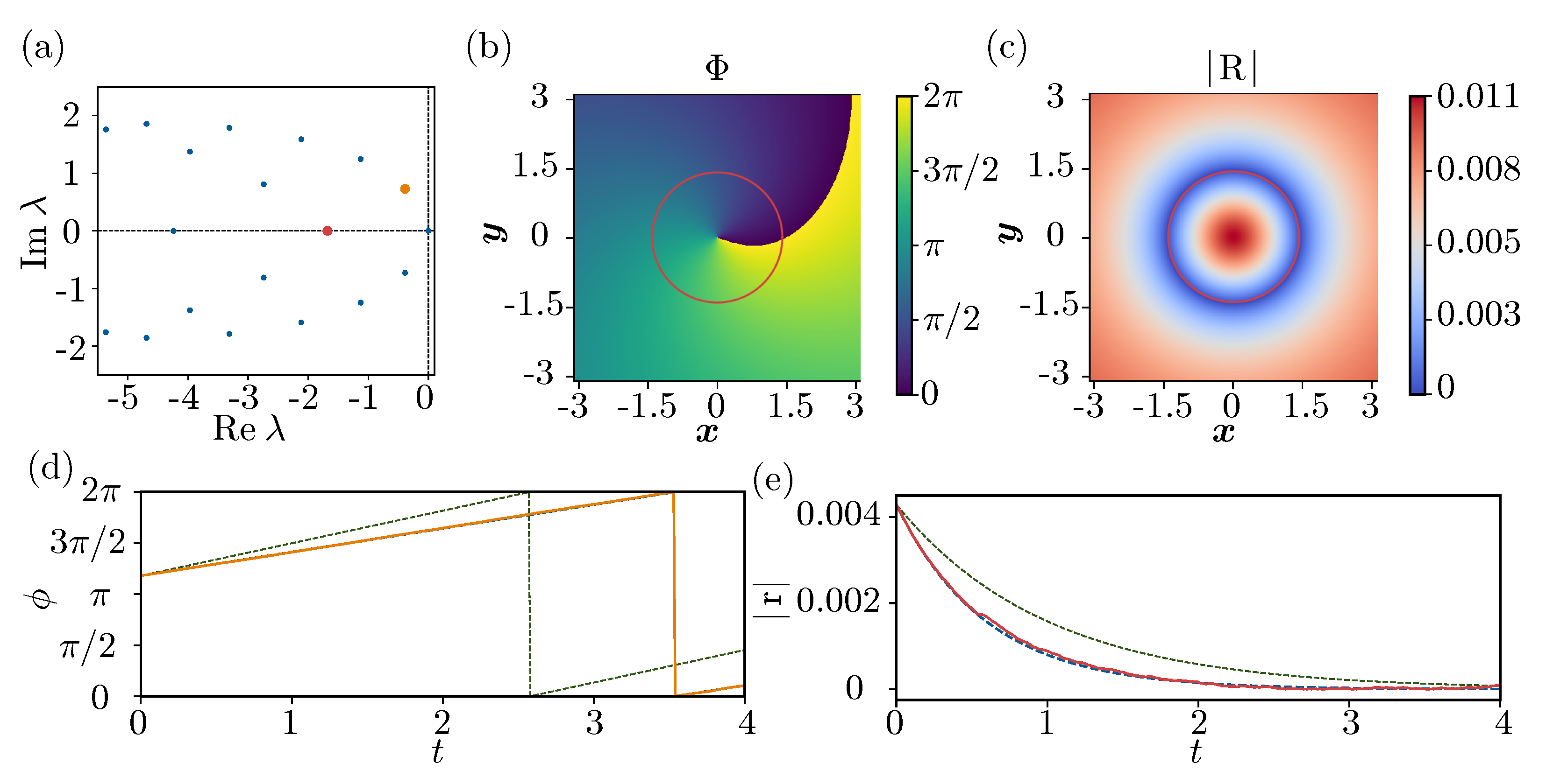
5.2. Example 1: Noisy Stuart–Landau Model

As the first example, we consider the Stuart–Landau model (the normal form of the supercritical Hopf bifurcation [2,42]) under the effect of noise, described by

$$\begin{array}{cc}\hfill dx& =\{ax-by-(cx-dy)(x^2+y^2)\}dt+\sqrt{D_x}d{W}_x,\hfill \\ \hfill dy& =\{bx+ay-(dx+cy)(x^2+y^2)\}dt+\sqrt{D_y}d{W}_y,\hfill \end{array}$$

(45)

where x and y are real variables, $a,b,c$, and d are real parameters, $W_x$ and $W_y$ are independent Wiener processes, and $D_x$ and $D_y$ represent the intensities of the noise acting on x and y, respectively. The noiseless system with $D_x=D_y=0$ has a stable limit cycle with a natural frequency $\omega =b-ad/c$ and the largest non-zero Floquet exponent ${\lambda }_1=-2a$ when $a>0$ and $c>0$. For this system, we can explicitly calculate the limit cycle and the phase and amplitude functions as [4]

$$\begin{array}{cc}\hfill & {(x_0\left(\varphi \right),y_0\left(\varphi \right))}^T=\sqrt{\frac{a}{c}}{(cos\varphi ,sin\varphi )}^T,\hfill \\ \hfill & {\Phi }_0(x,y)={tan}^{-1}\left(\frac{y}{x}\right)-\frac{d}{c}ln\sqrt{\frac{c}{a}(x^2+y^2)},\hfill \\ \hfill & R_0(x,y)=C_0\left(c-\frac{a}{x^2+y^2}\right).\hfill \end{array}$$

(46)

where $C_0$ is an arbitrary scalar constant. The basin $B_{\chi }$ of this limit cycle $\chi$ is the whole complex plane except the origin.

In the following numerical simulations, we set the parameter values as $(a,b,c,d,D_x,$$D_y)$$=(0.5,$$1.5$, $0.25$, $0.25$, 1, $1)$. The natural frequency and the largest non-zero Floquet exponent are $\omega =1$ and ${\lambda }_1=-1$, respectively. It is noted that the fundamental frequency ${\omega }_1=Im{\Lambda }_1$ and decay rate ${\Lambda }_2$ under the effect of noise are generally different from these deterministic values. We used $D=3.6$ and $N=151$ for the numerical analysis.

Figure 1a shows the eigenvalues of the Koopman operator $L_{\mathit{X}}^{+}$ near the imaginary axis obtained numerically, where the eigenvalues ${\Lambda }_1={\mu }_1+i{\omega }_1$ and ${\Lambda }_2$ are shown by orange and red dots, respectively. The rightmost branch of the eigenvalues is approximately given by a parabola ${\widehat{\lambda }}_n=i{\omega }_{1}n-{\mu }_1{n}^2(n=0,\pm 1,\pm 2,\dots )$ passing through ${\Lambda }_1$ [35].

Figure 1b,c show the phase function $\Phi (x,y)$ and amplitude function $\left|R(x,y)\right|$ associated with ${\Lambda }_1={\mu }_1+i{\omega }_1$ and ${\Lambda }_2$, respectively. We can observe that a circular region representing the local minima of the amplitude exists along the limit-cycle solution in the deterministic case and the phase increases from 0 to $2\pi$ along this circle. In contrast to the deterministic case, Equation (46), the amplitude does not diverge at the unstable fixed point at the origin $(x,y)=(0,0)$, because the system state can escape from this point in a finite time due to the effect of noise.

To confirm that these functions yield appropriate values of the phase and amplitude on average, we obtained 10,000 trajectories by direct numerical simulations of the Equation (45) from the initial point $(x_0,y_0)=(-1.5,-1.5)$ and calculated the averaged phase $\varphi =\mathrm{Arg}\left[\overline{Q_1}(x,y)\right]$ and amplitude $\left|r\right|=\left[|\overline{Q_2}(x,y)|\right]$, where $\left[·\right]$ represents a sample average over all obtained trajectories. Figure 1d,e show that these values are in good agreement with the analytical solutions $\varphi ={\omega }_{1}t+{\varphi }_0$ and $\left|r\right|=|r_0|exp\left({\Lambda }_{2}t\right)$, where the fundamental frequency ${\omega }_1=0.728$ and the decay rate ${\Lambda }_2=-1.680$ are numerically evaluated from the eigenvalues plotted in Figure 1a. For comparison, we also show the analytical solutions for the deterministic case without noise ($D_x=D_y=0$), namely, $\varphi =\omega t+{\varphi }_0=t+{\varphi }_0$ and $\left|r\right|=|r_0|exp\left({\lambda }_{1}t\right)=\left|r_0\right|exp(-t)$. The averaged phase increases more slowly and the averaged amplitude decays more quickly than those in the deterministic case due to the effect of noise.

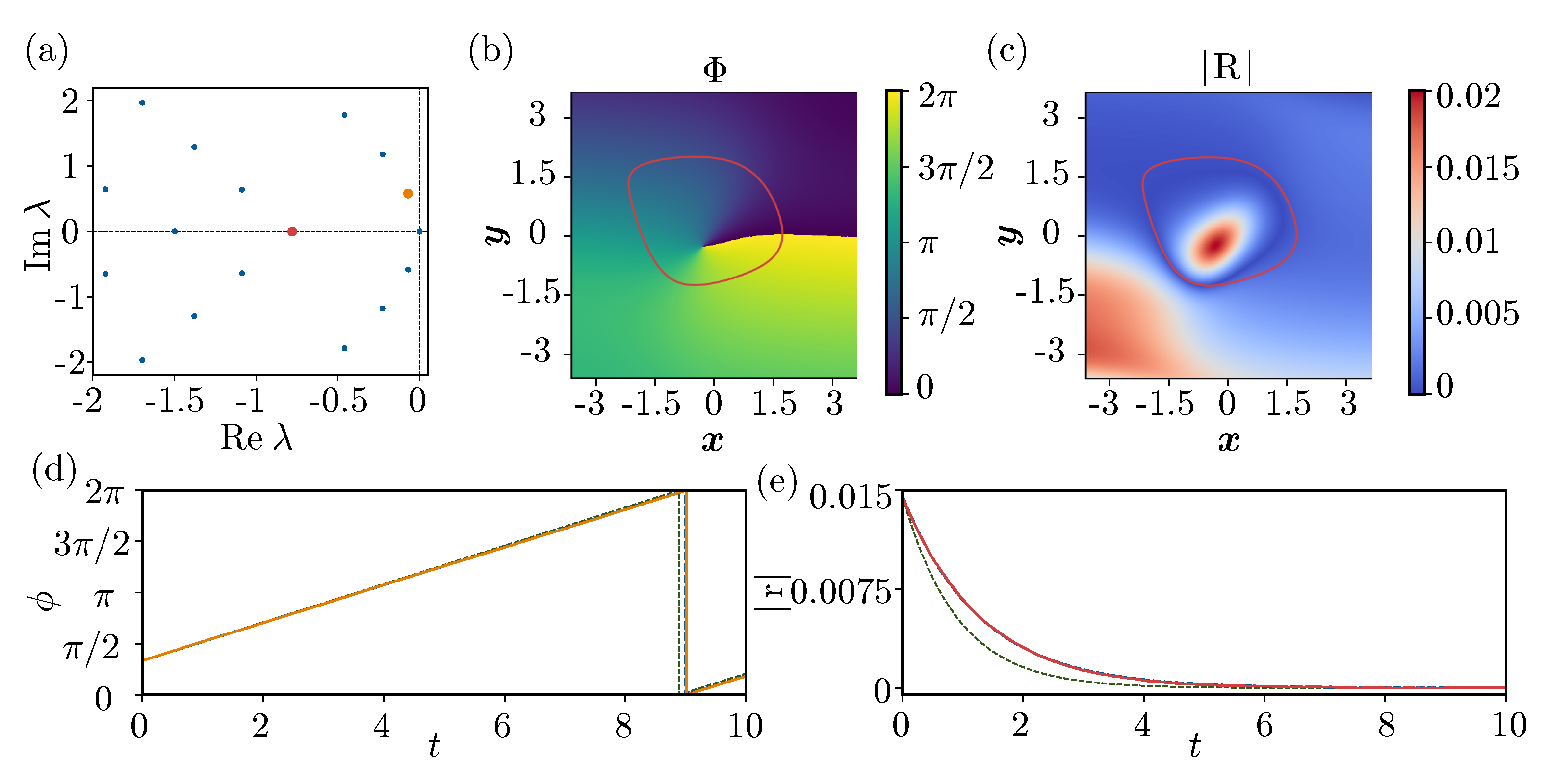
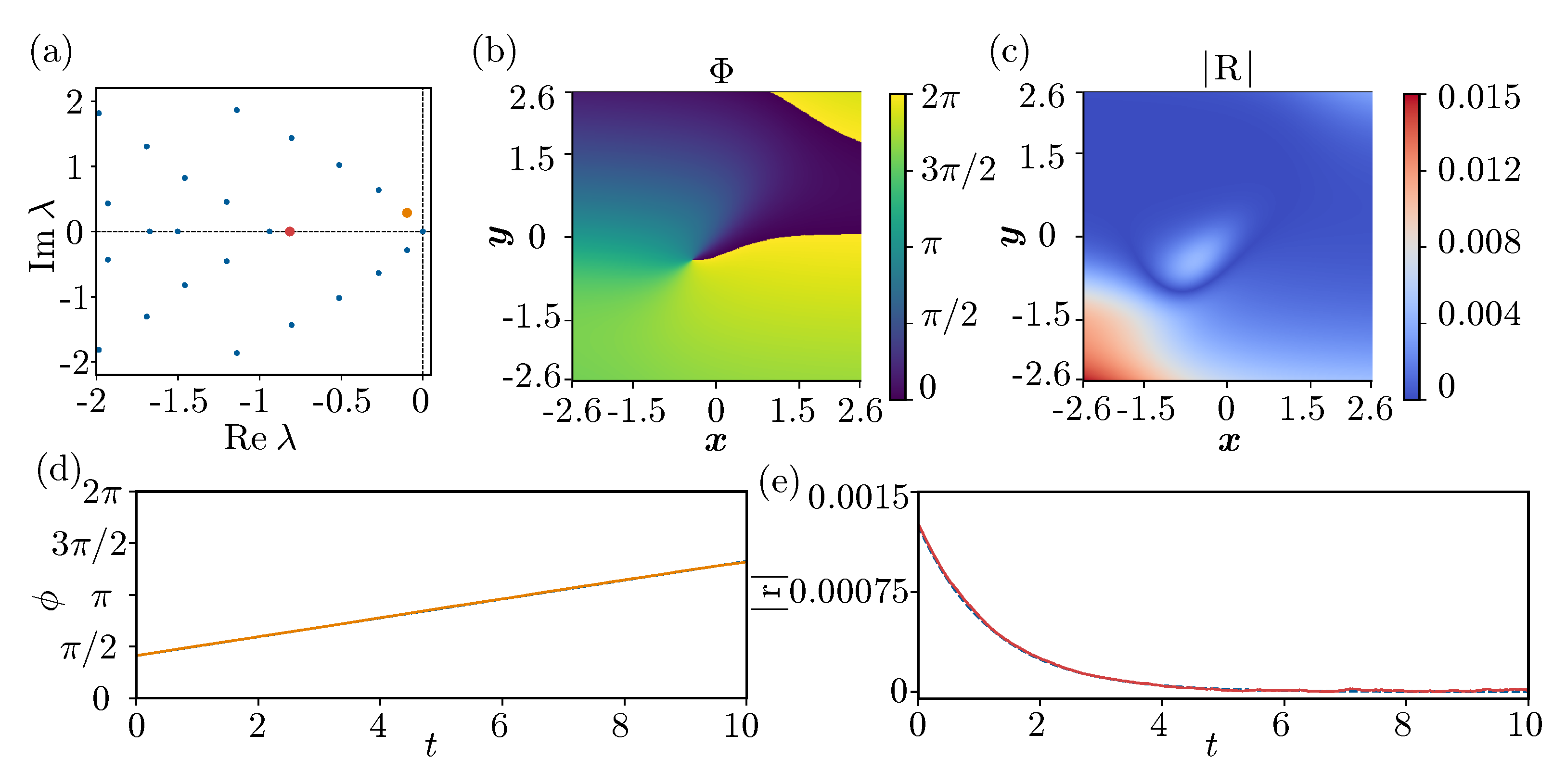
5.3. Example 2: Noisy FitzHugh–Nagumo Model

Next, we consider the FitzHugh–Nagumo model [40,41] subjected to noise, described by

$$\begin{array}{cc}\hfill dx& =(x-a_1{x}^3-y)dt+\sqrt{D_x}d{W}_x,\hfill \\ \hfill dy& ={\eta }_1(x+b_1)dt+\sqrt{D_y}d{W}_y,\hfill \end{array}$$

(47)

where x and y are real variables, $a_1$, $b_1$, and ${\eta }_1$ are real parameters, $W_x$ and $W_y$ are independent Wiener processes, and $D_x$ and $D_y$ represent the intensities of the noise, respectively.

First, we consider parameter set (A): $(a_1,b_1,$${\eta }_1,D_x,D_y)$$=(1/3,0.5,0.5,0.2,0.2)$, at which the deterministic vector field possesses a stable limit-cycle solution with the natural frequency $\omega =0.588$ and the largest non-zero Floquet exponent ${\lambda }_1=-1.11$. We used $D=4.2$ and $N=151$ for the numerical analysis.

Figure 2a shows the eigenvalues of the Koopman operator $L_{\mathit{X}}^{+}$ near the imaginary axis obtained numerically, where ${\Lambda }_1={\mu }_1+i{\omega }_1$ and ${\Lambda }_2$ are shown by orange and red dots, respectively. The rightmost branch of the eigenvalues is approximately a parabola ${\widehat{\lambda }}_n=i{\omega }_{1}n-{\mu }_1{n}^2(n=0,\pm 1,\pm 2,\dots )$ passing through ${\Lambda }_1$, which is qualitatively similar to the one for the noisy Stuart–Landau model in Figure 1a. Figure 2b,c show the phase $\Phi (x,y)$ and amplitude $\left|R(x,y)\right|$ associated with ${\Lambda }_1={\mu }_1+i{\omega }_1$ and ${\Lambda }_2$. As in the case of the noisy Stuart–Landau model, a circular region corresponding to the local minima of the amplitude function exists around the deterministic limit-cycle solution and the phase increases along this region. The amplitude does not diverge at the unstable fixed point due to the effect of noise.

We calculated the time evolution of $\Phi (x,y)$ and $\left|R(x,y)\right|$ by direct numerical simulations of Equation (47) from the initial point $(x_0,y_0)=(0.1,0.1)$ and averaged the results over 10,000 trajectories. Figure 2d,e show the averaged phase $\varphi =\mathrm{Arg}\left[\overline{Q_1}(x,y)\right]$ and amplitude $\left|r\right|=\left[|\overline{Q_2}(x,y)|\right]$. They are in good agreement with the analytical solutions $\varphi ={\omega }_{1}t+{\varphi }_0$ and $\left|r\right|=|r_0|exp\left({\Lambda }_{2}t\right)$, where the fundamental frequency ${\omega }_1=0.582$ and the decay rate ${\Lambda }_2=-0.778$ are numerically evaluated from the eigenvalues plotted in Figure 2a. For comparison, we also show the analytical solution for the deterministic case without noise ($D_x=D_y=0$), namely, $\varphi =\omega t+{\varphi }_0=0.588t+{\varphi }_0$ and $\left|r\right|=|r_0|exp\left({\lambda }_{1}t\right)=\left|r_0\right|exp(-1.11t)$. The phase evolves more slowly and also the amplitude decays more slowly than those in the deterministic case due to the effect of noise.

Next, we consider parameter set (B): $(a_1,b_1,$${\eta }_1,D_x,D_y)=(1/3,1.05,0.25,0.1,0.1)$. In this case, the deterministic vector field does not have a stable limit-cycle, but the system is close to a supercritical Hopf bifurcation of a limit cycle. Thus, relatively regular noise-induced oscillations occur even though the system does not have a deterministic limit cycle, a phenomenon known as the coherence resonance [54,55,56]. We used $D=3.9$ and $N=151$ for the numerical analysis.

Figure 3a shows the eigenvalues of the Koopman operator $L_{\mathit{X}}^{+}$ near the imaginary axis obtained numerically, where ${\Lambda }_1={\mu }_1+i{\omega }_1$ and ${\Lambda }_2$ are shown by orange and red dots, respectively. Figure 3b,c show the phase $\Phi (x,y)$ and amplitude $\left|R(x,y)\right|$ associated with ${\Lambda }_1={\mu }_1+i{\omega }_1$ and ${\Lambda }_2$, respectively. Interestingly, although the deterministic system does not have a limit-cycle solution, we can still observe in Figure 3b,c a circular region representing the local minima of the amplitude function. This region corresponds to the noise-induced oscillations and the phase increases along this circular region.

Figure 3d,e show the time evolution of the average values of the phase and amplitude, which are averaged over 10,000 trajectories by direct numerical simulations of the Equation (47) from the initial point $(x_0,y_0)=(0.1,0.1)$. The averaged phase $\varphi =\mathrm{Arg}\left[\overline{Q_1}(x,y)\right]$ and amplitude $r=\left[|\overline{Q_2}(x,y)|\right]$ show good agreement with the analytical solutions $\varphi ={\omega }_{1}t+{\varphi }_0$ and $\left|r\right|=|r_0|exp\left({\Lambda }_{2}t\right)$, where the fundamental frequency ${\omega }_1=0.287$ and the decay rate ${\Lambda }_2=-0.815$ are numerically evaluated from the eigenvalues in Figure 3a.

Thus, we can introduce the phase and amplitude functions also in this case without a deterministic limit cycle by using the present definition using the Koopman eigenfunctions.

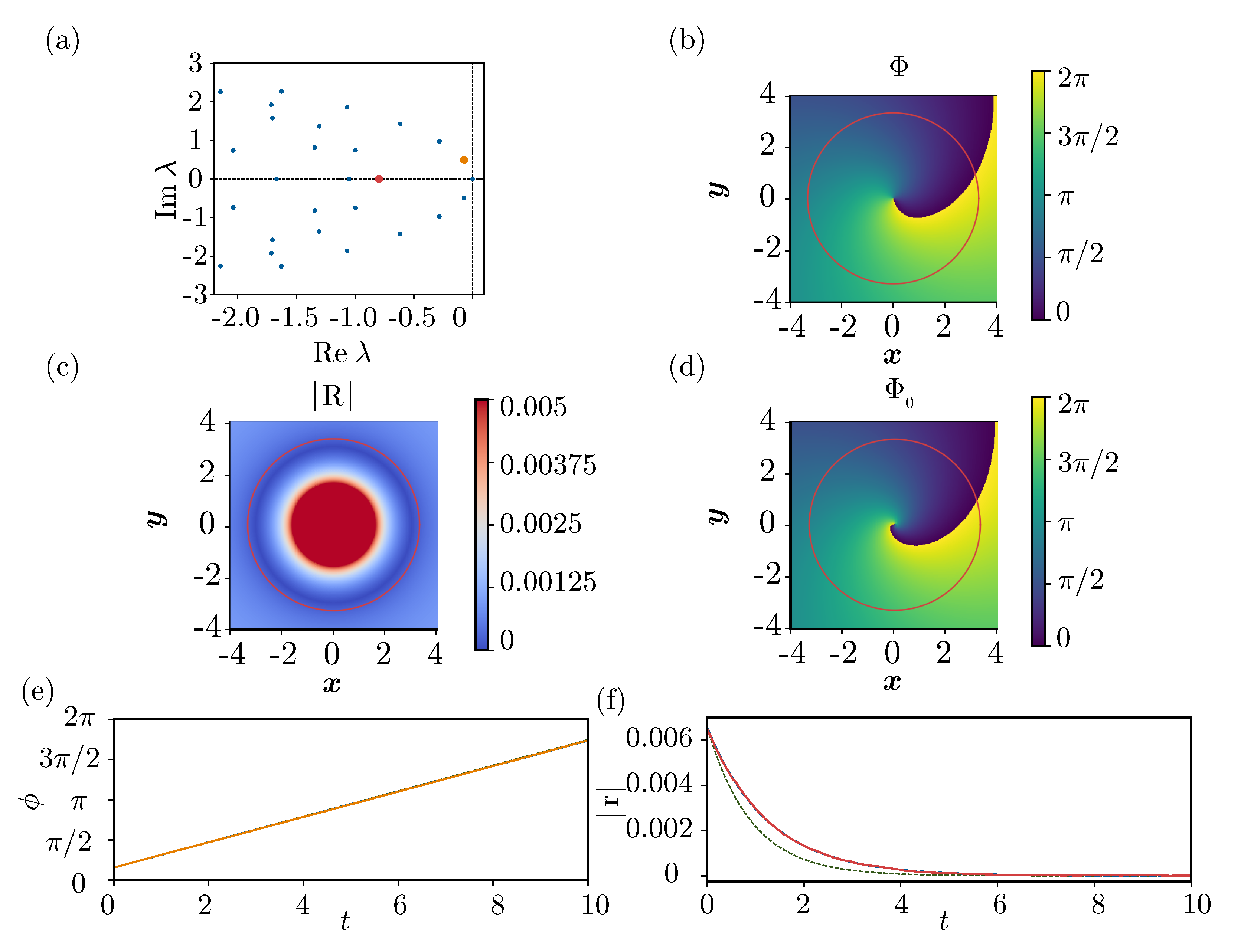
5.4. Example 3: Semiclassical Stuart–Landau Model

Finally, we apply the proposed definition of the stochastic phase and amplitude functions to a quantum limit-cycle oscillator in the semiclassical regime. As an example, we use the quantum Stuart–Landau model [57,58] (also known as the quantum van der Pol model [59]) with a Kerr effect [33,60] in quantum optics.

Employing the phase space approach [61,62], the system state can be represented by a Wigner function $W(x,y)$ (see References [33,60] for details). In the semiclassical regime, the quantum noise is sufficiently weak and $W(x,y)$ approximately obeys a quantum FPE, which has the same form as the ordinary FPE for classical systems. Thus, we can derive the corresponding Ito SDE from the quantum FPE as

$$\begin{array}{cc}\hfill d\left(\begin{array}{c}x\\ y\end{array}\right)& =\left(\begin{array}{c}\frac{{\gamma }_1+2{\gamma }_2}{2}x-({\omega }_0+2K)p-({\gamma }_{2}x-2Kp)(x^2+p^2)\\ ({\omega }_0+2K)x+\frac{{\gamma }_1+2{\gamma }_2}{2}p-(2Kx+{\gamma }_{2}p)(x^2+p^2)\end{array}\right)dt+\sqrt{\frac{\beta (x,y)}{2}}\left(\begin{array}{c}d{W}_x\\ d{W}_y\end{array}\right),\hfill \end{array}$$

(48)

where $\beta (x,y)=\frac{{\gamma }_1}{2}+2{\gamma }_2\left(x^2+y^2-\frac{1}{2}\right)$, ${\omega }_0$ is a frequency parameter of the oscillator, K represents the Kerr parameter, and ${\gamma }_1$ and ${\gamma }_2$ are the decay rates for the negative damping and nonlinear damping, respectively, and $W_x$ and $W_y$ are independent Wiener processes. The semiclassical approximation is valid when ${\gamma }_2$ and K are sufficiently small [33,60].

The deterministic part of Equation (48) is equivalent to the Stuart–Landau model used in Example 1 and only the coefficient of the noise term differs. Therefore, the deterministic limit cycle and the phase and amplitude functions can be obtained from the results for Equation (46), where the parameters are given by $a=\frac{{\gamma }_1+2{\gamma }_2}{2}$, $b={\omega }_0+2K,c={\gamma }_2,d=2K$. We set the parameter values as $({\gamma }_1,{\gamma }_2,{\omega }_0,K)=(1,0.05,1,0.025)$. With these values, the deterministic vector field of Equation (48) possesses a stable limit-cycle solution with the natural frequency $\omega ={\omega }_0-K{\gamma }_1/{\gamma }_2=0.5$ and the largest non-zero Floquet exponent ${\lambda }_1={\gamma }_1+2{\gamma }_2=-1.1$. We used $D=6.7$ and $N=151$ for the numerical analysis.

Figure 4a shows the eigenvalues of the Koopman operator $L_{\mathit{X}}^{+}$, where ${\Lambda }_1={\mu }_1+i{\omega }_1$ and ${\Lambda }_2$ are indicated by orange and red dots, respectively. Figure 4b,c show the phase function $\Phi (x,y)$ and amplitude function $R(x,y)$ associated with ${\Lambda }_1={\mu }_1+i{\omega }_1$ and ${\Lambda }_2$. For comparison, we also show in Figure 4d the deterministic phase function ${\Phi }_0(x,y)$ in Equation (46). The stochastic phase function $\Phi (x,y)$ in Figure 4b is slightly different from the deterministic phase function ${\Phi }_0(x,y)$ in Figure 4d, in particular near the origin, because the stochastic phase function includes the effect of weak quantum noise. Figure 4c shows that the amplitude function takes the minima around the deterministic limit cycle. We note that the amplitude function does not diverge at the origin in contrast to the deterministic case. Here, we used a color map with the maximum value of $0.005$ to enhance the local minima of the amplitude function, and the region near the origin where the amplitude is larger than $0.005$ is shown in the same color (the true maximum amplitude is $0.0876$ at the origin).

Figure 4e,f show the time evolution of the values of the phase and amplitude averaged over 10,000 trajectories obtained by direct numerical simulations of the semiclassical Equation (45) from the initial point $(x_0,y_0)=(2.5,0)$. They show good agreement with the analytical solutions $\varphi ={\omega }_{1}t+{\varphi }_0$ and $\left|r\right|=|r_0|exp\left({\Lambda }_{2}t\right)$, where the values of the fundamental frequency ${\omega }_1=0.496$ and the decay rate ${\Lambda }_2=-0.798$ are numerically evaluated from the eigenvalues shown in Figure 4a.

Thus, the present definition of the phase and amplitude functions is also applicable to a quantum Stuart–Landau model in the semiclassical regime and yields reasonable values.

6. Discussion

We proposed a definition of the asymptotic phase and amplitude functions for stochastic oscillatory systems by generalizing the definition for deterministic limit-cycle oscillators on the basis of the Koopman operator theory, motivated by the definition of the stochastic asymptotic phase introduced by Thomas and Lindner [35].

The proposed asymptotic phase and amplitude for strongly stochastic oscillatory systems may be used for systematic and quantitative analysis of synchronization phenomena in stochastic oscillators. We may also be able to develop a phase-amplitude reduction theory for strongly stochastic oscillators by using the phase and amplitude functions, which allows us to reduce the system dynamics subjected to weak external inputs to a simple two-dimensional set of equations. Such theories will facilitate detailed analysis, control, and optimization of noise-induced oscillatory phenomena, including the coherence-resonance and self-induced-stochastic-resonance oscillations [63,64].

It will also be interesting to introduce amplitude functions for strongly quantum oscillatory systems on the basis of the Koopman operator theory [38]. We have recently defined the quantum asymptotic phase of strongly quantum oscillators by using the eigenoperator of the adjoint Liouville superoperator and found that it can largely differ from the asymptotic phase in the classical limit [38]. The amplitude function, which can be defined similarly, may also be very different from the classical counterpart and characterize the quantum signatures of synchronization observed in the strong quantum regime.

7. Conclusions

We proposed a definition of the asymptotic phase and amplitude functions for stochastic oscillatory systems. The proposed phase and amplitude functions are introduced in terms of the backward Fokker–Planck operator, which can be interpreted as the Koopman operator for the stochastic system. The validity of the phase and amplitude functions was numerically demonstrated for noisy Stuart–Landau and FitzHugh–Nagumo models and also for a quantum Stuart–Landau model in the semiclassical regime.

Note added—During the preparation of this article, we noticed a new, closely related study by Pérez-Cervera, Lindner, and Thomas [65], which introduced the isostables (level sets of the asymptotic amplitude function) for stochastic oscillators on the basis of the backward Kolmogorov equation and analyzed the examples of a spiral sink, a noisy Stuart–Landau oscillator, and a noisy heteroclinic oscillator. Our present results differ from Reference [65] in that we explicitly discussed the relationship with the Koopman operator theory and analyzed a noisy excitable system and quantum limit-cycle oscillator in the semiclassical regime, in addition to noisy limit-cycle oscillators. We thus believe our results provide different insights and are complementary to Reference [65].

References

1. Winfree, A.T. The Geometry of Biological Time; Springer: Berlin/Heidelberg, Germany, 2001. [Google Scholar]
2. Kuramoto, Y. Chemical Oscillations, Waves, and Turbulence; Springer: Berlin/Heidelberg, Germany, 1984. [Google Scholar]
3. Pikovsky, A.; Rosenblum, M.; Kurths, J. Synchronization: A Universal Concept in Nonlinear Sciences; Cambridge University Press: Cambridge, UK, 2001. [Google Scholar]
4. Nakao, H. Phase reduction approach to synchronisation of nonlinear oscillators. Contemp. Phys. 2016, 57, 188–214. [Google Scholar] [CrossRef] [Green Version]
5. Ermentrout, G.B.; Terman, D.H. Mathematical Foundations of Neuroscience; Springer: Berlin/Heidelberg, Germany, 2010. [Google Scholar]
6. Strogatz, S. Nonlinear Dynamics and Chaos; Westview Press: Boulder, CO, USA, 1994. [Google Scholar]
7. Hoppensteadt, F.C.; Izhikevich, E.M. Weakly Connected Neural Networks; Springer: Berlin/Heidelberg, Germany, 1997; Volume 126. [Google Scholar]
8. Winfree, A.T. Biological rhythms and the behavior of populations of coupled oscillators. J. Theor. Biol. 1967, 16, 15–42. [Google Scholar] [CrossRef]
9. Guckenheimer, J. Isochrons and phaseless sets. J. Math. Biol. 1975, 1, 259–273. [Google Scholar] [CrossRef] [PubMed]
10. Mauroy, A.; Mezić, I.; Moehlis, J. Isostables, isochrons, and Koopman spectrum for the action–angle representation of stable fixed point dynamics. Phys. D Nonlinear Phenom. 2013, 261, 19–30. [Google Scholar] [CrossRef] [Green Version]
11. Mauroy, A.; Susuki, Y.; Mezić, I. Introduction to the Koopman operator in systems and control theory. In The Koopman Operator in Systems and Control; Springer: Berlin/Heidelberg, Germany, 2020; pp. 3–33. [Google Scholar]
12. Shirasaka, S.; Kurebayashi, W.; Nakao, H. Phase-amplitude reduction of transient dynamics far from attractors for limit-cycling systems. Chaos 2017, 27, 023119. [Google Scholar] [CrossRef] [PubMed] [Green Version]
13. Kuramoto, Y.; Nakao, H. On the concept of dynamical reduction: The case of coupled oscillators. Philos. Trans. R. Soc. A 2019, 377, 20190041. [Google Scholar] [CrossRef] [Green Version]
14. Shirasaka, S.; Kurebayashi, W.; Nakao, H. Phase-Amplitude Reduction of Limit Cycling Systems. In The Koopman Operator in Systems and Control; Springer: Berlin/Heidelberg, Germany, 2020; pp. 383–417. [Google Scholar]
15. Hale, J. Ordinary Differential Equations; Dover Publications: Mineola, NY, USA, 2009. [Google Scholar]
16. Revzen, S.; Guckenheimer, J.M. Finding the dimension of slow dynamics in a rhythmic system. J. R. Soc. Interface 2012, 9, 957–971. [Google Scholar] [CrossRef] [Green Version]
17. Kvalheim, M.D.; Revzen, S. Existence and uniqueness of global Koopman eigenfunctions for stable fixed points and periodic orbits. Phys. Nonlinear Phenom. 2021, 425, 132959. [Google Scholar] [CrossRef]
18. Mauroy, A.; Mezić, I. Global computation of phase-amplitude reduction for limit-cycle dynamics. Chaos Interdiscip. J. Nonlinear Sci. 2018, 28, 073108. [Google Scholar] [CrossRef] [Green Version]
19. Wilson, D.; Moehlis, J. Isostable reduction of periodic orbits. Phys. Rev. E 2016, 94, 052213. [Google Scholar] [CrossRef] [Green Version]
20. Monga, B.; Wilson, D.; Matchen, T.; Moehlis, J. Phase reduction and phase-based optimal control for biological systems: A tutorial. Biol. Cybern. 2019, 113, 11–46. [Google Scholar] [CrossRef]
21. Monga, B.; Moehlis, J. Optimal phase control of biological oscillators using augmented phase reduction. Biol. Cybern. 2019, 113, 161–178. [Google Scholar] [CrossRef]
22. Zlotnik, A.; Chen, Y.; Kiss, I.Z.; Tanaka, H.A.; Li, J.S. Optimal waveform for fast entrainment of weakly forced nonlinear oscillators. Phys. Rev. Lett. 2013, 111, 024102. [Google Scholar] [CrossRef] [PubMed]
23. Kato, Y.; Zlotnik, A.; Li, J.S.; Nakao, H. Optimization of periodic input waveforms for global entrainment of weakly forced limit-cycle oscillators. arXiv 2021, arXiv:2103.02880. [Google Scholar]
24. Takata, S.; Kato, Y.; Nakao, H. Fast optimal entrainment of limit-cycle oscillators by strong periodic inputs via phase-amplitude reduction and Floquet theory. arXiv 2021, arXiv:2104.09944. [Google Scholar]
25. Kotani, K.; Ogawa, Y.; Shirasaka, S.; Akao, A.; Jimbo, Y.; Nakao, H. Nonlinear phase-amplitude reduction of delay-induced oscillations. Phys. Rev. Res. 2020, 2, 033106. [Google Scholar] [CrossRef]
26. Nakao, H. Phase and amplitude description of complex oscillatory patterns in reaction-diffusion systems. In Physics of Biological Oscillators; Springer: Berlin/Heidelberg, Germany, 2021; pp. 11–27. [Google Scholar]
27. Teramae, J.; Nakao, H.; Ermentrout, G.B. Stochastic phase reduction for a general class of noisy limit cycle oscillators. Phys. Rev. Lett. 2009, 102, 194102. [Google Scholar] [CrossRef] [Green Version]
28. Goldobin, D.S.; Teramae, J.n.; Nakao, H.; Ermentrout, G.B. Dynamics of limit-cycle oscillators subject to general noise. Phys. Rev. Lett. 2010, 105, 154101. [Google Scholar] [CrossRef] [Green Version]
29. Nakao, H.; Teramae, J.N.; Goldobin, D.S.; Kuramoto, Y. Effective long-time phase dynamics of limit-cycle oscillators driven by weak colored noise. Chaos Interdiscip. J. Nonlinear Sci. 2010, 20, 033126. [Google Scholar] [CrossRef] [Green Version]
30. Bonnin, M. Phase oscillator model for noisy oscillators. Eur. Phys. J. Spec. Top. 2017, 226, 3227–3237. [Google Scholar] [CrossRef]
31. Bonnin, M. Amplitude and phase dynamics of noisy oscillators. Int. J. Circuit Theory Appl. 2017, 45, 636–659. [Google Scholar] [CrossRef] [Green Version]
32. Aminzare, Z.; Holmes, P.; Srivastava, V. On Phase Reduction and Time Period of Noisy Oscillators. In Proceedings of the 2019 IEEE 58th Conference on Decision and Control (CDC), Nice, France, 11–13 December 2019; pp. 4717–4722. [Google Scholar]
33. Kato, Y.; Yamamoto, N.; Nakao, H. Semiclassical phase reduction theory for quantum synchronization. Phys. Rev. Res. 2019, 1, 033012. [Google Scholar] [CrossRef] [Green Version]
34. Schwabedal, J.T.; Pikovsky, A. Phase description of stochastic oscillations. Phys. Rev. Lett. 2013, 110, 204102. [Google Scholar] [CrossRef] [Green Version]
35. Thomas, P.J.; Lindner, B. Asymptotic phase for stochastic oscillators. Phys. Rev. Lett. 2014, 113, 254101. [Google Scholar] [CrossRef] [PubMed] [Green Version]
36. Cao, A.; Lindner, B.; Thomas, P.J. A Partial Differential Equation for the Mean–Return-Time Phase of Planar Stochastic Oscillators. SIAM J. Appl. Math. 2020, 80, 422–447. [Google Scholar] [CrossRef] [Green Version]
37. Kato, Y.; Nakao, H. Semiclassical optimization of entrainment stability and phase coherence in weakly forced quantum limit-cycle oscillators. Phys. Rev. E 2020, 101, 012210. [Google Scholar] [CrossRef] [PubMed] [Green Version]
38. Kato, Y.; Nakao, H. Quantum asymptotic phase reveals signatures of quantum synchronization. arXiv 2020, arXiv:2006.00760. [Google Scholar]
39. Engel, M.; Kuehn, C. A Random Dynamical Systems Perspective on Isochronicity for Stochastic Oscillations. Commun. Math. Phys. 2021, 386, 1–39. [Google Scholar] [CrossRef]
40. FitzHugh, R. Impulses and physiological states in theoretical models of nerve membrane. Biophys. J. 1961, 1, 445. [Google Scholar] [CrossRef] [Green Version]
41. Nagumo, J.; Arimoto, S.; Yoshizawa, S. An active pulse transmission line simulating nerve axon. Proc. IRE 1962, 50, 2061–2070. [Google Scholar] [CrossRef]
42. Guckenheimer, J.; Holmes, P. Nonlinear Oscillations, Dynamical Systems, and Bifurcations of Vector Fields; Springer: Berlin/Heidelberg, Germany, 1982. [Google Scholar]
43. Mauroy, A.; Mezić, I. On the use of Fourier averages to compute the global isochrons of (quasi) periodic dynamics. Chaos Interdiscip. J. Nonlinear Sci. 2012, 22, 033112. [Google Scholar] [CrossRef] [Green Version]
44. Arnold, L. Stochastic Differential Equations; John Wiley & Sons: Hoboken, NJ, USA, 1974. [Google Scholar]
45. Gardiner, C. Stochastic Methods; Springer: Berlin/Heidelberg, Germany, 2009. [Google Scholar]
46. Pavliotis, G.A. Stochastic Processes and Applications: Diffusion Processes, the Fokker-Planck and Langevin Equations; Springer: Berlin/Heidelberg, Germany, 2014; Volume 60. [Google Scholar]
47. Lasota, A.; Mackey, M.C. Probabilistic Properties of Deterministic Systems; Cambridge University Press: Cambridge, UK, 2008. [Google Scholar]
48. Lasota, A.; Mackey, M.C. Chaos, Fractals, and Noise: Stochastic Aspects of Dynamics; Springer Science & Business Media: Berlin/Heidelberg, Germany, 2013. [Google Scholar]
49. Risken, H. Fokker-planck equation. In The Fokker-Planck Equation; Springer: Berlin/Heidelberg, Germany, 1996; pp. 63–95. [Google Scholar]
50. Mezić, I. Spectral properties of dynamical systems, model reduction and decompositions. Nonlinear Dyn. 2005, 41, 309–325. [Google Scholar] [CrossRef]
51. Øksendal, B. Stochastic Differential Equations: An Introduction with Applications; Springer: Berlin/Heidelberg, Germany, 2000. [Google Scholar]
52. Fisher, N.I. Statistical Analysis of Circular Data; Cambridge University Press: Cambridge, UK, 1995. [Google Scholar]
53. Gaspard, P. Chaos, Scattering and Statistical Mechanics; Cambridge University Press: Cambridge, UK, 2005. [Google Scholar]
54. Gang, H.; Ditzinger, T.; Ning, C.Z.; Haken, H. Stochastic resonance without external periodic force. Phys. Rev. Lett. 1993, 71, 807. [Google Scholar] [CrossRef]
55. Pikovsky, A.S.; Kurths, J. Coherence resonance in a noise-driven excitable system. Phys. Rev. Lett. 1997, 78, 775. [Google Scholar] [CrossRef] [Green Version]
56. Lindner, B.; Schimansky-Geier, L. Coherence and stochastic resonance in a two-state system. Phys. Rev. E 2000, 61, 6103. [Google Scholar] [CrossRef] [Green Version]
57. Chia, A.; Kwek, L.; Noh, C. Relaxation oscillations and frequency entrainment in quantum mechanics. Phys. Rev. E 2020, 102, 042213. [Google Scholar] [CrossRef] [PubMed]
58. Arosh, L.B.; Cross, M.; Lifshitz, R. Quantum limit cycles and the Rayleigh and van der Pol oscillators. Phys. Rev. Res. 2021, 3, 013130. [Google Scholar] [CrossRef]
59. Lee, T.E.; Sadeghpour, H. Quantum synchronization of quantum van der Pol oscillators with trapped ions. Phys. Rev. Lett. 2013, 111, 234101. [Google Scholar] [CrossRef] [PubMed] [Green Version]
60. Lörch, N.; Amitai, E.; Nunnenkamp, A.; Bruder, C. Genuine quantum signatures in synchronization of anharmonic self-oscillators. Phys. Rev. Lett. 2016, 117, 073601. [Google Scholar] [CrossRef] [Green Version]
61. Gardiner, C.W. Quantum Noise; Springer: Berlin/Heidelberg, Germany, 1991. [Google Scholar]
62. Carmichael, H.J. Statistical Methods in Quantum Optics 1, 2; Springer: Berlin/Heidelberg, Germany, 2007. [Google Scholar]
63. Zhu, J. Phase sensitivity for coherence resonance oscillators. Nonlinear Dyn. 2020, 102, 2281–2293. [Google Scholar] [CrossRef]
64. Zhu, J.; Nakao, H. Stochastic periodic orbits in fast-slow systems with self-induced stochastic resonance. Phys. Rev. Res. 2021, 3, 033070. [Google Scholar] [CrossRef]
65. Pérez-Cervera, A.; Lindner, B.; Thomas, P.J. Isostables for stochastic oscillators. arXiv 2021, arXiv:2105.11048. [Google Scholar]
Figure 1. Phase and amplitude functions of a noisy Stuart–Landau model. (a) Eigenvalues of L X + near the imaginary axis. Orange and red dots represent Λ 1 and Λ 2 , respectively. (b) Phase function Φ ( x , y ) . The phase origin is chosen as ( x , p ) = ( 1.5 , 0 ) . (c) Amplitude function | R ( x , y ) | . (d) Evolution of averaged phase ϕ . (e) Evolution of averaged amplitude | r | . In (b,c), red-thin lines represent the deterministic limit-cycle solution. In (d,e), averaged results over 10,000 trajectories (orange and red thin lines) and analytical solutions (blue-dotted lines) for the stochastic case and results for the deterministic case (green-dotted lines) are shown.
Mathematics 09 02188 g001
Figure 2. Phase and amplitude functions of a noisy FitzHugh–Nagumo model with parameter set (A). The deterministic vector field possesses a limit-cycle solution. (a) Eigenvalues of L X + near the imaginary axis. Orange and red dots represent Λ 1 and Λ 2 , respectively. (b) Phase function Φ . (c) Amplitude function | R | . (d) Evolution of averaged phase ϕ . (d) Evolution of averaged amplitude | r | . In (b), ( x , p ) = ( 1.5 , 0 ) is chosen as the phase origin. In (b,c), red-thin lines represent the deterministic limit-cycle solution. In (d,e), averaged results over 10,000 trajectories (orange and red thin lines) and analytical solutions (blue-dotted lines) for the stochastic case and results for the deterministic case (green-dotted lines) are shown.
Mathematics 09 02188 g002
Figure 3. Phase and amplitude functions of a noisy FitzHugh–Nagumo model with parameter set (B). The deterministic vector field does not possess a limit cycle, but regular noise-induced oscillations occur. (a) Eigenvalues of L X + near the imaginary axis. Orange and red dots represent Λ 1 and Λ 2 , respectively. (b) Phase function Φ . The phase origin is chosen as ( x , p ) = ( 1.5 , 0 ) . (c) Amplitude function | R | . (d) Evolution of averaged phase ϕ . (e) Evolution of averaged amplitude | r | . In (d,e), averaged results over 10,000 trajectories (orange-thin or red-thin lines) and analytical solutions (blue-dotted lines) are shown.
Mathematics 09 02188 g003
Figure 4. Phase and amplitude functions of a quantum Stuart–Landau model with a quantum Kerr effect in the semiclassical regime. (a) Eigenvalues of L X + near the imaginary axis. Orange and red dots represent eigenvalues Λ 1 and Λ 2 , respectively. (b) Phase function Φ . (c) Amplitude function | R | . (d) Phase function Φ 0 of the deterministic system. (e) Evolution of averaged phase ϕ . (f) Evolution of averaged amplitude | r | . In (b,d), ( x , p ) = ( 2.5 , 0 ) is chosen as the phase origin. In (e,f), averaged results over 10,000 trajectories (orange and red thin lines) and analytical solutions for the semiclassical case (blue-dotted lines) and results for the deterministic case (green-dotted lines) are shown.
Mathematics 09 02188 g004
Publisher’s Note: MDPI stays neutral with regard to jurisdictional claims in published maps and institutional affiliations.