Article

A Convex Data-Driven Approach for Nonlinear Control Synthesis

1
Energy Storage Technology and Systems at Sandia National Laboratories, Albuquerque, NM 87185, USA
2
Department of Mechanical Enginerring, Clemson University, Clemson, SC 29634, USA
3
School of Aerospace Engineering, Georgia Institute of Technology, Atlanta, GA 30332, USA
*
Author to whom correspondence should be addressed.
Mathematics 2021, 9(19), 2445; https://doi.org/10.3390/math9192445
Submission received: 5 September 2021 / Revised: 22 September 2021 / Accepted: 22 September 2021 / Published: 1 October 2021
(This article belongs to the Special Issue Dynamical Systems and Operator Theory)

Abstract

:
We consider a class of nonlinear control synthesis problems where the underlying mathematical models are not explicitly known. We propose a data-driven approach to stabilize the systems when only sample trajectories of the dynamics are accessible. Our method is built on the density-function-based stability certificate that is the dual to the Lyapunov function for dynamic systems. Unlike Lyapunov-based methods, density functions lead to a convex formulation for a joint search of the control strategy and the stability certificate. This type of convex problem can be solved efficiently using the machinery of the sum of squares (SOS). For the data-driven part, we exploit the fact that the duality results in the stability theory can be understood through the lens of Perron–Frobenius and Koopman operators. This allows us to use data-driven methods to approximate these operators and combine them with the SOS techniques to establish a convex formulation of control synthesis. The efficacy of the proposed approach is demonstrated through several examples.

1. Introduction

The celebrated Lyapunov theory lays the foundation of stability analysis for general nonlinear dynamical systems. Lyapunov functions provide stability certificates for a nonlinear system. For a given system, searching for a proper Lyapunov function can often be formulated as a convex optimization problem, and thus is easy to address. For instance, for polynomial dynamics, this is achieved through the sum of squares (SOS). Regardless of its similarity to stability analysis, the problem of nonlinear controller synthesis is much more challenging. Other than a few special cases such as linear quadratic control problems, the joint search for Lyapunov stability certificate and control strategy can no longer be cast as convex optimization problems. This is exacerbated by the fact that in many applications, the underlying mathematical models are not available. Our objective in this paper is to establish a principled approach for nonlinear control synthesis when the mathematical models of the underlying dynamics are not explicitly given.
We provide a systematic approach for data-driven control synthesis for a class of control-affine nonlinear systems of the form
x ˙ = F ( x ) + G ( x ) u ,
where the state x R n and control inputs u R m , F represent the open-loop dynamics, and G ( x ) = [ G 1 ( x ) , , G m ( x ) ] constitutes the feedback control loop corresponding to control inputs u = [ u 1 , , u m ] . The objective is to design a state feedback controller u = u ( x ) such that the closed-loop system is asymptotically stable. To achieve this objective, we use density function-based dual stability formulation introduced by Rantzer for almost everywhere stability analysis and synthesis for nonlinear control systems [1]. Unlike the Lyapunov function-based approach for control design, the co-design problem of simultaneously finding the density function and almost everywhere stabilizing controller can be written as a convex optimization problem. We exploit this convexity property for data-driven control synthesis. In [2,3], it was shown that the duality between density and Lyapunov function in the stability theory could be understood using the linear operator theoretic framework. In particular, the duality between Koopman and Perron–Frobenius operators is at the heart of the duality in the stability theory. This linear operator theoretic framework is also exploited for the data-driven control design [4,5].
The recent advances in data-driven approximation of the Koopman operator are used to discover a data-driven approach for the nonlinear control synthesis. In Koopman theory, a nonlinear system is lifted to an, albeit infinite-dimensional, linear system. This lifting can be approximated using data generated from the underlying nonlinear dynamics by the well-known Extended Dynamic Mode Decomposition (EDMD) algorithm [6]. These tools have been successfully applied in many domains such as fluid dynamics [7] and power systems [8,9], to understand the principle components/modes of given nonlinear dynamics [10]. Recently, Koopman theory has been introduced to the control synthesis tasks, in the hopes that a controller designed in the lifted space could be easier than that in the original state space. It turns out to be a challenging problem, since the lifting argument in the presence of control is no longer valid. Regardless of the progress that has been made in this direction during the last few years [11,12,13,14], a principled data-driven framework for nonlinear control synthesis is not yet available.
We use the EDMD algorithm combined with the duality results for the data-driven approximation of the Perron–Frobenius (P-F) operator corresponding to the control system. This linear P-F operator for the control system is then used to formulate a convex optimization problem for control synthesis. This optimization is over polynomials and can be solved using the SOS solvers. The complexity of the resulting optimization problem depends on the polynomial basis used to approximate the linear operators. Since control often does not require high-fidelity models, we expect to construct a reliable controller using a relatively small number of basis functions. We envision that this method can be applied to low-dimensional and medium-dimensional dynamical systems (e.g., robotics, distributedpower-electronics control applications).
Recently, several methods have been developed for control synthesis [15,16]. One major difference is that [15,16] focus on polynomial dynamics, while our methods applies to more general systems. Another important difference is that we use a stronger notion of stability compared with [16]. Another line of research that is related to this work is optimal control synthesis based on generalized moment problems. One major difference between [17] and our method is that we use a rational parametrization for the control strategy.
The rest of the paper is organized as follows. In Section 2, we provide a review on density function methods, SOS, and Koopman theory; these are the components of our approach. A stronger notion of stability is discussed in Section 3. Problem formulation and the details of our method are presented in Section 4. This is followed by several numerical examples in Section 5, and a short concluding remark in Section 6.

2. Background

Our proposed method for control synthesis utilizes the density function method for controller design, SOS for polynomial optimization and Koopman theory for data-driven approximations. Necessary background information on these components is discussed in this section.

2.1. Density Function Approach for Control Synthesis

Consider a control-affine system (1) with a feedback control strategy u ( x ) . It is well known that the closed-loop system is asymptotically stable with respect to the origin x = 0 if a Lyapunov function V exists, such that
V x ( F ( x ) + G ( x ) u ( x ) ) < 0 , x 0 .
Thus, for the purpose of control synthesis, one seeks a pair ( V , u ) so that (2) holds. Note that this inequality is bilinear with respect to V , u and thus the problem is non-convex. This is a major obstacle preventing the Lyapunov theory from being widely used in control synthesis. In [1], a dual to Lyapunov’s stability theorem was established.
Theorem 1
([1]). Given the system x ˙ = F ( x ) , where F is continuously differentiable and F ( 0 ) = 0 , suppose there exists a nonnegative ρ that is continuously differentiable for x 0 such that ρ ( x ) F ( x ) / | x | is integrable on { x R n : | x | 1 } and
[ · ( ρ F ) ] ( x ) > 0 f o r   a l m o s t   a l l x .
Then, for almost all initial states x ( 0 ) , the trajectory x ( t ) tends to zero as t . Moreover, if the equilibrium x = 0 is stable, then the conclusion remains valid even if ρ takes negative values.
The density ρ serves as a stability certificate and can be viewed as a dual to the Lyapunov function [1]. Applying Theorem 1 to the closed-loop system, we arrive at
· ( ρ ( F + G u ) ) > 0 for   almost   all x .
The control synthesis problem becomes that of searching for a pair ( ρ , u ) of functions so that (4) holds. Even though (4) is again bilinear, it becomes linear in terms of ( ρ , ρ u ) . Thus, the density-function-based method for control synthesis is a convex problem.

2.2. Sum of Squares

SOS [18,19,20,21] is a powerful technique to solve polynomial optimization with positive polynomial constraints. Briefly, SOS polynomials are a set of polynomials which can be described as a non-negative linear combination of a square of polynomials, that is, a polynomial of the form p = i = 1 d i p i 2 , where p i are polynomials and d i are non-negative coefficients. Clearly, SOS is a sufficient condition for the non-negativity of a polynomial. Hence, SOS relaxation provides a lower bound on the minimization problems of polynomial optimizations. Using the SOS relaxation, a large class of polynomial optimization problems with positive constraints can be formulated as SOS optimization:
min d w d s . t . p s ( x ; d ) Σ [ x ] , p e ( x ; d ) = 0 ,
where Σ [ x ] denotes an SOS set, w consists of weighting coefficients, and p s ,   p e are polynomials with coefficients d . The problem in (5) can be converted into Semidefinite Programming (SDP) [19,22]. There are readily available SOS optimization packages, such as SOSTOOLS [23] and SOSOPT [24] that are designed to solve (5).

2.3. Linear Koopman and Perron–Frobenius Operators

For a dynamical system, x ˙ = F ( x ) , there are two different ways of linearly lifting the finite dimensional nonlinear dynamics from state space to some infinite dimension space of functions F . They are the Koopman operator and Perron–Frobenius operator. The solution of system (1) with zero control is denoted by s t ( x ) . The definitions of these operators, along with the corresponding infinitesimal generators, are as follows.
Definition 1
(Koopman Operator). K t : F F for dynamical system (1) is defined as
[ K t φ ] ( x ) = φ ( s t ( x ) ) , φ F , t 0 .
The infinitesimal generator for the Koopman operator is
lim t 0 K t φ φ t = F ( x ) · φ ( x ) = : K F φ .
Definition 2
(Perron–Frobenius Operator). P t : F F for dynamical system (1) is defined as
[ P t ψ ] ( x ) = ψ ( s t ( x ) ) s t ( x ) x , ψ F , t 0
where · stands for the determinant. The infinitesimal generator for the P-F operator is given by
lim t 0 P t ψ ψ t = · ( F ( x ) ψ ( x ) ) = : P F ψ .
These two operators are dual to each other, where the duality is expressed as
R n [ K t φ ] ( x ) ψ ( x ) d x = R n [ P t ψ ] ( x ) φ ( x ) d x .

3. Stabilization with Stronger Notion of Stability

In this section, we present a stronger notion of stability than that in Theorem 1. Consider the following dynamical system without control:
x ˙ = F ( x ) .
Assumption 1.
Assume that x = 0 is a locally stable equilibrium point for the system (9) with a local domain of attraction denoted by N . Let B δ be the neighborhood of the origin for any given fixed δ > 0 such that 0 B δ N . Denote X 1 : = R n B δ .
Definition 3
(Almost everywhere uniform stability). The equilibrium point x = 0 satisfying Assumption 1 is said to be almost everywhere uniform stable with respect to finite measure μ if for every ϵ > 0 there exists a time T ( ϵ ) such that
T ( ϵ ) μ ( A t ) d t < ϵ
where
A t : = { x R n : s t ( x ) A }
for any set A X 1 .
The following theorem from Theorem 13 [3] provides a sufficient condition for almost everywhere uniform stability.
Theorem 2.
The equilibrium point satisfying Assumption 1 is almost everywhere uniform stable with respect to measure μ with density h if a density function ρ C 1 ( R n { 0 } , R + ) exists that is integrable over X 1 and satisfies
· ( F ( x ) ρ ( x ) ) = h ( x ) .
Definition 4
(Almost everywhere geometric stability). The equilibrium point is said to be almost everywhere uniformly exponential stable if a positive constant β > 0 exists and for every ϵ > 0 , a time T ( ϵ ) exists, such that
T ( ϵ ) e β t μ ( A t ) < ϵ ,
where A t : = { x R n : s t ( x ) A } for any set A X 1 .
Next, we establish a sufficient condition that resembles (11) for geometric stability.
Theorem 3.
The equilibrium point x = 0 for system (9) satisfying Assumption 1 is almost everywhere stable with geometric decay with respect to measure μ with density h if a density function ρ ( x ) C 1 ( R n { 0 } , R + ) exists which is integrable on X 1 and satisfies
· ( F ρ ) = β ρ ( x ) + h
for some positive constant β > 0 .
Proof. 
Equation (13) can be rewritten as
i = 1 n F i ( x ) ρ x i + · ( F ( x ) β n x ) ρ ( x ) = h ( x ) .
Since (14) is a first-order PDE, we can use the method of characteristics to obtain a solution. The characteristic curves are given by the solution of the following ODE:
x ˙ ( t ) = F ( x ) .
Let F ˜ ( x ) = F ( x ) β n x , then Equation (14) can be rewritten as
d d t ρ ( s t ( x ) ) + ρ ( s t ( x ) ) · F ˜ = h ( s t ( x ) ) ,
which is a first-order ODE in the t variable.
The solution to (16) is obtained by multiplying (16) by the integrating factor exp { 0 t · F ˜ ( s τ ( x ) ) d τ } , which points to
d d t ( ρ ( s t ( x ) ) exp { 0 t · F ˜ ( s τ ( x ) ) d τ } ) = exp { 0 t · F ˜ ( s τ ( x ) ) d τ } h ( s t ( x ) ) .
It follows
exp { 0 t · F ˜ ( s τ ( x ) ) d τ } ρ ( s t ( x ) ) = ρ ( s 0 ( x ) ) + 0 t exp { 0 s · F ˜ ( x ( τ ) ) d τ } h ( s s ( x ) ) d s .
In view of | d ( s t ( x ) ) d x | = exp { 0 t · F ( s τ ( x ) ) d τ } and
exp { 0 t · F ˜ ( s τ ( x ) ) d τ } = exp { β t } exp { 0 t · F ( s τ ( x ) ) d τ }
we obtain
exp { β t } | d ( s t ( x ) ) d x | ρ ( s t ( x ) ) = ρ ( s 0 ( x ) ) + 0 t exp { β τ } | d ( s τ ( x ) ) d x | h ( s τ ( x ) ) d τ .
Now, using the fact that s 0 ( x ) = x , performing change of variable y = s t ( x ) s t ( y ) = x , by the definition of P-F operator, we establish
ρ ( x ) = exp { β t } [ P t ρ ] ( x ) + 0 t exp { β ( t τ ) } [ P t τ h ] ( x ) d τ .
Integrating Equation (20) over set A X 1 yields
A ρ ( x ) d x = A exp { β t } [ P t ρ ] ( x ) d x + 0 t A exp { β ( t τ ) } [ P t τ h ] ( x ) d x d τ .
It follows that
A ρ ( x ) d x = A exp { β t } [ P t ρ ] ( x ) d x + 0 t A exp { β τ } [ P τ h ] ( x ) d τ .
Since the P-F operator preserves positivity and ρ , h are both positive, we have
0 t A exp { β τ } [ P τ h ] ( x ) d x d τ < A ρ ( x ) d x <
for any t > 0 . We thus conclude
0 exp { β τ } μ ( A τ ) d τ < .
The geometric stability then follows. This completes the proof. □
Apparently, condition (13) is stronger than (11). The latter is a special case of the former when β = 0 . Moreover, both of them imply (3) if h > 0 in the region of interest. Thus, in this work, we seek an efficient algorithm to design a controller for (1) so that the closed-loop dynamics has geometric stability.

4. Data-Driven Numerical Algorithm for Control Synthesis

In this section, we propose a data-driven framework to solve the stability certificate in (13) without knowing the models F and G in (1) explicitly. Instead, we assume that we have access to time-series sample data from (1). The solution provides state feedback u that globally exponentially stabilizes (1). The core of the framework is two-fold: (i) we leverage the definition of the infinitesimal P-F generator shown in (7) to approximate the divergence terms · ( F · ) and · ( G i · ) in the stability certificate; (ii) we transform the almost everywhere geometric stability certificate described in Section 3 as an SOS optimization problem using P-F generators and rational parameterization [25].

4.1. Density Function Approach Reformulation

By (13), to find a geometrically stabilizing controller for (1), it suffices to find a pair ( ρ ( x ) , u ( x ) ) that solves
· ( ρ ( F + G u ) ) = β ρ ( x ) + h .
This is not a convex problem in terms of variable ( ρ ( x ) , u ( x ) ) , but it is convex in terms of ( ρ ( x ) , ρ u ( x ) ) .
The above is an infinite dimension problem. To establish an implementable algorithm, we first construct rational parameterization of density functions described in [25] as
ρ ( x ) = a ( x ) b ( x ) α , ρ ( x ) u ( x ) = c ( x ) b ( x ) α ,
where a and c = [ c 1 , , c m ] are polynomials, b is a positive polynomial (positive for any x 0 ), and α is a sufficiently large number such that ρ ( x ) is integrable over X 1 . One choice of b is the quadratic control Lyapunov function corresponding to the linearized dynamics at the origin [25]. Note that the optimization variables include a and c .
With the parametrization (23), (22) becomes
· [ 1 b α ( F a + G c ) ] = β a b α + h .
Rearranging the terms and using the fact that h > 0 , we establish the SOS condition:
( 1 + α ) b · ( F a + G c ) α · ( b F a + b G c ) β a b > 0 .

4.2. Data-Driven Approximation of Linear Operators

For the data-driven approximation of Koopman operators and subsequent P-F operators, we adopt the algorithmic techniques in [12,26,27]. Specifically, we leverage the numerical algorithm in [27] to directly approximate Koopman generators. For this, we first collect time-series data from the dynamical system in (1) by feeding different control inputs: (i) zero inputs, u = 0 , and (ii) unit step inputs, u = e i ( e i R m denotes unit vectors, i.e., ith entry of e i is 1, otherwise 0.) for i = 1 , , m for a finite time horizon with sampling stepsize δ t in the matrices
X i = x 1 , , x T i , X ˙ i = x ˙ 1 , , x ˙ T i ,
with i = 0 , 1 , , m for zero and step control inputs, where T i are the number of data points for the ith input case. Time derivatives of the states x ˙ can be accurately estimated using numerical algorithms, as shown in [28,29]. Additionally, the pair { x , x ˙ } in (26) do not have to be from a single trajectory; it can be a concatenation of multiple experiment/simulation trajectories.
Next, we construct a polynomial basis vector
Ψ ( x ) = [ ψ 1 ( x ) , , ψ Q ( x ) ] ,
which can be monomials or Legendre/Hermite polynomials. The time derivative of Ψ ( x ) is
Ψ ˙ ( x , x ˙ ) = [ ψ ˙ 1 ( x , x ˙ ) , , ψ ˙ Q ( x , x ˙ ) ] ,
where ψ ˙ k ( x , x ˙ ) = ( ψ k ) x ˙ = j = 1 n ψ k x j d x j d t . Then, the Koopman generator for each input case denoted by L i can be approximated as
L i = argmin L i | | B i A i L i | | F ,
where
A i = 1 T i = 1 T i Ψ ( X i , ) Ψ ( X i , ) , B i = 1 T i = 1 T i Ψ ( X i , ) Ψ ˙ ( X i , , X ˙ i , ) ,
and X i , and X ˙ i , denote the th snapshot of the time-series data in X i and X ˙ i , respectively. The solution of (29) is explicitly known, K i = A i B i , where † stands for pseudo-inverse.
With the approximations L i , the Koopman generator for zero input ( i = 0 ) is given by
K F = L 0 .
In addition, using the linearity of Koopman operator, Koopman generators for each step inputs ( i = 1 , , m ) are given by
K G i = L i L 0 .
The above is one method to estimate K F and K G i . They can also be approximated jointly by using trajectories subject to arbitrary inputs and solving a single least square optimization problem.
The P-F generator for vector field F can be written as
P F ψ = · ( F ψ ) = F · ψ + · F ψ = K F ψ + · F ψ .
The divergence of F in (32) can be approximated as
· F = · [ K F x 1 , , K F x n ] · ( 𝓒 x L 0 Ψ ) ,
where 𝓒 x is a vector of coefficients such that x = 𝓒 x Ψ . This can be found easily if Ψ includes all the first order monomials. Similarly, the divergence of G i are approximated as
· ( G j ) · ( 𝓒 x L i Ψ ) , i = 1 , , m .
Using (30)–(34), P-F generators are approximated by
P i = L i + · ( 𝓒 x L i Ψ ) I
with I denoting the identify matrix.

4.3. Convex Control Synthesis: Combining SOS with Koopman

Using approximated infinitesimal P-F generators in (35), the condition (25) reads
( 1 + α ) b ( x ) 𝓒 a P 0 Ψ ( x ) + j = 1 m 𝓒 c j P j Ψ ( x ) α 𝓒 a b P 0 Ψ ( x ) + j = 1 m 𝓒 b c j P j Ψ ( x ) β a ( x ) b ( x ) > 0 .
Here, 𝓒 a , 𝓒 c j , 𝓒 a b , 𝓒 b c j denote the coefficients of a ( x ) , c j ( x ) , a ( x ) b ( x ) , c j ( x ) b ( x ) , respectively, with respect to the basis Ψ . Thus, our control synthesis problem can be formulated as a SOS feasibility problem
Find d subject to ( 36 ) Σ [ x ] , 𝓒 a Ψ ( x ) Σ [ x ] ,
where d collects all coefficients of the polynomials a ( x ) and c ( x ) . The last term in (37) reflects the constraint, ρ > 0 .
Subsequent to solving (37), we can construct the controller by u j ( x ) = c j ( x ) / a ( x ) , j = 1 , , m to stabilize the dynamical system (1).

5. Numerical Case Studies

In this section, we provide several numerical examples to illustrate the proposed method. In particular, the second example is for a non-polynomial dynamical system and the last example is for a rigid body dynamical system with state dimension 6.

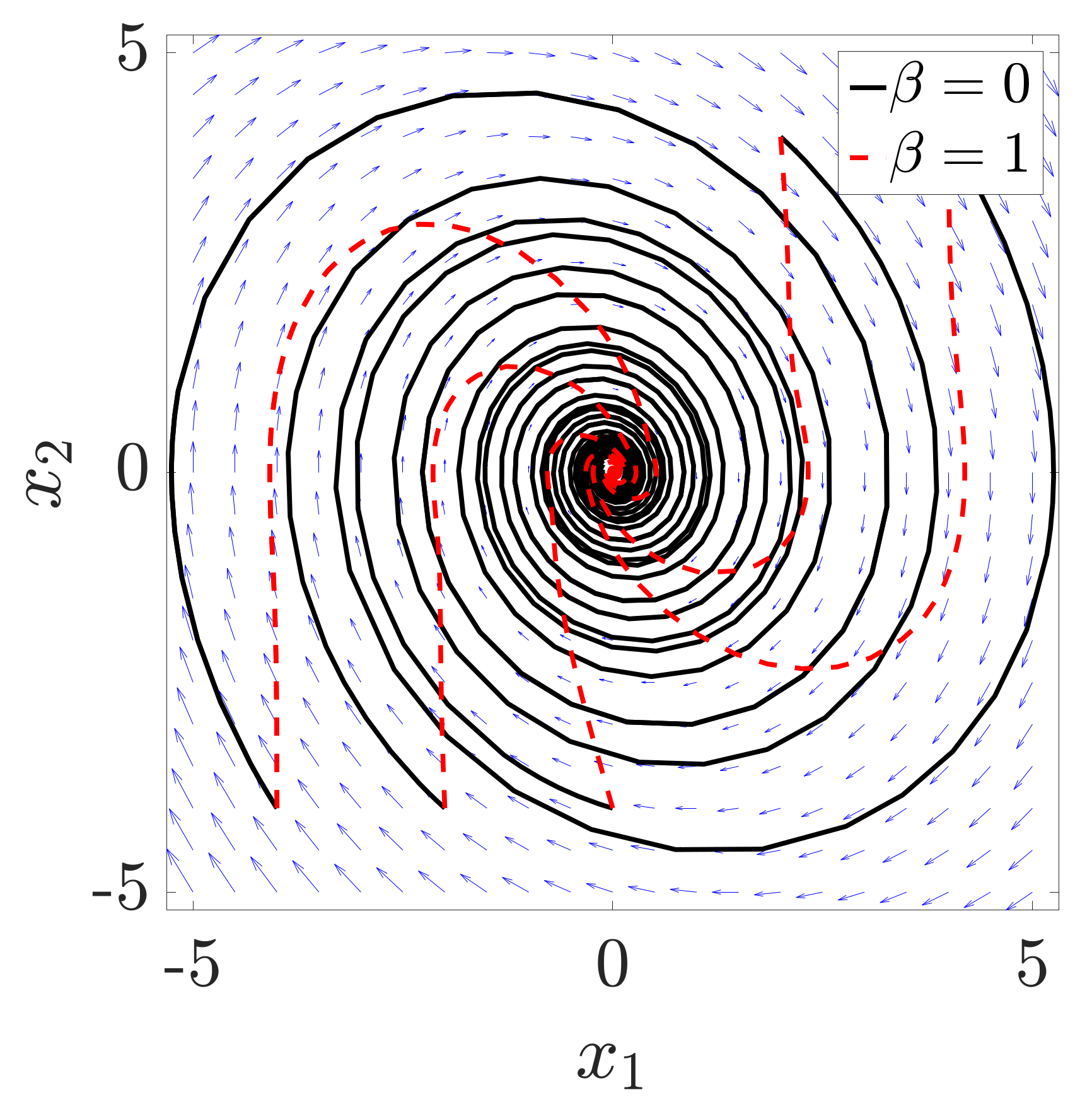
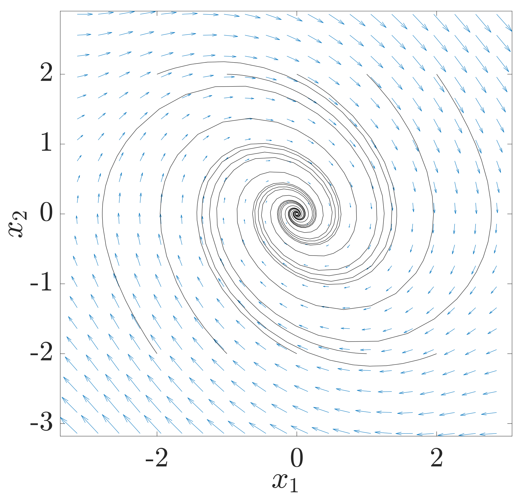
5.1. Van der Pol Oscillator

The dynamics of a Van der Pol Oscillator is [30]
x ˙ 1 = x 2 , x ˙ 2 = ( 1 x 1 2 ) x 2 x 1 + u .
We collect time-series data points for each input case by performing repeated simulations with time spans from 0 to 0.01 s and time step δ t = 0.01 s, starting from 2 × 10 4 random initial points in [ x 1 , x 2 ] = [ 5 , 5 ] 2 . The total data points for each input response case are T 0 = 19,952 , T 1 = 19,958 . The polynomial b ( x ) is chosen as an LQR solution associated with the linearized system at the origin. The value of α is set to be α = 4 . The optimization variables a ( x ) and c ( x ) are polynomials with degrees ranging from 0 to 2 and from 0 to 4, respectively. The basis Ψ ( x ) is chosen to be Legendre polynomials up to 15th order. Figure 1 shows the results of the control synthesized by following the proposed method described in Section 4 for β = 0 and β = 1 . Clearly, the case with geometric stable term ( β = 1 ) converges more aggressively to the origin.

5.2. Non-Polynomial System Example: Inverted Pendulum

The dynamics of a simple two-dimensional inverted pendulum is
x ˙ 1 = x 2 , x ˙ 2 = sin x 1 0.5 x 2 + u ,
which is non-polynomial due to a sinusoidal function. We collect time-series data points by performing repeated simulations, from 0 to 0.01 s with time step δ t = 0.01 s, starting from 10 4 random initial points from [ x 1 , x 2 ] = [ π , π ] 2 . The number of data points for both input response cases is T 0 = T 1 = 9989 . The value of α is set to be α = 4 . The polynomial b ( x ) is an LQR solution associated with the linearized system at the origin. The optimization variables a ( x ) and c ( x ) are polynomials with degrees from 0 to 2 and from 0 to 6, respectively. The basis Ψ ( x ) consists of monomials up to the 10th order. Figure 2 shows the results of the synthesized control for β = 0 and β = 7 , demonstrating that the control solutions from the proposed method can effectively stabilize non-polynomial dynamical systems, and this is also the case with geometric stable term ( β = 7 ), which can stabilize the system more aggressively.

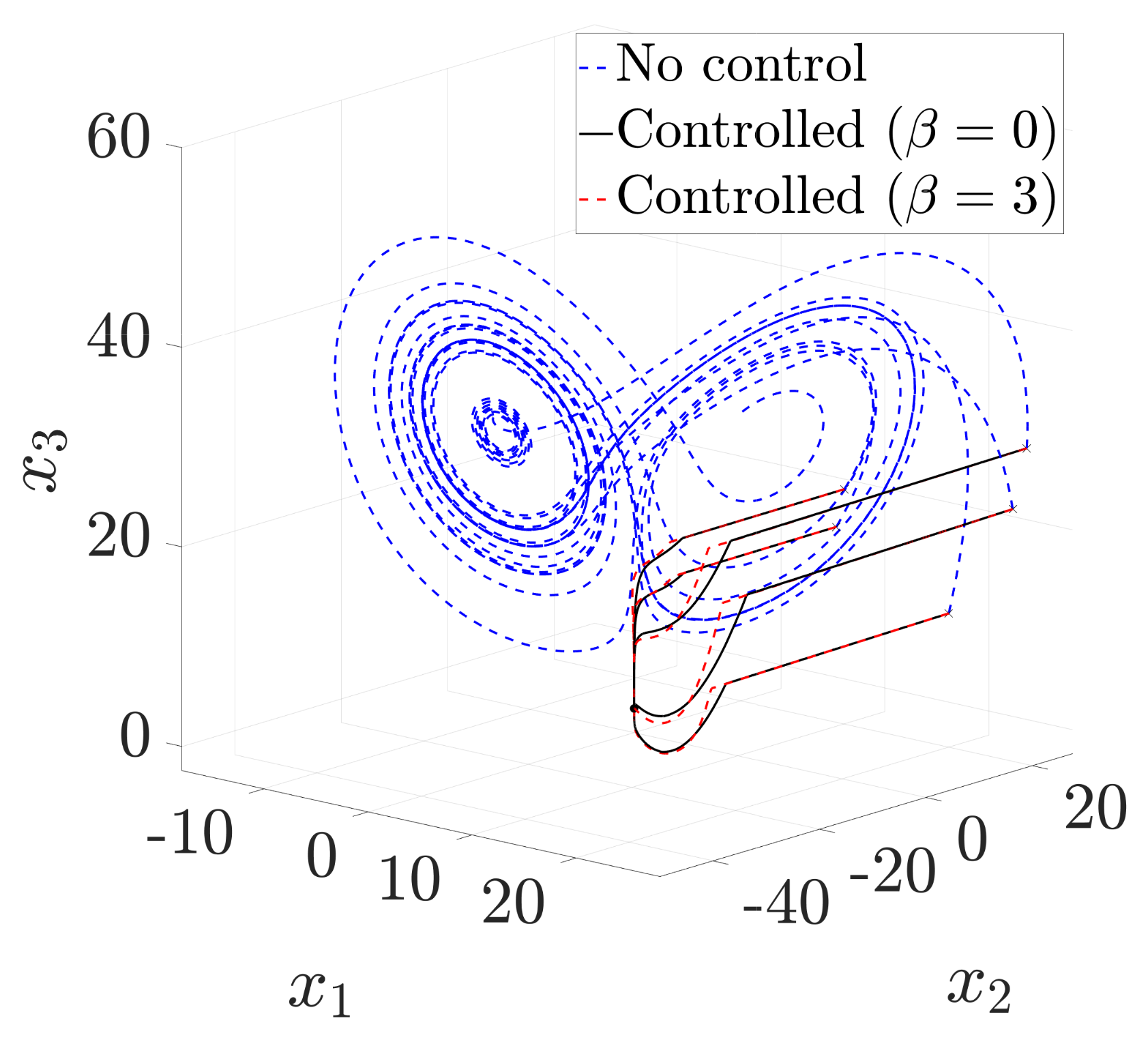
5.3. Lorenz System Dynamics

The dynamics of Lorenz attractor is given by [26]
x ˙ 1 = σ 1 ( x 2 x 1 ) , x ˙ 2 = x 1 ( σ 2 x 3 ) x 2 + u , x ˙ 3 = x 1 x 2 σ 3 x 3 ,
where the parameters are set to be σ 1 = 10 , σ 2 = 28 , and σ 3 = 8 3 . We collect time-series data points from repeated simulations, from 0 to 0.001 s, with time step δ t = 0.001 s, starting from random initial points in [ x 1 , x 2 , x 3 ] = [ 5 × 5 ] 3 . The data points collected for all input cases have T 0 = T 1 = 9949 snapshots. For the parameters of stability conditions, we choose α = 4 and b ( x ) to be the LQR solution for the linearized system. The optimization variables a ( x ) and c ( x ) are polynomials with degrees ranging from 0 to 2 and from 0 to 6, respectively. The basis Ψ ( x ) consists of Legendre polynomials up to the 10th order. Figure 3 shows the results of the synthesized controls for β = 0 and β = 3 . We can observe that the chaotic dynamics of the Lorenz attractor is stabilized to the origin by the control synthesized by our proposed method, and furthermore, the geometric stable term ( β = 3 ) stabilizes the system more aggressively.

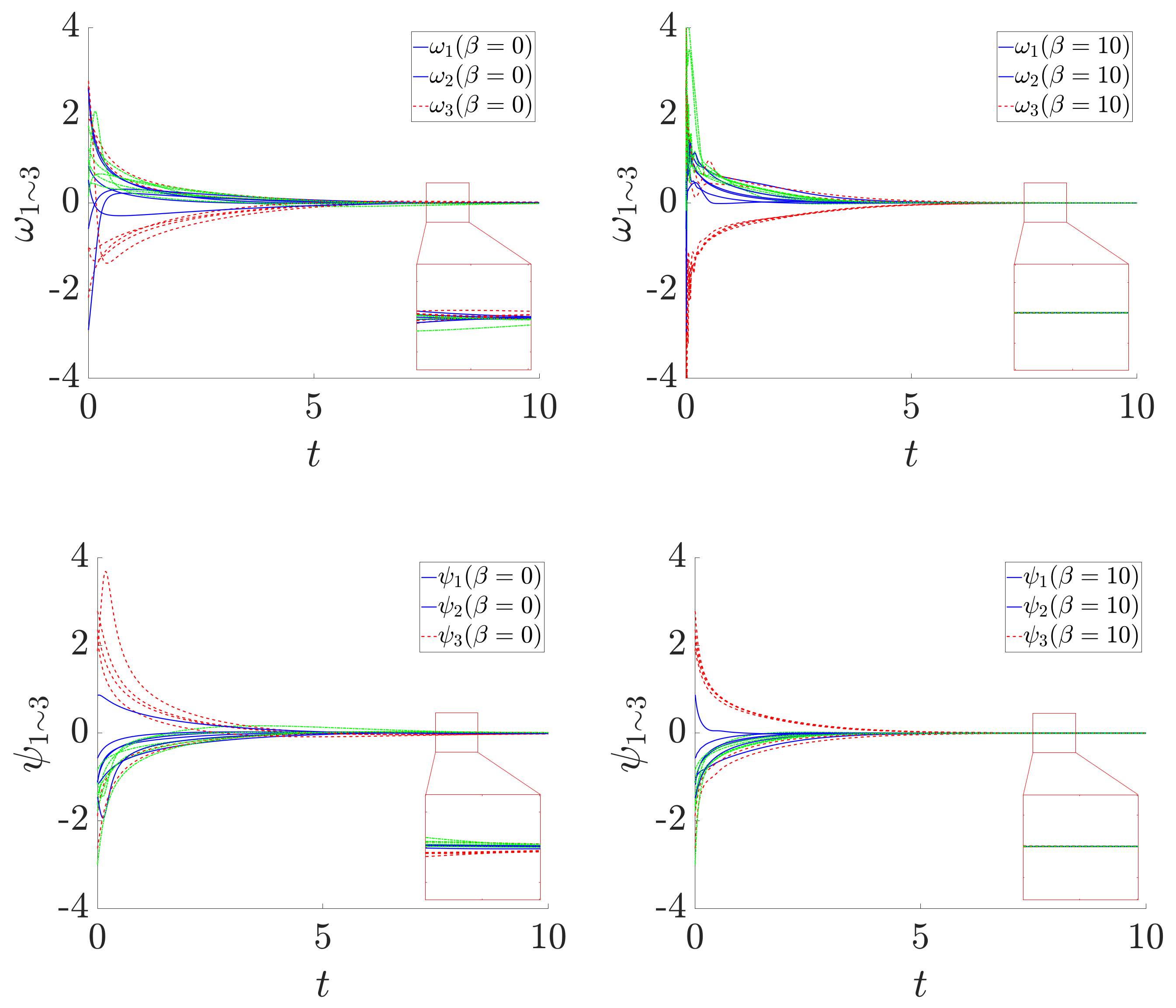
5.4. Rigid Body Control

Consider a rigid body system [25]
ω ˙ = J 1 S ( ω ) J ω + J 1 u , ψ ˙ = H ( ψ ) ω ,
where the angular velocity vector ω R 3 , Rodrigues parameter vector ψ R 3 , and control torque u R 3 . The explicit form of the parameters can be found in [25]. The dimension of the state space is 6. Time-series data points are sampled from repeated simulations with a time span from 0 to 0.001 s with time step δ t = 0.001 s, starting from uniformly distributed random initial points, [ ω , ψ ] = [ 3 × 3 ] 6 . Each data matrix, X 1 4 , X ˙ 1 4 has 9990 snapshots. The value of α is set to be α = 4 . The polynomial b is chosen to be b ( x ) = | ω + ψ | 2 + | ψ | 2 , which is known to be a CLF of the linearized dynamics of (38) from [25]. Degrees of a ( x ) = 1 and c j ( x ) are chosen to be from 0 to 1 and from 0 to 4, respectively. Figure 4 shows the trajectories of the states ω 1 3 and ψ 1 3 starting from some random initial points, stabilized by the proposed method for β = 0 (left) and β = 10 (right). Clearly, the case with β = 10 has a faster convergence property.

6. Concluding Remark

A systematic convex optimization-based framework is provided for the data-driven stabilization of control-affine nonlinear systems. The proposed approach relies on a combination of SOS optimization methods and recent advances in the data-driven computation of the Koopman operator. Future research efforts will focus on data-driven optimal control of the nonlinear system and the robust counterpart of this work by exploiting the sample complexity of Koopman and P-F operators [31].

Author Contributions

Conceptualization, U.V. and Y.C.; methodology, U.V. and Y.C.; investigation, H.C.; writing, H.C., U.V., and Y.C. All authors have read and agreed to the published version of the manuscript.

Funding

This work was partially supported by NSF under grant 1932458, 1901599 and 1942523, and DOE DE-OE-0000876.

Institutional Review Board Statement

Not applicable.

Informed Consent Statement

Not applicable.

Acknowledgments

H. Choi gratefully acknowledges funding from the Department of Energy, Office of Electricity’s Energy Storage Program, under the direction of Imre Gyuk. Sandia National Laboratories is a multi-mission laboratory managed and operated by National Technology and Engineering Solutions of Sandia, LLC., a wholly owned subsidiary of Honeywell International, Inc., for the U.S. Department of Energy’s National Nuclear Security Administration under contract DE-NA0003525. This paper describes objective technical results and analysis. Any subjective views or opinions that might be expressed in the paper do not necessarily represent the views of the U.S. Department of Energy or the United States Government.

Conflicts of Interest

The authors declare no conflict of interest.

References

  1. Rantzer, A. A dual to Lyapunov’s stability theorem. Syst. Control Lett. 2001, 42, 161–168. [Google Scholar] [CrossRef]
  2. Vaidya, U.; Mehta, P.G. Lyapunov measure for almost everywhere stability. IEEE Trans. Autom. Control 2008, 53, 307–323. [Google Scholar] [CrossRef]
  3. Rajaram, R.; Vaidya, U.; Fardad, M.; Ganapathysubramanian, B. Stability in the almost everywhere sense: A linear transfer operator approach. J. Math. Anal. Appl. 2010, 368, 144–156. [Google Scholar] [CrossRef] [Green Version]
  4. Das, A.K.; Huang, B.; Vaidya, U. Data-Driven Optimal Control Using Transfer Operators. In Proceedings of the IEEE Conference on Decision and Control (CDC), Miami, FL, USA, 17–19 December 2018; pp. 3223–3228. [Google Scholar]
  5. Raghunathan, A.; Vaidya, U. Optimal stabilization using Lyapunov measures. IEEE Trans. Autom. Control 2013, 59, 1316–1321. [Google Scholar] [CrossRef] [Green Version]
  6. Williams, M.O.; Kevrekidis, I.G.; Rowley, C.W. A Data-Driven Approximation of the Koopman Operator: Extending Dynamic Mode Decomposition. J. Nonlinear Sci. 2015, 25, 1307–1346. [Google Scholar] [CrossRef] [Green Version]
  7. Mezić, I. Analysis of Fluid Flows via Spectral Properties of the Koopman Operator. Annu. Rev. Fluid Mech. 2013, 45, 357–378. [Google Scholar] [CrossRef] [Green Version]
  8. Susuki, Y.; Mezic, I.; Raak, F.; Hikihara, T. Applied Koopman operator theory for power systems technology. Nonlinear Theory Its Appl. IEICE 2016, 7, 430–459. [Google Scholar] [CrossRef] [Green Version]
  9. Sharma, P.; Huang, B.; Ajjarapu, V.; Vaidya, U. Data-driven Identification and Prediction of Power System Dynamics Using Linear Operators. In Proceedings of the 2019 IEEE Power Energy Society General Meeting (PESGM), Atlanta, GA, USA, 4–8 August 2019; pp. 1–5. [Google Scholar]
  10. Mauroy, A.; Mezić, I. Global stability analysis using the eigenfunctions of the Koopman operator. IEEE Trans. Autom. Control 2016, 61, 3356–3369. [Google Scholar] [CrossRef] [Green Version]
  11. Korda, M.; Mezić, I. Linear predictors for nonlinear dynamical systems: Koopman operator meets model predictive control. Automatica 2018, 93, 149–160. [Google Scholar] [CrossRef] [Green Version]
  12. Huang, B.; Ma, X.; Vaidya, U. Data-driven nonlinear stabilization using koopman operator. In The Koopman Operator in Systems and Control; Springer: Berlin/Heidelberg, Germany, 2020; pp. 313–334. [Google Scholar]
  13. Kaiser, E.; Kutz, J.N.; Brunton, S.L. Data-driven discovery of Koopman eigenfunctions for control. arXiv 2017, arXiv:1707.01146. [Google Scholar]
  14. Kaiser, E.; Kutz, J.N.; Brunton, S.L. Data-Driven Approximations of Dynamical Systems Operators for Control; Springer: Heidelberg, Germany, 2020. [Google Scholar]
  15. Guo, M.; De Persis, C.; Tesi, P. Learning control for polynomial systems using sum of squares relaxations. In Proceedings of the 2020 59th IEEE Conference on Decision and Control (CDC), Jeju, Korea, 14–18 December 2020; pp. 2436–2441. [Google Scholar]
  16. Dai, T.; Sznaier, M. A semi-algebraic optimization approach to data-driven control of continuous-time nonlinear systems. IEEE Control Syst. Lett. 2020, 5, 487–492. [Google Scholar] [CrossRef]
  17. Zhao, P.; Mohan, S.; Vasudevan, R. Control synthesis for nonlinear optimal control via convex relaxations. In Proceedings of the 2017 American Control Conference (ACC), Seattle, WA, USA, 24–26 May 2017; pp. 2654–2661. [Google Scholar]
  18. Topcu, U.; Packard, A.; Seiler, P.; Balas, G. Help on SOS [Ask the Experts]. IEEE Control Syst. Mag. 2010, 30, 18–23. [Google Scholar]
  19. Parrilo, P.A. Semidefinite programming relaxations for semialgebraic problems. Math. Program. 2003, 96, 293–320. [Google Scholar] [CrossRef]
  20. Parrilo, P.A.; Sturmfels, B. Minimizing Polynomial Functions. Algorithmic Quantit. Real Algeb. Geom. 2003, 60, 83–99. [Google Scholar]
  21. Parrilo, P.A. Structured Semidefinite Programs and Semialgebraic Geometry Methods in Robustness and Optimization. Ph.D. Thesis, California Institute of Technology, Pasadena, CA, USA, 2000. [Google Scholar]
  22. Laurent, M. Sums of Squares, Moment Matrices and Optimization Over Polynomials. In Emerging Applications of Algebraic Geometry; Putinar, M., Sullivant, S., Eds.; Springer: New York, NY, USA, 2009; pp. 157–270. [Google Scholar]
  23. Papachristodoulou, A.; Anderson, J.; Valmorbida, G.; Prajna, S.; Seiler, P.; Parrilo, P.A. SOSTOOLS: Sum of Squares Optimization Toolbox for MATLAB. arXiv 2013, arXiv:1310.4716. [Google Scholar]
  24. Seiler, P. SOSOPT: A Toolbox for Polynomial Optimization. arXiv 2013, arXiv:1308.1889. [Google Scholar]
  25. Prajna, S.; Parrilo, P.A.; Rantzer, A. Nonlinear control synthesis by convex optimization. IEEE Trans. Autom. Control 2004, 49, 310–314. [Google Scholar] [CrossRef] [Green Version]
  26. Huang, B.; Ma, X.; Vaidya, U. Feedback Stabilization Using Koopman Operator. In Proceedings of the 2018 IEEE Conference on Decision and Control (CDC), Miami, FL, USA, 17–19 December 2018; pp. 6434–6439. [Google Scholar]
  27. Klus, S.; Nüske, F.; Peitz, S.; Niemann, J.H.; Clementi, C.; Schütte, C. Data-Driven Approximation of the Koopman Generator: Model Reduction, System Identification, and Control. Phys. D Nonlinear Phenom. 2020, 406, 132416. [Google Scholar] [CrossRef] [Green Version]
  28. Chartrand, R. Numerical Differentiation of Noisy, Nonsmooth Data. ISRN Appl. Math. 2011, 149–165. [Google Scholar] [CrossRef] [Green Version]
  29. Na, T. Computational Methods in Engineering Boundary Value Problems; Mathematics in Science and Engineering: A Series of Monographs and Textbooks; Academic Press: Cambridge, MA, USA, 1979. [Google Scholar]
  30. Ma, X.; Huang, B.; Vaidya, U. Optimal Quadratic Regulation of Nonlinear System Using Koopman Operator. In Proceedings of the 2019 American Control Conference (ACC), Philadelphia, PA, USA, 10–12 July 2019; pp. 4911–4916. [Google Scholar] [CrossRef]
  31. Chen, Y.; Vaidya, U. Sample Complexity for Nonlinear Stochastic Dynamics. In Proceedings of the 2019 American Control Conference (ACC), Philadelphia, PA, USA, 10–12 July 2019; pp. 3526–3531. [Google Scholar]
Figure 1. Van der Pol dynamics stabilized by proposed method.
Mathematics 09 02445 g001
Figure 2. Pendulum dynamics stabilized by proposed method.
Mathematics 09 02445 g002
Figure 3. Lorenz dynamics stabilized by proposed method.
Mathematics 09 02445 g003
Figure 4. Rigid body system stabilized by our proposed method.
Mathematics 09 02445 g004
Publisher’s Note: MDPI stays neutral with regard to jurisdictional claims in published maps and institutional affiliations.

