Global Stabilization of a Single-Species Ecosystem with Markovian Jumping under Neumann Boundary Value via Laplacian Semigroup

Abstract

By applying impulsive control, this work investigated the global stabilization of a single-species ecosystem with Markovian jumping, a time delay and a Neumann boundary condition. Variational methods, a fixed-point theorem, and Laplacian semigroup theory were employed to derive the unique existence of the global stable equilibrium point, which is a positive number. Numerical examples illuminate the feasibility of the proposed methods.

1. Introduction

As pointed out in [1], the following logistic system has been widely discussed and studied due to its importance in the development of ecology:

$$\frac{d\mathfrak{Z}}{dt}=-\mathfrak{R}(\frac{\mathfrak{Z}\left(t\right)}{\mathfrak{K}}-1)\mathfrak{Z}\left(t\right).$$

(1)

Here, $\mathfrak{Z}\left(t\right)$ is the population’s quantity or density at the time t, and $\mathfrak{K}$ and $\mathfrak{R}>0$ are the intrinsic growth rate of the environmental capacity and the population. Because all the solutions of nonlinear ecosystems are difficult to provide accurately, people pay more attention to the long-term dynamic trend of an ecosystem, i.e., the long-term trend of population density (see, for example, [1,2,3,4,5]). People especially want to know whether the population will tend to a positive constant after a long time, which is related to the final long-term existence of the population. For example, the long-term behavior of the following random single-species ecosystem was studied in [2]:

$$d\mathfrak{Z}=\gamma \mathfrak{Z}dB(t)-\mathfrak{Z}[b\mathfrak{Z}-a]dt.$$

(2)

Animal populations will inevitably spread because of climate, foraging and random walking. Hence, the reaction–diffusion ecological models well simulate a real ecosystem. Particularly, reaction–diffusion ecosystems were studied in [6,7]. For example, in [8], a single-species Markovian jumping ecosystem with diffusion and delayed feedback under a Dirichlet boundary value was investigated:

$$\left\{\begin{array}{cc}\hfill \frac{\partial v(t,x)}{\partial t}=& [a-bv(t,x)]v(t,x)+q\Delta v(t,x)-c(r(t))[v(t-\tau (t),x)-v(t,x)],x\in \mathrm{\Omega },t⩾0,\hfill \\ \hfill v(t,x)=& 0,t⩾0,x\in \partial \mathrm{\Omega }.\hfill \end{array}\right.$$

(3)

Markov systems often occur in various engineering technologies (see, for example, [9,10,11]). Particularly, a Markovian jumping delayed feedback model well reflects the influence of stochastic factors on time delays in the changes of populations, such as weather, temperature, humidity, ventilation status, etc. However, the case of a single-species ecosystem with a Neumann boundary value is seldom researched. In fact, a Neumann zero boundary value model well simulates the biosphere boundary without population migration. For example, freshwater fish do not enter the sea through rivers. Inspired by some ideas or methods of the related literature [6,7,8,9,10,11,12,13,14,15,16,17,18,19,20,21,22,23,24,25,26,27,28,29,30,31,32,33,34], we are willing to study the global stabilization of a Markovian jumping delayed feedback diffusion ecosystem with a single species equipped with the Neumann zero boundary value.

The main contributions are as follows.

• The uniqueness proof of the positive equilibrium solution is presented in this paper, while it was given in previous work that only involved the existence of the positive equilibrium solution.
• In the case of a single-species ecosystem with impulses, it is the first study using a Laplacian semigroup to globally stabilize the ecosystem.
• A numerical example is designed to illuminate the advantages of Theorem 2 against [22] (Theorem 4.2), as a result of reducing the algorithm’s conservatism.

For the sake of simplicity, we denote, by $\mathrm{\Omega }\subset R^N(1⩽N⩽3)$, a bounded domain, and $\partial \mathrm{\Omega }$ is its smooth boundary. Denote by $\overline{\mathrm{\Omega }}$ the closure of $\mathrm{\Omega }$, i.e., $\mathrm{\Omega }\bigcup \partial \Omega =\overline{\mathrm{\Omega }}$. ${\parallel \phi \parallel }_H=\sqrt{{\int }_{\mathrm{\Omega }}{|\nabla \phi (x)|}^{2}dx}$ represents the norm of the Sobolev space $H_0^1(\mathrm{\Omega })$. ${\lambda }_1$ represents the minimum positive eigenvalue of $-\Delta$ in the Sobolev space $H_0^1(\mathrm{\Omega }).$ In addition, for a vector $v={(v_1,v_2)}^T$, denote $|v|=(|v_1|,|v_2{|)}^T$, and for a matrix $A=(a_{ij})$, denote $|A|=(|a_{ij}|).$ Denote by $\mathbb{N}$ the natural numbers set. $L^2(\mathrm{\Omega })=\{f:{\int }_{\mathrm{\Omega }}{f}^2(x)dx<\infty \}$ is the real-valued functions space with the inner product $\langle f,g\rangle ={\int }_{\mathrm{\Omega }}f(x)g(x)dx,$ for $f,g\in L^2(\mathrm{\Omega })$, and its norm $\parallel f\parallel ={({\int }_{\mathrm{\Omega }}{f}^2(x)dx)}^{\frac{1}{2}}$ for $f\in L^2(\mathrm{\Omega }).$ The Laplace operator $\Delta =\sum _{j=1}^m\frac{{\partial }^2}{\partial x_j^2}$ and the semigroup $e^{t\Delta }$ can be seen in [35] in detail, for fear of repetition. $(\mathrm{{\rm Y}},\mathcal{F},\mathbb{P})$ is the probability space described in [8]. $S=\{1,2,\cdots ,n_0\}$, $\{r(t):[0,+\infty )\to S\}$, $\mathrm{\Pi }={({\gamma }_{ij})}_{n_0\times n_0}$ and the following formula are also the same as those of [8],

$$\mathbb{P}(j=r(t+\delta )\mid m=r(t))=\left\{\begin{array}{c}o(\delta )+{\gamma }_{mj}^{\delta ,}j\ne m\hfill \\ o(\delta )+1+{\gamma }_{mj}^{\delta ,}j=m,\hfill \end{array}\right.$$

(4)

2. Preparatory Work

Consider the reaction–diffusion delayed ecosystem:

$$\left\{\begin{array}{cc}\hfill \frac{\partial u(t,x)}{\partial t}=& [a-bu(t,x)]u(t,x)-[u(t,x)-u(t-\tau (t),x)]c(r(t))+q\Delta u(t,x),t⩾0,x\in \mathrm{\Omega },\hfill \\ \hfill 0=& \frac{\partial u(t,x)}{\partial x},t⩾0,x\in \partial \mathrm{\Omega },\hfill \\ \hfill \Gamma (s,x)=& u(s,x),(s,x)\in [-\tau ,0]\times \mathrm{\Omega }.\hfill \end{array}\right.$$

(5)

Here, $u(t,x)$ is the population density at time t and space point x. $a>0$ and $b>0$ are described similarly as those of [8]. $\tau (t)\in [0,\tau ]$, and $\Gamma (s,x)$ is the bounded initial value function on $[-\tau ,0]\times \mathrm{\Omega }.$ For convenience, $c(r(t))$ is denoted simply by $c_r$ for $r(t)=r\in S.$

In addition, due to the limited resources of nature, the population density should have an upper limit. At the same time, the population density should also have a lower limit because a low population density does not allow male and female animals to meet in the vast biosphere and reproduce.

Hypothesis 1 (H1).

There exist two positive constants$N_1$and$N_2$and a decimal$k_0\in (0,1)$with$(1+k_0)N_1⩽\frac{a}{b}⩽(1-k_0)N_2$and$(1+k_0)N_1⩽\Gamma (s,x)⩽(1-k_0)N_2$for$s\in [-\tau ,0],x\in \mathrm{\Omega }$, such that

$$0<N_1⩽u(t,x)⩽N_2,\forall x\in \overline{\mathrm{\Omega }},t⩾-\tau .$$

(6)

Remark 1.

The boundedness assumption in (H1) brings innovations. It ensures that the initial value maintains a certain distance from the upper and lower bounds, so that an impulse with an appropriate frequency and intensity can ensure that the dynamic behavior of the system with such an initial value will not exceed the bounds.

Definition 1.

$u_{*}(x)$ is a stationary solution of the system (5) i, f for $(t,x)\in [-\tau ,+\infty )\times \overline{\mathrm{\Omega }}$, $u_{*}(t,x)\equiv u_{*}(x)$, and $u_{*}(x)$ satisfies (H1), and

$$\left\{\begin{array}{c}[a-b{u}_{*}(x)]u_{*}(x)+q\Delta u_{*}(x)=0,x\in \mathrm{\Omega },t⩾0,\hfill \\ 0=\frac{\partial u_{*}(x)}{\partial x},t⩾0,x\in \partial \mathrm{\Omega }.\hfill \end{array}\right.$$

(7)

Now, it is easy to conclude from Definition 1 that $u_{*}\equiv \frac{a}{b}$ is a stationary solution of the system (5). Moreover, letting $U(t,x)=u(t,x)-u_{*}$, the system (5) is translated into

$$\left\{\begin{array}{cc}\hfill \frac{\partial U(t,x)}{\partial t}=& -b{U}^2(t,x)-aU(t,x)-c_r[U(t,x)-U(t-\tau (t),x)]+q\Delta U(t,x),x\in \mathrm{\Omega },t⩾0,\hfill \\ \hfill 0=& \frac{\partial U(t,x)}{\partial x},t⩾0,x\in \partial \mathrm{\Omega },\hfill \\ \hfill U(s,x)=& -\frac{a}{b}+\Gamma (s,x),(x,s)\in \mathrm{\Omega }\times [-\tau ,0].\hfill \end{array}\right.$$

(8)

Here, the positive solution $u_{*}\equiv \frac{a}{b}$ of the ecosystem (5) corresponds to the zero solution of the system (8). Thus, the stabilization of the above-mentioned zero solution will be investigated below. Furthermore, employing an impulse control on the natural ecosystem (5) or (8) results in

$$\left\{\begin{array}{cc}\hfill \frac{\partial U(t,x)}{\partial t}=& -b{U}^2(t,x)-aU(t,x)-c_r[U(t,x)-U(t-\tau (t),x)]+q\Delta U(t,x),t\ne t_k,t⩾0,x\in \mathrm{\Omega },\hfill \\ \hfill U(t^{+},x)=& M_{k}U(t^{-},x),t=t_k,k\in \mathbb{N},\hfill \\ \hfill 0=& \frac{\partial U(t,x)}{\partial x},x\in \partial \mathrm{\Omega },t⩾0,\hfill \\ \hfill U(s,x)=& -\frac{a}{b}+\Gamma (s,x)=\xi (s,x),(x,s)\in \mathrm{\Omega }\times [-\tau ,0],\hfill \end{array}\right.$$

(9)

whose zero solution corresponds to the stationary solution $u_{*}\equiv \frac{a}{b}$ of the following system:

$$\left\{\begin{array}{cc}\hfill \frac{\partial u(t,x)}{\partial t}=& -b{[u(t,x)-\frac{a}{b}]}^2-a[u(t,x)-\frac{a}{b}]-c_r[u(t,x)-u(t-\tau (t),x)]+q\Delta u(t,x),t⩾0,t\ne t_k,x\in \mathrm{\Omega },\hfill \\ \hfill u(t^{+},x)=& M_k[u(t^{-},x)-\frac{a}{b}]+\frac{a}{b},t=t_k,k\in \mathbb{N},\hfill \\ \hfill 0=& \frac{\partial u(t,x)}{\partial x},x\in \partial \mathrm{\Omega },t⩾0,\hfill \\ \hfill \Gamma (s,x)=& u(s,x),(x,s)\in \mathrm{\Omega }\times [-\tau ,0].\hfill \end{array}\right.$$

(10)

Here, we assume that $0<t_1<t_2<\cdots$, and each $t_k(k\in \mathbb{N})$ represents a fixed impulsive instant. Additionally, $\underset{t\to t_k^{+}}{lim}u(t,x)=u(t_k^{+},x)$, and $u(t_k^{-},x)=u(t_k,x)=\underset{t\to t_k^{-}}{lim}u(t,x)$.

Definition 2.

For any given $T>0,$ $U={\{U(t)\}}_{[0,T]}$ is an $L^2(\mathrm{\Omega })$-valued function, and it is called a mild solution of the system (9) if $U(t,x)\in \mathcal{C}([0,T];L^2(\mathrm{\Omega }))$ makes ${\int }_0^t{\parallel U_i(s)\parallel }^{p}ds<\infty ,i=1,2$ hold, and for any $t\in [0,T]$ and $x\in \mathrm{\Omega }$

$$\begin{array}{cc}\hfill U(t,x)=& e^{qt\Delta }\sum _{0<t_k<t}{e}^{-q{t}_k\Delta }(M_k-1)U(t_k,x)+{\int }_0^t{e}^{q(t-s)\Delta }\left(-b{U}^2(s,x)-aU(s,x)-c_r[U(s,x)-U(s-\tau (s),x)]\right)ds\hfill \\ & +e^{qt\Delta }\xi (0,x),t⩾0,\hfill \end{array}$$

(11)

and

$$\xi (s,x)=U(s,x),x\in \mathrm{\Omega },s\in [-\tau ,0],$$

$$0=\frac{\partial U}{\partial \nu },t⩾0,x\in \partial \mathrm{\Omega }.$$

Remark 2.

Definition 2 is well defined in view of [23,24]; particularly, the considerations about the impulsive items in [24] provide a useful hint for designing Definition 2.

In this paper, the following condition is also required:

Hypothesis 2 (H2).

There are two constants $M>0$ and $\gamma >0$ such that $\parallel e^{t\Delta }{\parallel }_2⩽M{e}^{-\gamma t}$, where $\parallel e^{t\Delta }{\parallel }_2=\underset{\parallel w\parallel =1}{sup}\parallel e^{t\Delta }w\parallel$ (see [23]).

Lemma 1.

(see, for example, [14]). $\mathrm{\Omega }\subset R^m$ is a bounded domain, and its smooth boundary $\partial \mathrm{\Omega }$ is of class ${\mathcal{C}}^2$. $\theta (x)\in H_0^1(\mathrm{\Omega })$ is a real-valued function, and $\frac{\partial \theta (x)}{\partial \nu }{|}_{\partial \mathrm{\Omega }}=0$. Then,

$${\int }_{\mathrm{\Omega }}{|\nabla \theta (x)|}^{2}dx⩾{\lambda }_1{\int }_{\mathrm{\Omega }}{|\theta (x)|}^{2}dx,$$

where ${\lambda }_1$ is the least positive eigenvalue of the following Neumann boundary problem:

$$\left\{\begin{array}{c}\lambda \theta -\Delta \theta =0,x\in \mathrm{\Omega },\hfill \\ \frac{\partial \theta (x)}{\partial \nu }=0,x\in \partial \mathrm{\Omega },\hfill \end{array}\right.$$

where ν is the external normal direction of $\partial \mathrm{\Omega }$.

Lemma 2.

([36]) If f is a contraction mapping on a complete metric space $\mathcal{H}$, there must exist a unique point $u\in \mathcal{H}$, satisfying $f(u)=u$.

3. Main Result

Firstly, the unique existence of the stationary solution of the ecosystem (5) should be considered. Moreover, the unique stationary solution of the ecosystem should be positive. Based on these two points, we present the following unique existence theorem:

Theorem 1.

Suppose (H1) holds. For all $r(t)=r\in S$, the system (5) possesses a positive stationary solution $u_{*}\equiv \frac{a}{b}$ for all $(t,x)\in [-\tau ,+\infty )\times \overline{\mathrm{\Omega }}$. If, in addition, the following condition is satisfied:

$$a<{\lambda }_{1}q+2b{N}_1$$

(12)

then the positive solution $u_{*}$ is the unique stationary solution of the system (5).

Proof. 

Obviously, for $(t,x)\in [-\tau ,0]\times \overline{\mathrm{\Omega }}$, $u_{*}\equiv \frac{a}{b}$ makes the following equations hold:

$$q\Delta u_{*}+u_{*}[a-b{u}_{*}]=0,t⩾0,x\in \mathrm{\Omega },$$

and

$$\frac{\partial u_{*}}{\partial x}=0,x\in \partial \mathrm{\Omega },t⩾0.$$

Thus, Definition 1 yields that $u_{*}>0$ defined in Theorem 1 is the unique stationary solution of the system (5).

Below, we claim that $u_{*}$ is the unique stationary solution of the ecosystem (5).

Indeed, if $u_{*}$ and $v_{*}(x)$ are two different stationary solutions of the system (5), then Poincare inequality and the boundary condition yield

$$a{\int }_{\mathrm{\Omega }}{(u_{*}-v_{*}(x))}^{2}dx-b{\int }_{\mathrm{\Omega }}{(u_{*}-v_{*}(x))}^2(u_{*}+v_{*}(x))dx⩾{\lambda }_{1}q{\int }_{\mathrm{\Omega }}{|u_{*}-v_{*}(x)|}^{2}dx.$$

(13)

The condition (12), Definition 2 and the continuity of $u_{*}$ and $v_{*}$ lead to

$$a{\int }_{\mathrm{\Omega }}{(u_{*}-v_{*}(x))}^{2}dx-b{\int }_{\mathrm{\Omega }}{(u_{*}-v_{*}(x))}^2(u_{*}+v_{*}(x))dx<{\lambda }_1{\int }_{\mathrm{\Omega }}{|u_{*}-v_{*}(x)|}^{2}dx,$$

which contradicts the inequality (13).

This completes the proof. □

Remark 3.

As far as our knowledge, Theorem 1 is the first theorem to provide the unique existence of the stationary solution of a single-species ecosystem under a Neumann boundary value.

Remark 4.

This paper provides the unique existence of a stationary solution of a reaction–diffusion system. However, there are many previous articles related to reaction–diffusion systems that only involve the existence of the equilibrium point. For example, in [14], only the unique existence of the constant equilibrium point of a reaction–diffusion system with a Neumann boundary value was given, but the stationary solutions of a reaction–diffusion system may include the non-constant stationary solutions. Because the solution $u(t,x)$ of a reaction–diffusion system involves not only the time variable t but also the space variable x, its stationary solution should be $u_{*}(x)$, independent of the time variable t. Obviously, $u_{*}(x)$ must not be a constant equilibrium point, which may be dependent upon the space variable x. Thereby, it is not inappropriate to prove that the equilibrium point is the unique constant equilibrium point in [14]. It must be proved that it is the unique stationary solution, just like that of this paper. A similar example can also be found in [12].

Note that the system (10) has the same elliptic equation as that of the system (5), and hence, each stationary solution of the system (5) is that of the system (10), and vice versa. i.e., Theorem 1 shows that $u_{*}\equiv \frac{a}{b}$ is also the unique stationary solution of the system (10). Next, the global stability of the stationary solution $u_{*}\equiv \frac{a}{b}$ should be investigated.

Theorem 2.

Set $p⩾1$. Suppose all the conditions of Theorem 1 hold. Assume, in addition, the condition (H2) holds, and

$$0<{\varpi }_r<1,r(t)=r\in \mathcal{S};$$

(14)

then, $u_{*}\equiv \frac{a}{b}$ of the system (10) is globally exponentially stable in the pth moment; equivalently, the null solution of the system (9) is globally exponentially stable in the pth moment, where $\mu =\underset{k\in \mathbb{N}}{inf}(t_{k+1}-t_k)>0,$ $N_0=max\{|N_1-\frac{a}{b}|,N_2-\frac{a}{b}\}$

$${\varpi }_r={\left[4^{p-1}\left(b{(\frac{2M{N}_0}{q\gamma })}^p+(a+c_r){(\frac{M}{q\gamma })}^p+c_r{(\frac{M}{q\gamma })}^p+M^{2p}(\underset{k}{max}|M_k-1{|)}^p{\left(1+\frac{1}{q\gamma \mu }\right)}^p\right)\right]}^{\frac{1}{p}}.$$

(15)

Proof. 

Let the normed space $\mathcal{H}$ be the functions space consisting of functions $g(t,x):[-\tau ,+\infty )\times \overline{\mathrm{\Omega }}\to [N_1-\frac{a}{b},N_2-\frac{a}{b}]$, where g satisfies:

• (A1) g is pth moment continuous at $t⩾0$ with $t\ne t_k(k\in \mathbb{N})$;
• (A2) for any given $x\in \mathrm{\Omega }$, $\underset{t\to t_k^{-}}{lim}g(t,x)$ and $\underset{t\to t_k^{+}}{lim}g(t,x)$ exist, and $\underset{t\to t_k^{-}}{lim}g(t,x)=g(t_k,x)$;
• (A3) $g(s,x)=\xi (s,x),\forall s\in [-\tau ,0],x\in \mathrm{\Omega }$;
• (A4) $e^{\alpha t}{\parallel g(t)\parallel }^p\to 0$ as $t\to +\infty$, where $\alpha$ is a positive scalar with $0<\alpha <q\gamma$.

It is easy to verify that $\mathcal{H}$ is a complete metric space equipped with the following distance:

$$\mathrm{dist}\left(U,V\right)={\left(\underset{t⩾-\tau }{sup}{\parallel U(t,x)-V(t,x)\parallel }^p\right)}^{\frac{1}{p}},\forall U,V\in \mathcal{H}.$$

(16)

Construct an operator $\mathcal{\Theta }$ such that, for any given $U\in \mathcal{H},$

$$\left\{\begin{array}{cc}\hfill \mathcal{\Theta }(U)(t,x)=& e^{qt\Delta }\sum _{0<t_k<t}{e}^{-q{t}_k\Delta }(M_k-1)U(t_k,x)+{\int }_0^t{e}^{q(t-s)\Delta }(-b{U}^2(s,x)-aU(s,x)-c_r[U(s,x)\hfill \\ & -U(s-\tau (s),x)])ds+e^{qt\Delta }\xi (0,x),t⩾0,\hfill \\ \hfill 0=& \frac{\partial \mathcal{\Theta }(U)}{\partial \nu },x\in \partial \mathrm{\Omega },t⩾0,\hfill \\ \hfill \xi (s,x)=& \mathcal{\Theta }(U)(s,x),s\in [-\tau ,0],x\in \mathrm{\Omega }.\hfill \end{array}\right.$$

(17)

Below, we want to prove that $\mathcal{\Theta }:\mathcal{H}\to \mathcal{H}$, and it takes four steps to achieve the goal.

Step 1. It is claimed that, for $U\in \mathcal{H}$, $\mathcal{\Theta }(U)$ must be pth moment continuous at $t⩾0$ with $t\ne t_k(k\in \mathbb{N})$.

Indeed, $U\in [N_1-\frac{a}{b},N_2-\frac{a}{b}]$ means the boundedness of U, and let $\delta$ be a scalar small enough; a routine proof yields that if $\delta \to 0,$ for $t\in [0,+\infty )\backslash {\{t_k\}}_{k=1}^{\infty }$,

$$\begin{array}{c}{\parallel \mathcal{\Theta }(U)(t,x)-\mathcal{\Theta }(U)(t+\delta ,x)\parallel }^p⩽4^{p-1}\parallel e^{qt\Delta }\xi (0,x)-e^{q(t+\delta )\Delta }{\xi (0,x)\parallel }^p\hfill \\ +4^{p-1}\parallel {\int }_0^t{e}^{q(t-s)\Delta }[-aU(s,x)-b{U}^2(s,x)]ds-{\int }_0^{t+\delta }{e}^{q(t+\delta -s)\Delta }[-aU(s,x)-b{U}^2(s,x)]{ds\parallel }^p\hfill \\ +4^{p-1}\parallel {\int }_0^t{e}^{q(t-s)\Delta }[c_r(U(s,x)-U(s-\tau (s),x))]ds-{\int }_0^{t+\delta }{e}^{q(t+\delta -s)\Delta }[c_r(U(s,x)-U(s-\tau (s),x))]{ds\parallel }^p\hfill \\ +4^{p-1}{\parallel e^{qt\Delta }\sum _{0<t_k<t}{e}^{-q{t}_k\Delta }(M_k-1)U(t_k,x)-e^{q(t+\delta )\Delta }\sum _{0<t_k<t+\delta }{e}^{-q{t}_k\Delta }(M_k-1)U(t_k,x)\parallel }^p\to 0,\hfill \end{array}$$

(18)

which proves the claim. Then, (A1) is verified.

Step 2. $\mathcal{\Theta }(U)$ satisfies (A2), where $U\in \mathcal{H}$.

In fact, for $U\in \mathcal{H}$, people can easily see from (17) that $\underset{t\to t_k^{+}}{lim}\mathcal{\Theta }(U)(t,x)$ and $\underset{t\to t_k^{-}}{lim}\mathcal{\Theta }(U)(t,x)$ exist, and $\mathcal{\Theta }(U)(t_k,x)=\underset{t\to t_k^{-}}{lim}\mathcal{\Theta }(U)(t,x)$, which verifies (A2).

Step 3. $\mathcal{\Theta }(U)$ satisfies (A3), where $U\in \mathcal{H}$. Indeed, the third equation of (17) verifies (A3) directly.

Step 4. Verifying (A4), i.e., for $U\in \mathcal{H}$, verifying

$$e^{\alpha t}\parallel \mathcal{\Theta }(U)(t){\parallel }^p\to 0,\mathrm{if}t\to +\infty .$$

(19)

Indeed,

$$\begin{array}{cc}& e^{\alpha t}{\parallel \mathcal{\Theta }(U)(t,x)\parallel }^p=e^{\alpha t}\parallel e^{qt\Delta }\xi (0,x)+{\int }_0^t{e}^{q(t-s)\Delta }\left(-aU(s,x)-b{U}^2(s,x)-c_r[U(s,x)-U(s-\tau (s),x)]\right)ds\hfill \\ & +e^{qt\Delta }\sum _{0<t_k<t}{e}^{-q{t}_k\Delta }(M_k-1)U(t_k,x){\parallel }^p\hfill \\ \hfill ⩽& 5^{p-1}{e}^{\alpha t}\parallel e^{qt\Delta }\xi (0,x){\parallel }^p+5^{p-1}{e}^{\alpha t}\parallel {\int }_0^t{e}^{q(t-s)\Delta }[-aU(s,x)-b{U}^2(s,x)]{ds\parallel }^p+5^{p-1}{e}^{\alpha t}\parallel {\int }_0^t{e}^{q(t-s)\Delta }{c}_{r}U(s,x){ds\parallel }^p\hfill \\ & +5^{p-1}{e}^{\alpha t}\parallel {\int }_0^t{e}^{q(t-s)\Delta }{c}_{r}U(s-\tau (s),x){ds\parallel }^p+5^{p-1}{e}^{\alpha t}{\parallel e^{qt\Delta }\sum _{0<t_k<t}{e}^{-q{t}_k\Delta }(M_k-1)U(t_k,x)\parallel }^p,t⩾0,\hfill \end{array}$$

(20)

Moreover,

$$e^{\alpha t}\parallel e^{qt\Delta }{\xi (0,x)\parallel }^p⩽M^p{e}^{\alpha t}{e}^{-\gamma qt}{\parallel \xi (0,x)\parallel }^p\to 0,\mathrm{if}t\to +\infty .$$

(21)

$U\in \mathcal{H}$ means $U\in [N_1-\frac{a}{b},N_2-\frac{a}{b}]$, and

$$U^2⩽N_0|U|,\mathrm{where}{N}_0=max\{|N_1-\frac{a}{b}|,N_2-\frac{a}{b}\}.$$

(22)

The Holder inequality yields

$$\begin{array}{cc}& e^{\alpha t}{\parallel {\int }_0^t{e}^{q(t-s)\Delta }\left(-aU(s,x)-b{U}^2(s,x)\right)ds\parallel }^p\hfill \\ \hfill ⩽& 2^{p-1}{M}^p\left[a^p{(\frac{1}{q\gamma })}^{p-1}{\int }_0^t{e}^{-(q\gamma -\alpha )(t-s)}{e}^{\alpha s}\parallel U(s,x){\parallel }^{p}ds+b^p{N}_0^p{(\frac{1}{q\gamma })}^{p-1}{\int }_0^t{e}^{-q\gamma (t-s)}{\parallel U\parallel }^{p}ds\right].\hfill \end{array}$$

(23)

On the other hard, $e^{\alpha t}{\parallel U_i(t)\parallel }^p\to 0$ means that, for any $\epsilon >0$, there exists $t^{*}>0$ such that all $e^{\alpha t}{\parallel U_i(t)\parallel }^p<\epsilon .$ Therefore,

$$\begin{array}{cc}& {\int }_0^t{e}^{-(q\gamma -\alpha )(t-s)}{e}^{\alpha s}{\parallel U(s,x)\parallel }^{p}ds\hfill \\ \hfill ⩽& \underset{s\in [0,t^{*}]}{max}(e^{\alpha s}{\parallel U(s,x)\parallel }^p)e^{-(q\gamma -\alpha )t}\frac{1}{q\gamma -\alpha }{e}^{(q\gamma -\alpha )t^{*}}+\epsilon \frac{1}{q\gamma -\alpha },\hfill \end{array}$$

which, together with the arbitrariness of $\epsilon$, means that

$${\int }_0^t{e}^{-(q\gamma -\alpha )(t-s)}{\parallel U(s,x)\parallel }^p{e}^{\alpha s}ds\to 0,t\to +\infty .$$

(24)

Now, similarly to the proof of (23), one can prove

$$e^{\alpha t}{\parallel {\int }_0^t{e}^{q(t-s)\Delta }[-aU(s,x)-b{U}^2(s,x)]ds\parallel }^p,t\to +\infty .$$

(25)

$$e^{\alpha t}{\parallel {\int }_0^t{e}^{q(t-s)\Delta }{c}_{r}U(s,x)ds\parallel }^p,,t\to +\infty .$$

(26)

Since $U(s,x)=\xi (s,x)$ is bounded on $[-\tau ,0]\times \mathrm{\Omega }$, it is not difficult to similarly prove

$$e^{\alpha t}{\parallel {\int }_0^t{e}^{q(t-s)\Delta }{c}_{r}U(s-\tau (s),x)ds\parallel }^p,t\to +\infty .$$

(27)

Next, using the definition of the Riemann integral ${\int }_a^b{e}^{s}ds$ results in

$$\begin{array}{cc}& e^{\alpha t}\parallel e^{qt\Delta }\sum _{0<t_k<t}{e}^{-q{t}_k\Delta }(M_k-1)U(t_k,x){\parallel }^p\hfill \\ \hfill ⩽& 2^{p-1}\underset{k}{max}|M_k-1|\left[e^{-(pq\gamma -\alpha )t}{\left(\sum _{0<t_k⩽t^{*}}{e}^{q\gamma t_k}\parallel U(t_k,x)\parallel \right)}^p+\epsilon \frac{1}{{(q\gamma -\frac{\alpha }{p})}^p}\right]\to 0.\hfill \end{array}$$

(28)

Combining (20)–(28) yields (19).

It follows from the above four steps that

$$\mathcal{\Theta }(\mathcal{H})\subset \mathcal{H}.$$

(29)

Finally, we claim that $\mathcal{\Theta }$ is a contractive mapping on $\mathcal{H}$.

Indeed, for any $U,V\in \mathcal{H}$, the Holder inequality and (H2) yield

$$\begin{array}{cc}& \parallel {\int }_0^t{e}^{q(t-s)\Delta }{[V(s,x)-U(s,x)]ds\parallel }^p\hfill \\ \hfill ⩽& {\left(M{\int }_0^t{e}^{-q\gamma (t-s)}\parallel V(s,x)-U(s,x)\parallel ds\right)}^p\hfill \\ \hfill ⩽& M^p{\left({(\frac{1}{q\gamma })}^{\frac{p-1}{p}}[\underset{t⩾-\tau }{sup}\parallel U(t,x)-V(t,x){{\parallel }^p]}^{\frac{1}{p}}{(\frac{1}{q\gamma })}^{\frac{1}{p}}\right)}^p\hfill \\ \hfill ⩽& {(\frac{M}{q\gamma })}^p{[\mathrm{dist}(U,V)]}^p.\hfill \end{array}$$

(30)

Similarly,

$$\begin{array}{cc}& \parallel {\int }_0^t{e}^{q(t-s)\Delta }[U^2(s,x)-V^2(s,x)]{ds\parallel }^p\hfill \\ \hfill ⩽& {\left(2M{N}_0{\int }_0^t{e}^{-q\gamma (t-s)}\parallel U(s,x)-V(s,x)\parallel ds\right)}^p\hfill \\ \hfill ⩽& {(\frac{2M{N}_0}{q\gamma })}^p{[\mathrm{dist}(U,V)]}^p,\hfill \end{array}$$

(31)

and

$$\parallel {\int }_0^t{e}^{q(t-s)\Delta }{[V(s-\tau (s),x)-U(s-\tau (s),x)]ds\parallel }^p⩽{(\frac{M}{q\gamma })}^p{[\mathrm{dist}(U,V)]}^p$$

(32)

Assume $t_{j-1}<t⩽t_j$; then, the definition of the Riemann integral ${\int }_a^b{e}^{s}ds$ yields

$$\begin{array}{cc}& \parallel e^{qt\Delta }\sum _{0<t_k<t}{e}^{-q{t}_k\Delta }(M_k-1)[U(t_k,x)-V(t_k,x)]{\parallel }^p\hfill \\ \hfill ⩽& M^{2p}(\underset{k}{max}|M_k-{1|)}^p{\left[e^{-q\gamma t}\left(e^{q\gamma t_{j-1}}+\frac{1}{\mu }\sum _{0<t_k⩽t_{j-2}}{e}^{q\gamma t_k}(t_{k+1}-t_k)\right)·\mathrm{dist}(U,V)\right]}^p\hfill \\ \hfill ⩽& M^{2p}(\underset{k}{max}|M_k-1{|)}^p{\left(1+\frac{1}{q\gamma \mu }\right)}^p·{[\mathrm{dist}(U,V)]}^p.\hfill \end{array}$$

(33)

It follows from (30)–(33) that

$$\begin{array}{cc}& {\parallel \mathcal{\Theta }(U)-\mathcal{\Theta }(V)\parallel }^p\hfill \\ \hfill ⩽& 4^{p-1}b\parallel {\int }_0^t{e}^{q(t-s)\Delta }[U^2(s,x)-V^2(s,x)]{ds\parallel }^p+4^{p-1}(a+c_r)\parallel {\int }_0^t{e}^{q(t-s)\Delta }[U(s,x)-V(s,x)]{ds\parallel }^p\hfill \\ & +4^{p-1}\parallel {\int }_0^t{e}^{q(t-s)\Delta }{e}^{qt\Delta }\sum _{0<t_k<t}{e}^{-q{t}_k\Delta }(M_k-1)[U(t_k,x)-V(t_k,x)]{\parallel }^p\hfill \\ & +4^{p-1}{c}_r{\parallel {\int }_0^t{e}^{q(t-s)\Delta }[U(s-\tau (s),x)-V(s-\tau (s),x)]ds\parallel }^p⩽\hfill \\ \hfill ⩽& 4^{p-1}{[\mathrm{dist}(U,V)]}^p\left((a+c_r){(\frac{M}{q\gamma })}^p+b{(\frac{2M{N}_0}{q\gamma })}^p+c_r{(\frac{M}{q\gamma })}^p+M^{2p}(\underset{k}{max}|M_k-1{|)}^p{\left(1+\frac{1}{q\gamma \mu }\right)}^p\right),\hfill \end{array}$$

which derives

$$\mathrm{dist}(\mathcal{\Theta }(V),\mathcal{\Theta }(U))⩽\mathrm{dist}(U,V)(\underset{r\in S}{max}{\varpi }_r),\forall U,V\in \mathcal{H}.$$

Now, the definition of ${\varpi }_r$ implies that $\mathcal{\Theta }:\mathcal{H}\to \mathcal{H}$ is contractive such that there must exist the fixed point U of $\mathcal{\Theta }$ in $\mathcal{H}$, which means that U is the solution of the system (9), satisfying $e^{\alpha t}\parallel U{\parallel }^p\to 0$, $t\to +\infty$ so that $e^{\alpha t}\parallel u-u_{*}{\parallel }^p\to 0$, $t\to +\infty$. Therefore, the zero solution of the system (9) is the globally exponential stability in the pth moment; equivalently, $u_{*}\equiv \frac{a}{b}$ of the system (10) is the globally exponential stability in the pth moment. □

Remark 5.

To the best of our knowledge, this is the first paper to employ impulsive control and the Laplacian semigroup to globally stabilize a single-species ecosystem.

Remark 6.

This paper reports the global stability of a single-species ecosystem, while the stability in [3] did not involve the global one. This means that the stability in [3] depends heavily on the choice of initial value, while the global stability does not need such a choice. On the other hand, Equation (5) involves the space state, while the models in [3] did not involve the spatial location. In fact, population migration has a great impact on population stability, so the spatial state should be considered in the ecosystem model.

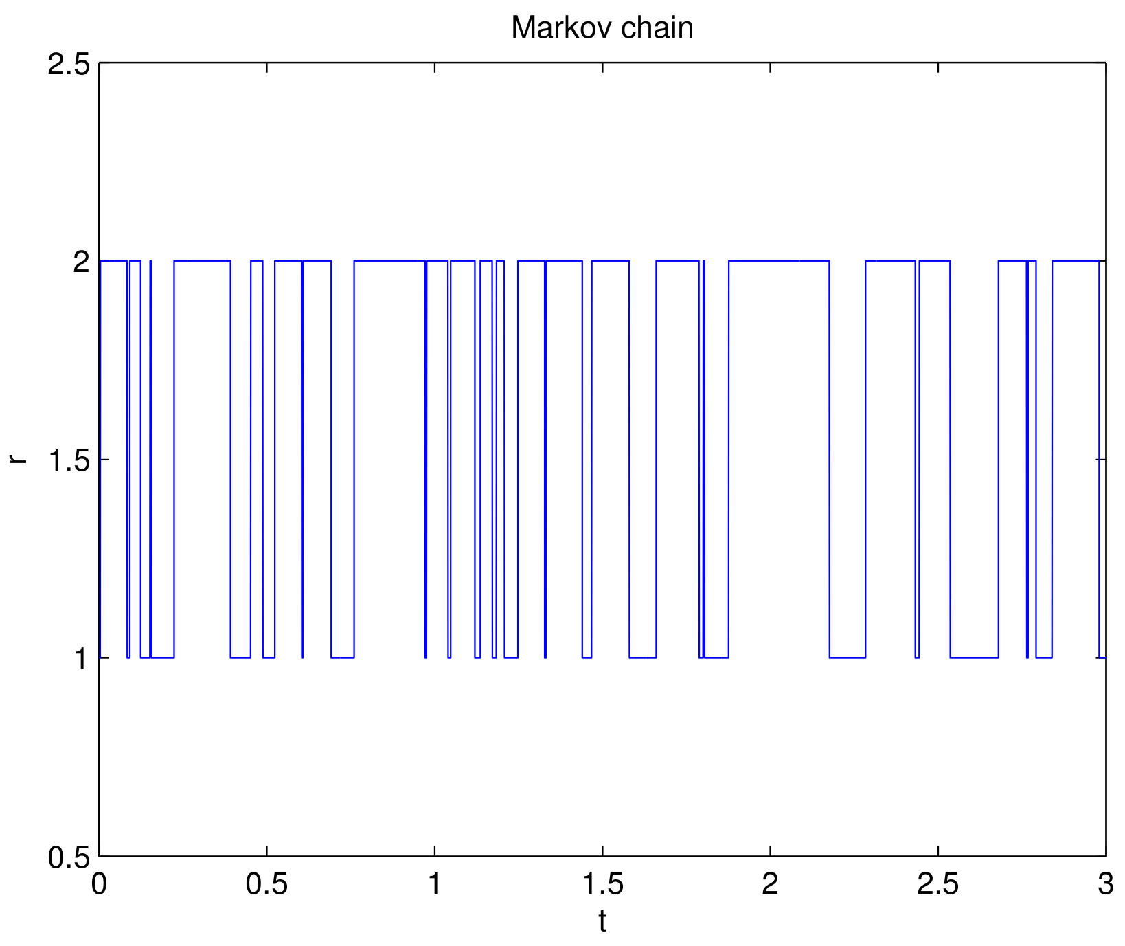
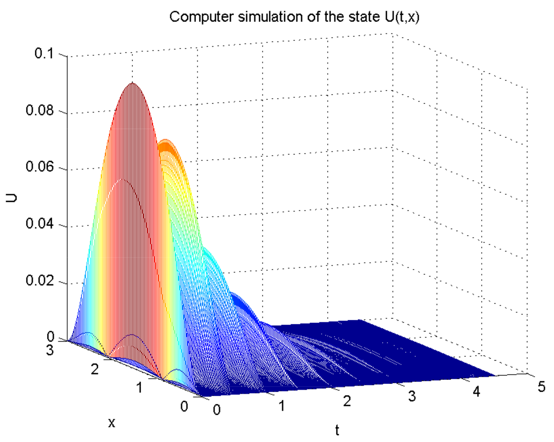
4. Numerical Example

Example 1.

Set $S=\{1,2\}$, $c_1=0.03,c_2=0.06,{\gamma }_{11}=-0.23,{\gamma }_{12}=0.23,{\gamma }_{21}=0.16,$ and ${\gamma }_{22}=-0.16$. Assume $\Gamma (s,x)\equiv 0.453,$$q=0.2,a=0.1692,b=0.4,N_1=0.3,and{N}_2=0.523,$; then, $N_0=0.123,u_{*}=0.423.$ Suppose, in addition, $\mathrm{\Omega }=(0,\pi ),$$\tau =0.5\equiv \tau (t)$ for all $t⩾0.$ Then, by computing the eigenfunctions of $-\Delta$, one can obtain $\parallel e^{t\Delta }\parallel ⩽e^{-{\pi }^{2}t},t⩾0$, and so $\gamma ={\pi }^2={\lambda }_1,M=1.$ Direct computation yields

$$0.1692=a<2.2139={\lambda }_{1}q+2b{N}_1,$$

which implies that the condition (12) is satisfied. Let $k_0=0.001,$ and obviously, the condition (H1) holds. Theorem 1 yields that the positive solution $u_{*}\equiv 0.423$ is the unique stationary solution of the system (5).

Example 2.

This example uses all the data provided in Example 1. Assume, in addition, $p=1.005,M_k\equiv 1.02,\mu =5$; obviously, the condition (H2) holds in Example 1. Moreover, we can obtain, by direct calculations, that

$$0<{\varpi }_1={\left[4^{p-1}\left((a+c_1){(\frac{M}{q\gamma })}^p+b{(\frac{2M{N}_0}{q\gamma })}^p+c_1{(\frac{M}{q\gamma })}^p+M^{2p}(\underset{k}{max}|M_k-1{|)}^p{\left(1+\frac{1}{q\gamma \mu }\right)}^p\right)\right]}^{\frac{1}{p}}<1,$$

and

$$0<{\varpi }_2={\left[4^{p-1}\left((a+c_2){(\frac{M}{q\gamma })}^p+b{(\frac{2M{N}_0}{q\gamma })}^p+c_2{(\frac{M}{q\gamma })}^p+M^{2p}(\underset{k}{max}|M_k-1{|)}^p{\left(1+\frac{1}{q\gamma \mu }\right)}^p\right)\right]}^{\frac{1}{p}}<1.$$

and, hence, the condition (14) is satisfied.

Thereby, Theorem 2 yields that the null solution of the system (9) is globally exponentially stable in the pth moment; equivalently, $u_{*}\equiv 0.423$ of the system (10) is globally exponentially stable in the pth moment (see Figure 1 and Figure 2).

Remark 7.

Obviously, Example 2 illuminates that Theorem 2 is better than [22] (Theorem 4.2) due to reducing the conservatism of the algorithm, because the pulse intensity in Theorem 2 does not require the pulse intensity to be less than 1 but allows it to be greater than 1, while the latter requires that the pulse intensity is less than 1 (see [22] (Theorem 4.2)).

Remark 8.

In Example 1 and Example 2, it follows from $0.3=N_1⩽u⩽N_2=0.523$ and $u_{*}=0.423$ that $0⩽|U|⩽0.123$. A computer simulation of the dynamics of the state $U(t,x)$ of the system (9) illuminated the feasibility of Theorems 1 and 2 (see Figure 1 and Figure 2). In addition, (H1) is the only common condition in much related literature (see, for example, [37] (Definition 1)).

5. Conclusions

In this paper, there are some improvements on mathematical methods, because it is the first paper to employ fixed-point theory, variational methods and a Laplacian semigroup to obtain the unique existence of the globally stable positive equilibrium point of a single-species Markovian jumping delayed ecosystem. Numerical examples are provided to show the feasibility of the artificial management of nature by way of impulse control.

References

1. Chen, L.; Meng, X.; Jiao, J. Biodynamics; Science Press: Beijing, China, 2009. [Google Scholar]
2. Zou, X.; Wang, K. A robustness analysis of biological population models with protection zone. Appl. Math. Model. 2011, 35, 5553–5563. [Google Scholar] [CrossRef]
3. Ji, W.; Hu, G. Stability and explicit stationary density of a stochastic single-species model. Appl. Math. Comput. 2021, 390, 125593. [Google Scholar] [CrossRef]
4. Yu, X.; Yuan, S.; Zhang, T. Persistence and ergodicity of a stochastic single species model with allee effect under regime switching. Comm. Nonlinear Sci. Numer. Simul. 2018, 59, 359–374. [Google Scholar] [CrossRef]
5. Jin, Y. Analysis of a stochastic single species model with allee effect and jump-diffusion. Adv. Diff. Equ. 2020, 165, 165. [Google Scholar] [CrossRef]
6. Tao, Y.; Winkler, M. Boundedness and stabilization in a population model with cross-diffusion for one species. Proc. London Math. Soc. 2019, 119, 1598–1632. [Google Scholar] [CrossRef]
7. Rao, R. Global Stability of Delayed Ecosystem via Impulsive Differential Inequality and Minimax Principle. Mathematics 2021, 9, 1943. [Google Scholar] [CrossRef]
8. Rao, R.; Zhu, Q.; Huang, J. Existence, Uniqueness, and Input-to-State Stability of Ground State Stationary Strong Solution of a Single-Species Model via Mountain Pass Lemma. Complexity 2021, 2021, 8855351. [Google Scholar] [CrossRef]
9. Borisov, A.; Sokolov, I. Optimal Filtering of Markov Jump Processes Given Observations with State-Dependent Noises: Exact Solution and Stable Numerical Schemes. Mathematics 2020, 8, 506. [Google Scholar] [CrossRef] [Green Version]
10. Naranjo, L.; Judith, L.; Esparza, R.; Perez, C.J. A Hidden Markov Model to Address Measurement Errors in Ordinal Response Scale and Non-Decreasing Process. Mathematics 2020, 8, 622. [Google Scholar] [CrossRef] [Green Version]
11. Hodara, P.; Papageorgiou, I. Poincare-Type Inequalities for Compact Degenerate Pure Jump Markov Processes. Mathematics 2019, 7, 518. [Google Scholar] [CrossRef] [Green Version]
12. Lu, X.; Chen, W.H.; Ruan, Z.; Huang, T. A new method for global stability analysis of delayed reaction-diffusion neural networks. Neurocomputing 2018, 317, 127–136. [Google Scholar] [CrossRef]
13. Rao, R.; Li, X. Input-to-state stability in the meaning of switching for delayed feedback switched stochastic financial system. AIMS Math. 2020, 6, 1040–1064. [Google Scholar] [CrossRef]
14. Pan, J.; Liu, X.; Zhong, S. Stability criteria for impulsive reaction-diffusion Cohen-Grossberg neural networks with time-varying delays. Math. Comput. Model. 2010, 51, 1037–1050. [Google Scholar] [CrossRef]
15. Feng, Y.; Yang, X.; Song, Q.; Cao, J. Synchronization of memristive neural networks with mixed delays via quantized intermittent control. Appl. Math. Comput. 2018, 339, 874–887. [Google Scholar] [CrossRef]
16. Tu, Z.; Wang, D.; Yang, X.; Cao, J. Lagrange stability of memristive quaternion-valued neural networks with neutral items. Neurocomputing 2020, 399, 380–389. [Google Scholar] [CrossRef]
17. Song, Q.; Long, L.; Zhao, Z.; Liu, Y.; Alsaadi, F.E. Stability criteria of quaternion-valued neutral-type delayed neural networks. Neurocomputing 2020, 412, 287–294. [Google Scholar] [CrossRef]
18. Yang, X.; Song, Q.; Cao, J.; Lu, J. Synchronization of coupled Markovian reaction-diffusion neural networks with proportional delays via quantized control. IEEE Trans. Neu. Net. Learn. Syst. 2019, 3, 951–958. [Google Scholar] [CrossRef]
19. Liu, Y.; Wan, X.; Wu, E.; Yang, X.; Alsaadi, F.E.; Hayat, T. Finite-time synchronization of Markovian neural networks with proportional delays and discontinuous activations. Nonlinear Anal. Model. Cont. 2018, 23, 515–532. [Google Scholar] [CrossRef]
20. Yang, X.; Feng, Z.; Feng, J.; Cao, J. Synchronization of discrete-time neural networks with delays and Markov jump topologies based on tracker information. Neu. Net. 2017, 85, 157–164. [Google Scholar] [CrossRef]
21. Yang, X.; Wan, X.; Cheng, Z.; Cao, J.; Liu, Y.; Rutkowski, L. Synchronization of switched discrete-time neural networks via quantized output control with actuator fault. IEEE Trans. Neu. Net. Learn. Syst. 2021, 32, 4191–4201. [Google Scholar] [CrossRef]
22. Rao, R.; Yang, X.; Tang, R.; Zhang, Y.; Li, X. Impulsive stabilization and stability analysis for Gilpin-Ayala competition model involved in harmful species via LMI approach and variational methods. Math. Comput. Simu. 2021, 188, 571–590. [Google Scholar] [CrossRef]
23. Winkler, M. Aggregation vs. global diffusive behavior in the higher-dimensional Keller-Segel model. J. Diff. Equ. 2010, 248, 2889–2905. [Google Scholar] [CrossRef] [Green Version]
24. Rao, R.; Zhong, S.; Pu, Z. LMI-based robust exponential stability criterion of impulsive integro-differential equations with uncertain parameters via contraction mapping theory. Adv. Diff. Equ. 2017, 2017, 19. [Google Scholar] [CrossRef] [Green Version]
25. Huisman, J.; Arrayas, M.; Ebert, U.; Sommeijer, B. How do sinking phytoplankton species manage to persist? Amer. Natur. 2002, 159, 245–254. [Google Scholar] [CrossRef] [PubMed]
26. MacArthur, R.H.; Wilson, E.O. The Theory of Island Biogeography; Princeton University Press: Princeton, NJ, USA, 1967. [Google Scholar]
27. Skellam, J.G. Random dispersal in theoretical populations. Biometrika 1951, 38, 196–218. [Google Scholar] [CrossRef]
28. Rao, R.; Huang, J.; Li, X. Stability analysis of nontrivial stationary solution of reaction-diffusion neural networks with time delays under Dirichlet zero boundary value. Neurocomputing 2021, 445C, 105–120. [Google Scholar] [CrossRef]
29. Chakraborty, K.; Manthena, V. Modelling and analysis of spatio-temporal dynamics of a marine ecosystem. Nonlinear Dyn. 2015, 81, 1895–1906. [Google Scholar] [CrossRef]
30. Kabir, M.H. Reaction-diffusion modeling of the spread of spruce budworm in boreal ecosystem. J. Appl. Math. Comp. 2021, 66, 203–219. [Google Scholar] [CrossRef]
31. Bastiaansen, R.; Jaipbi, O.; Deblauwe, V.; Eppinga, M.B.; Siteur, K.; Siero, E.; Mermoz, S.; Bouvet, A.; Doelman, A.; Rietkerk, M. Multistability of model and real dryland ecosystems through spatial self-organization. Proc. Nat. Acad. Sci. USA 2018, 115, 11256–11261. [Google Scholar] [CrossRef] [Green Version]
32. Rao, R.; Zhu, Q.; Shi, K. Input-to-State Stability for Impulsive Gilpin-Ayala Competition Model with Reaction Diffusion and Delayed Feedback. IEEE Access 2020, 8, 222625–222634. [Google Scholar] [CrossRef]
33. Xiang, H.; Liu, B.; Fang, Z. Optimal control strategies for a new ecosystem governed by reaction-diffusion equations. J. Math. Anal. Appl. 2018, 467, 270–291. [Google Scholar] [CrossRef]
34. Rao, R. Impulsive control and global stabilization of reaction-diffusion epidemic model. Math. Meth. Appl. Sci. 2021. [Google Scholar] [CrossRef]
35. Rao, R.; Zhong, S.; Pu, Z. Fixed point and p-stability of T-S fuzzy impulsive reaction-diffusion dynamic neural networks with distributed delay via Laplacian semigroup. Neurocomputing 2019, 335, 170–184. [Google Scholar] [CrossRef]
36. Istratescu, V.I. Fixed Point Theory: An Introduction; Springer: Dordrecht, The Netherlands, 1981. [Google Scholar]
37. Korobenko, L.; Kamrujjaman, M.D.; Braverman, E. Persistence and extinction in spatial models with a carrying capacity driven diffusion and harvesting. J. Math. Anal. Appl. 2013, 399, 352–368. [Google Scholar] [CrossRef]
Figure 1. Markovian chain generated by probability transition matrix.
Mathematics 09 02446 g001
Figure 2. Dynamics of U ( t , x ) of System (9) under the Markov chain depicted in Figure 1.
Mathematics 09 02446 g002
Publisher’s Note: MDPI stays neutral with regard to jurisdictional claims in published maps and institutional affiliations.